The Dubrovin threefold of an algebraic curve
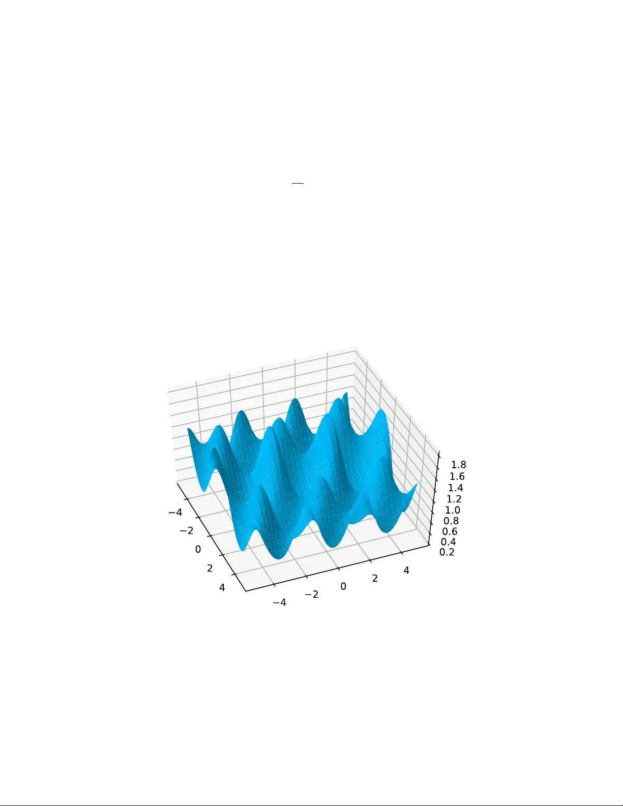
The solutions to the Kadomtsev-Petviashvili equation that arise from a fixed complex algebraic curve are parametrized by a threefold in a weighted projective space, which we name after Boris Dubrovin. Current methods from nonlinear algebra are applie…
Authors: Daniele Agostini, Türkü Özlüm Çelik, Bernd Sturmfels
The Dubro vin threefold of an algebraic curv e Daniele Agostini, T ¨ urk ¨ u ¨ Ozl ¨ um C ¸ elik, and Bernd Sturmfels Abstract The solutions to the Kadom tsev-P etviash vili equation that arise from a fixed complex algebraic curv e are parametrized by a threefold in a weigh ted pro jectiv e space, whic h w e name after Boris Dubro vin. Curren t metho ds from nonlinear algebra are applied to study parametrizations and defining ideals of Dubro vin threefolds. W e highlight the dic hotom y b et w een transcendental representations and exact algebraic computations. Our main result on the algebraic side is a toric degeneration of the Dubrovin threefold in to the pro duct of the underlying canonical curve and a w eigh ted pro jectiv e plane. 1 In tro duction Let C b e a complex algebraic curve of gen us g . The asso ciated Dubr ovin thr e efold D C liv es in a weigh ted pro jectiv e space WP 3 g − 1 , where the w eigh ts are 1, 2 and 3, and each o ccurs precisely g times. The homogeneous coordinate ring of WP 3 g − 1 is the graded polynomial ring C [ U, V , W ] = C [ u 1 , u 2 , . . . , u g , v 1 , v 2 , . . . , v g , w 1 , w 2 , . . . , w g ] , (1) where deg ( u i ) = 1, deg( v i ) = 2 and deg( w i ) = 3, for i = 1 , 2 , . . . , g . P oin ts ( U, V , W ) in the Dubro vin threefold D C corresp ond to solutions of a nonlinear partial differen tial equation that describ es the motion of water w av es, namely the Kadomtsev-Petviashvili (KP) e quation ∂ ∂ x (4 u t − 6 uu x − u xxx ) = 3 u y y . (2) This differential equation represents a universal in tegrable system in tw o spatial dimensions, with co ordinates x and y . The unkno wn function u = u ( x, y , t ) describ es the ev olution in time t of long w a v es of small amplitude with slo w dep endence on the transv erse co ordinate y . The Dubrovin threefold is an ob ject that app ears tacitly in the prominent article [10] on the connection b etw een integrable systems and Riemann surfaces. Another source that men tions this threefold is a man uscript on the Schottky problem b y John Little [22, § 2]. Our aim here is to dev elop this sub ject from the current p erspective of nonlinear algebra [24]. In the algebro-geometric approach to the KP equation (2) one seeks solutions of the form u ( x, y , t ) = 2 ∂ 2 ∂ x 2 log τ ( x, y , t ) + c, (3) 1 where c ∈ C is a constant. The function τ = τ ( x, y , t ) is kno wn as the τ -function in the theory of integrable systems. A sufficient condition for (2) to hold is the quadratic PDE ( τ xxxx τ − 4 τ xxx τ x +3 τ 2 xx ) + 4( τ x τ t − ττ xt ) + 6 c ( τ xx τ − τ 2 x ) + 3( ττ y y − τ 2 y ) + 8 d τ 2 = 0 . (4) This is kno wn as Hir ota’s biline ar form . The scalars c, d ∈ C are uniquely determined b y τ . One constructs τ -functions from an algebraic curv e C of genus g using the metho d de- scrib ed in [10, 11]. Let B b e a Riemann matrix for C . This is a symmetric g × g matrix with en tries in C whose real part is negativ e definite. Its construction from C is shown in (24). F ollo wing [10, equation (1.1.1)], w e in tro duce the asso ciated Riemann theta function θ = θ ( z | B ) = X u ∈ Z g exp 1 2 u T B u + u T z . (5) The vector of unkno wns z = ( z 1 , z 2 , . . . , z g ) is now replaced by a linear com bination of the v ectors U, V , W , seen ab o v e in our p olynomial ring (1). The result is the sp ecial τ -function τ ( x, y , t ) = θ ( U x + V y + W t + D | B ) , (6) where D ∈ C g is also a parameter. The Dubr ovin thr e efold D C comprises triples ( U, V , W ) for whic h the follo wing condition holds: there exist c, d ∈ C such that, for all v ectors D ∈ C g , the function (6) satisfies the equation (4). This implies that (3) satisfies (2). A celebrated result due to Igor Kric hev er [10, Theorem 3.1.3] states that such solutions exist and can b e constructed from every smo oth p oint on the curv e C . This ensures that D C is a threefold. Kric hev er’s construction of solutions to the KP equation amounts to a parametrization of the Dubro vin threefold D C b y abelian functions. This transcenden tal parametrization will b e review ed in Section 2. In Section 3 we present an alternativ e parametrization, v alid after a linear c hange of co ordinates in WP 3 g − 1 , that is entirely algebraic. In particular, we shall see that, for curves C defined ov er the rational num b ers Q , the Dubro vin threefold D C is also defined ov er Q . W e now present a running example whic h illustrates this p oin t. Example 1.1. Let C b e the genus 2 curve defined by y 2 = x 6 − 1. Its Dubro vin threefold D C liv es in WP 5 . By the construction in Section 3, it has the algebraic parametrization u 1 = aU 1 , u 2 = aU 2 , v 1 = a 2 V 1 + 2 bU 1 , v 2 = a 2 V 2 + 2 bU 2 , w 1 = a 3 W 1 + 3 abV 1 + cU 1 , w 2 = a 3 W 2 + 3 abV 2 + cU 2 , (7) where a, b, c and x are free parameters, we sp ecify y = √ x 6 − 1, and we abbreviate U 1 = − 1 y , U 2 = − x y , V 1 = 3 x 5 y 3 , V 2 = 2 y 2 +3 y 3 , W 1 = − (12 y 2 +27) x 4 2 y 5 , W 2 = − (6 y 2 +27) x 5 2 y 5 . (8) Ev ery p oin t ( U, V , W ) on the threefold D C giv es rise to a τ -function (6) that satisfies (4). Using standard implicitization metho ds [24, § 4.2], we compute the homogeneous prime ideal of the Dubrovin threefold D C . This ideal is minimally generated b y the fiv e p olynomials 3 u 5 1 + 2 u 2 2 w 1 − 2 u 1 u 2 w 2 + 3 u 1 v 2 2 − 3 u 2 v 1 v 2 , 3 u 5 2 − 2 u 2 1 w 2 + 2 u 1 u 2 w 1 − 3 u 2 v 2 1 + 3 u 1 v 1 v 2 , 9( u 4 1 u 4 2 − u 4 1 v 2 1 + u 4 2 v 2 2 ) − 4( u 2 w 1 − u 1 w 2 ) 2 , 9( u 3 1 u 4 2 v 1 − u 3 1 v 3 1 + u 4 1 u 3 2 v 2 + u 3 2 v 3 2 ) + 6( u 4 1 v 1 w 1 − u 4 2 v 2 w 2 ) − 4( u 2 w 1 − u 1 w 2 )( v 2 w 1 − v 1 w 2 ) , 9( u 2 1 u 4 2 v 2 1 − u 2 1 v 4 1 + u 3 1 u 3 2 v 1 v 2 + u 4 1 u 2 2 v 2 2 + u 2 2 v 4 2 ) − 4( u 4 1 w 2 1 − u 4 2 w 2 2 ) − 6( u 3 1 u 4 2 w 1 − 2 u 3 1 v 2 1 w 1 + u 4 1 u 3 2 w 2 + 2 u 3 2 v 2 2 w 2 ) − 4( v 2 w 1 − v 1 w 2 ) 2 . (9) These equations are homogeneous of degrees 5 , 5 , 8 , 9 , 10, and their co efficien ts are integers. 2 Theorem 3.7 extends the computation in (9) to arbitrary curves of gen us t w o. W e pass to genus three in Theorem 3.8, by computing the prime ideal of D C for plane quartics C . One can also find p olynomials that v anish on D C directly from the PDE ab ov e. Namely , if w e plug the τ -function (6) in to (4), and w e require the result to b e iden tically zero, then w e obtain p olynomials in U, V , W and c, d whose co efficien ts are expressions in theta constants. Suc h equations w ere derived in [10, § 4.3]. This approach will b e studied in Section 4, where w e fo cus on the numerical ev aluation of theta constants. F or this we use the pack age in [3]. In Section 5 w e mo ve on to curv es C of arbitrary genus. Theorem 5.3 iden tifies an explicit initial ideal for the Dubro vin threefold D C . Geometrically , this is a toric degeneration of D C in to the pro duct of the canonical mo del of C with a w eigh ted pro jective plane WP 2 . F or gen us four and higher, w e run into the Schottky problem: most Riemann matrices B do not arise from algebraic curv es. A solution using the KP equation w as given by Shiota [20, 26]. His characterization of v alid matrices B amounts to the existence of the Dubrovin threefold. In Sec tion 6 we examine sp ecial Dubrovin threefolds, arising from curv es that are singular and reducible. W e fo cus on tropical degenerations, where the theta function turns into a finite exp onen tial sum, and no de-free degenerations, where the theta function turns in to a p olynomial [12]. These were studied for gen us three in the con text of theta surfaces [4, § 5]. 2 P arametrization b y Ab elian F unctions A parametric represen tation of the Dubro vin threefold D C is given in [10, equation (3.1.24)]. This follows Kric hev er’s result on the algebro-geometric construction of solutions to the KP equation. One obtains expressions for the co ordinates of U, V , W by in tegrating normalized differen tials of the second kind on the curv e C . In this section we develop this in detail. W e fix a symplectic basis a 1 , b 1 , . . . , a g , b g for the first homology group H 1 ( C, Z ) of a compact Riemann surface C of gen us g . F or an y p oin t p ∈ C , w e choose three normal- ized differentials of the second type, denoted Ω (1) , Ω (2) and Ω (3) . These are meromorphic differen tials on C , with p oles only at p , and with lo cal expansions at p of the form Ω (1) = − 1 z 2 dz + . . . , Ω (2) = − 2 z 3 dz + . . . , Ω (3) = − 3 z 4 dz + · · · . (10) Here z is a lo cal co ordinate and the dots denote the regular terms. By [10, equation (3.1.24)], w e compute the co ordinates of the vectors U, V , W by integrating these differential forms: u i = Z b i Ω (1) , v i = Z b i Ω (2) , w i = Z b i Ω (3) for i = 1 , 2 , . . . , g . (11) These in tegrals can b e ev aluated using a suitable basis for the holomorphic differentials on C . Namely , supp ose that ω 1 , ω 2 , . . . , ω g is a basis of holomorphic differentials such that Z a j ω k = 2 π i · δ j k , (12) where i = √ − 1 and we use the Kroneck er δ notation. F or such a sp ecial basis, we can compute a symmetric Riemann matrix B = ( B j k ) for the curve C by the following in tegrals: 3 B j k = Z b j ω k for 1 ≤ j, k ≤ g . Around the p oint p on C , we can write eac h holomorphic differential in our basis as ω k = H k ( z ) dz , (13) where H k ( z ) is a holomorphic function of the lo cal co ordinate z . W e denote the first and second deriv ativ e of this function by ˙ H k ( z ) and ¨ H k ( z ). Our differen tials of the second type are Ω (1) = − ω (1) , Ω (2) = − 2 ω (2) , Ω (3) = − 3 ω (3) , (14) where ω ( n ) has a lo cal expansion ω ( n ) = 1 z n +1 dz + . . . . No w, [10, Lemma 2.1.2] sho ws that Z b j ω (1) = H j ( p ) , Z b j ω (2) = 1 2 ˙ H j ( p ) , Z b j ω (3) = 1 6 ¨ H j ( p ) . (15) Putting all of this together, we record the follo wing result: Prop osition 2.1. L et p b e a smo oth p oint on the genus g curve C . The ve ctors in (11) ar e U = − H 1 ( p ) . . . H g ( p ) , V = − ˙ H 1 ( p ) . . . ˙ H g ( p ) , W = − 1 2 ¨ H 1 ( p ) . . . ¨ H g ( p ) . (16) These formulas sp e cify a τ -function (6) , with an arbitr ary ve ctor D ∈ C g , such that the func- tion u ( x, y , t ) define d in (3) is a solution to the KP e quation (2) for some c onstant c ∈ C . Pr o of. W e substitute (14) into (11), and we then use (15) to obtain the form ulas (16). The second assertion is Kric hev er’s result [10, Theorem 3.1.3] mentioned in the Introduction. Prop osition 2.1 expresses ( U, V , W ) as a function of the p oin t p on the curve C . This defines a map from C into the weigh ted pro jective space whose co ordinate ring equals (1): C → WP 3 g − 1 , p 7→ ( U, V , W ) = − H 1 , . . . , H g , ˙ H 1 , . . . , ˙ H g , 1 2 ¨ H 1 , . . . , 1 2 ¨ H g . (17) The image curve is a lifting of the canonical mo del from P g − 1 whic h w e call the lifte d c anonic al curve . Indeed, if we consider only the U -co ordinates in (16) then these define the canonical map from C into P g − 1 . This is an embedding if C is not h yp erelliptic. F or h yp erelliptic curv es of genus g ≥ 2, the canonical map is a 2-to-1 cov er of the rational normal curve. Our construction of lifting the canonical curve from P g − 1 to WP 3 g − 1 is not intrinsic. The map specified in (11) or (16) dep ends on the c hoice of a local co ordinate z around p . Supp ose w e apply an analytic change of lo cal co ordinates, ˜ z = φ ( z ), around p on C . Then our basis of holomorphic differentials can b e expressed, using some holomorphic functions G i , as ω i = G i ( ˜ z ) d ˜ z = G i ( φ ( z )) φ 0 ( z ) dz = H i ( z ) dz for i = 1 , 2 , . . . , g . (18) 4 Using the chain rule from calculus, we find H i ( p ) ˙ H i ( p ) ¨ H i ( p ) = φ 0 (0) 0 0 φ 00 (0) φ 0 (0) 2 0 φ 000 (0) 3 φ 00 (0) φ 0 (0) φ 0 (0) 3 G i ( p ) ˙ G i ( p ) ¨ G i ( p ) . (19) Setting a = φ 0 (0) , b = φ 00 (0) / 2 and c = φ 000 (0) / 2, we consider the matrix group G = a 0 0 2 b a 2 0 c 3 ab a 3 a ∈ C ∗ , b, c ∈ C ⊂ GL(3 , C ) . (20) The group G acts on the weigh ted pro jective space WP 3 g − 1 as follows: a 0 0 2 b a 2 0 c 3 ab a 3 · u i v i w i = au i 2 bu i + a 2 v i cu i + 3 abv i + a 3 w i for i = 1 , 2 , . . . , g . (21) The orbit of a giv en p oin t ( e U , e V , f W ) on D C under the action is the surface defined b y ˜ u i u j − ˜ u j u i , ˜ u i ( ˜ u j v i − ˜ u i v j ) − u i ( ˜ v i u j − ˜ v j u i ) , and 2 ˜ u 2 j ( ˜ u j w i − ˜ u i w j ) − 2 u 2 j ( ˜ w i u j − ˜ w j u i ) + 3 ˜ u j u j ( ˜ v j v i − ˜ v i v j ) for 1 ≤ i < j ≤ g . (22) In these equations, the quantities u i , v i , w i are v ariables while ˜ u i , ˜ v i , ˜ w i are complex n um b ers. This surface defined by (22) is isomorphic to the weigh ted pro jectiv e plane WP 2 = P (1 , 2 , 3). The Dubrovin threefold D C is the union of a 1-parameter family of suc h surfaces in WP 3 g − 1 . Namely , the union is tak en o ver all points ( e U , e V , f W ) in the image of the map (17). In Theorem 5.3 we shall presen t a toric degeneration that turns this family in to a pro duct. Remark 2.2. W e here regard D C as an irreducible v ariety . This is sligh tly inconsisten t with the Introduction, where D C w as defined in terms of solutions to the KP equation. The reason is the in v olution ( U, V , W ) 7→ ( U, − V , W ) on WP 3 g − 1 . By [10, (4.2.5)], this inv olution preserv es the prop ert y that (6) solves (4), and it sw aps D C with an isomorphic copy D − C . Th us the parameter space for solutions (3) to (2) would b e the reducible threefold D C ∪ D − C . In our parametric represen tation of the Dubrovin threefold D C , w e required holomorphic differen tials (13) that are adapted to a symplectic homology basis in the sense of (12). This h yp othesis is essential when w e seek solutions to the KP equation. Ho w ever, it is not needed when studying algebraic or geometric prop erties of D C . F or that we allow a linear change of co ordinates. This is imp ortan t in practice b ecause differentials ω k that satisfy (12) may not b e readily a v ailable. W e shall see this in the symbolic computations in Section 3. In what follo ws w e explain how to w ork with an arbitrary basis of holomorphic differentials (13). Let e ω 1 , . . . , e ω g b e suc h a basis. W e consider the corresp onding g × g p erio d matrices Π a = Z a j e ω i ! ij and Π b = Z b j e ω i ! ij . (23) 5 F rom these t w o non-symmetric matrices, we obtain the symmetric Riemann matrix B = 2 π i · Π − 1 a Π b . (24) F or a giv en plane curve C , the matrices (23) and (24) can b e computed using numerical metho ds. In our exp erimen ts, w e used the SageMath implemen tation due to Bruin et al. [8]. Giv en this data, a normalized basis of differen tials as in (12) is obtained as follows: ( ω 1 , ω 2 , . . . , ω g ) T = 2 π i · Π − 1 a ( e ω 1 , e ω 2 , . . . , e ω g ) T . (25) The linear transformation in (25) induces a linear c hange of coordinates on the Dubrovin threefold D C in WP 3 g − 1 as follows. Consider a smo oth p oint p ∈ C and a lo cal co ordinate z around p . W e write e ω i = e H i ( z ) dz , where e H i is holomorphic, and w e define v ectors as in (16): e U := − e H 1 ( p ) . . . e H g ( p ) , e V := − ˙ e H 1 ( p ) . . . ˙ e H g ( p ) , f W := − 1 2 ¨ e H 1 ( p ) . . . ¨ e H g ( p ) . (26) Then the vectors U, V , W for the adapted basis ω 1 , ω 2 , . . . , ω g are given by U = 2 π i · Π − 1 a e U , V = 2 π i · Π − 1 a e V , W = 2 π i · Π − 1 a f W . (27) An y suc h linear change of co ordinates commutes with the action of the group G as in (21). Remark 2.3. In conclusion, for any basis e ω 1 , e ω 2 , . . . , e ω g of holomorphic differentials, w e can define a Dubro vin threefold in WP 3 g − 1 . It is the union of all G -orbits of the p oin ts ( e U , e V , f W ) in (26). An y tw o suc h Dubrovin threefolds are related to eac h other via a linear change of co ordinates. This scenario in WP 3 g − 1 is analogous to that for canonical curv es in P g − 1 . Thus, to compute Dubro vin threefolds and their prime ideals, w e can use an y basis e ω 1 , e ω 2 , . . . , e ω g of our c hoosing. Whenever this is clear, w e omit the e sup erscript from our notation. How ever, if we wan t the Dubro vin threefold to parametrize solutions (3) of the KP equation, then we m ust use a normalized basis as in (12) or p erform the linear c hange of co ordinates in (27). T o illustrate Remark 2.3, we examine KP solutions arising from our running example. Example 2.4. Consider an y zero e U , e V , f W in WP 5 of the five p olynomials in (9). Here, D C w as computed using the basis of differentials e ω 1 , e ω 2 giv en in (36) b elo w. This basis relates to an adjusted basis via p erio d matrices which we computed numerically using SageMath : Π a = 1 . 2143253 i 1 . 0516366 + 0 . 6071627 i − 1 . 2143253 − 0 . 6071627 − 1 . 0516366 i , Π b = − 1 . 0516366 − 0 . 6071627 i 1 . 2143253 i − 0 . 6071627 − 1 . 0516366 i 1 . 2143253 . W e can no w use these matrices to construct t wo-phase solutions of the KP equation (2). First w e compute the follo wing Riemann matrix for the curve C = { y 2 = x 6 − 1 } in Example 1.1: B = 2 π i · Π − 1 a Π b = − 7 . 25519746 3 . 62759872 3 . 62759872 − 7 . 25519746 = 2 π √ 3 2 1 1 2 . 6 This allows us to ev aluate the theta function θ ( z | B ), e.g. using the Julia pack age de- scrib ed in [3]. The ev aluation is done, for an y fixed D ∈ C 2 , at the points U x + V y + W z + D , where the co efficients U = ( u 1 , u 2 ) T , V = ( v 1 , v 2 ) T and W = ( w 1 , w 2 ) T are obtained from e U , e V , f W b y the linear c hange of co ordinates in (27). The resulting function u ( x, y , t ) in (3) solv es (2) for an appropriate constant c . In this manner, the Dubrovin threefold D C that is giv en by (9) represents a 3-parameter family of tw o-phase solutions to the KP equation (2). F or a n umerical example, fix p = (2 , √ 63) on C . The corresp onding parameters are U = 0 . 133702 + 0 . 111777 i − 0 . 059901 − 0 . 119802 i , V = − 0 . 151861 − 0 . 140376 i 0 . 091278 + 0 . 122654 i , W = 0 . 131964 + 0 . 13077 i − 0 . 094538 − 0 . 09780 i . W e use the pro cedure in Remark 4.5 b elo w to estimate the constan ts c and d as follows: c = 0 . 02546003 + 0 . 15991389 i and d = 0 . 00437723 + 0 . 00078777 i. (28) The corresp onding solution u ( x, y , t ) is complex-v alued and it has singularities. W e close this section with an example where the KP solution is real-v alued and regular. Figure 1: A w a v e at time t = 0 deriv ed from the T rott curv e. Example 2.5. A prominen t instance of a plane quartic C is the T r ott curve f ( x, y ) = 144( x 4 + y 4 ) − 225( x 2 + y 2 ) + 350 x 2 y 2 + 81 . (29) This curve is smo oth. Its real picture consists of four ov als [4, Figure 7]. W e fix a symplectic basis of paths where the a i are purely imaginary and the b j are real. In particular, the 7 paths b j corresp ond to ov als of C . Using this basis, together with the basis of holomorphic differen tials in Example 3.5, w e compute the p erio d matrices and the Riemann matrix: Π a = 0 . 01384015942 0 . 02768031884 0 . 01384015942 0 . 01384015941 0 − 0 . 01384015941 0 . 02348847438 0 0 . 02348847438 i , B = − 2 π 1 . 57412534343470 − 0 . 671587878369476 − 0 . 230949586695748 − 0 . 671587878369476 1 . 57412534206005 − 0 . 671587878369476 − 0 . 230949586695747 − 0 . 671587878369476 1 . 57412534343470 . W e fix the p oint (0 , 1) on C , and we compute an asso ciated p oin t on the Dubrovin threefold: 0 , − 1 126 , − 1 126 , − 1 126 , 0 , 0 , 0 , − 1550 55566 , − 1325 37044 ∈ D C ⊂ WP 8 . (30) The corresp onding KP solution u ( x, y , t ) is real-v alued and has no singularities. The graph of the function R 2 → R , ( x, y ) 7→ u ( x, y , 0), up to a translation, is sho wn in Figure 1. Equations that define D C are giv en to wards the end of Example 3.5. Every p oin t ( U, V , W ) with U 6 = 0 that satisfies (35) gives rise to a KP solution lik e Figure 1. Note that the homo- genenized T rott quartic f u 1 /u 3 , u 2 /u 3 u 4 3 is a linear combination of the three polynomials in (35). F or an analytic p ersp ectiv e on the defining ideal of the threefold D C see Example 4.8. 3 Algebraic Implicitization for Plane Curv es This section is concerned with algebraic represen tations of Dubro vin threefolds. The parametrization describ ed in Section 2 will b e made explicit for plane curves, in a form that is suitable for symbolic computations. This sets the stage for implicitization [24, § 4.2]. In Theorems 3.7 and 3.8 w e determine the prime ideals of all implicit equations for gen us tw o and three resp ectively . The connection to the KP equation requires a basis change for the holomorphic differen tials, as explained in Remark 2.3. Our v arieties giv e rise to KP solutions after that basis change. Bearing this in mind, w e can now safely omit the e sup erscripts. Let C b e a compact Riemann surface, represented by a p ossibly singular curv e C o in the complex affine plane C 2 . The curve C o is defined by an irreducible p olynomial f ( x, y ). W e assume that f lies in Q [ x, y ], i.e. all co efficients of f are rational n um b ers. This ensures that the computations in this section can b e carried out sym b olically ov er Q . Our first goal is to start from f and find a parametric representation of the Dubrovin threefold D C in WP 3 g − 1 . Let d = degree( f ) and g = genus( C ) ≤ d − 1 2 . W e assume throughout that y d app ears with nonzero co efficien t in f . The partial deriv atives of f are denoted b y f x = ∂ f /∂ x and f y = ∂ f /∂ y . Similarly , w e write f xx , f xy , f y y , f xxx , . . . for higher-order deriv ativ es. W e often view the y -co ordinate on C o as a (multi-v alued) function of x . It is then denoted y ( x ). As in [8, § 3.1], w e c ho ose p olynomials h 1 , h 2 , . . . , h g ∈ Q [ x, y ] such that the follo wing set of holomorphic differentials is a basis for the complex vector space H 0 ( C, Ω 1 C ): n ω i = H i ( x, y ) dx i = 1 , 2 , . . . , g o where H i = h i ( x, y ) f y ( x, y ) . (31) 8 Example 3.1. Let f b e a general p olynomial of degree d in Q [ x, y ]. The curv e C o is smooth, w e hav e g = d − 1 2 , and our Riemann surface C is the closure of C o in P 2 . F or the numerator p olynomials h 1 , . . . , h g w e tak e the monomials of degree at most d − 3. Thus, (31) b ecomes x i y j f y dx 0 ≤ i + j ≤ d − 3 . (32) W orking mo dulo the principal ideal h f i , we regard y = y ( x ) as an algebraic function in x . W e no w record the following imp ortant consequence of Prop osition 2.1. Corollary 3.2. The formulas for the c olumn ve ctors U, V , W in (16) , c omp ose d with the gr oup action in (21) , give an algebr aic p ar ametrization of the Dubr ovin thr e efold D C . This p ar ametrization has c o or dinates in K [ a, b, c ] , wher e K is the field of fr actions of Q [ x, y ] / h f i . Pr o of. The functions H i in the differentials ω i are rational in x and y , so they define elements in the function field K of the curve C . W e write y = y ( x ), so x is our lo cal parameter on C . W e use dot notation for deriv ativ es with resp ect to x . By implicit differentiation, we find ˙ y = − f x f y and ¨ y = − f 2 x f y y − 2 f y f x f xy + f 2 y f xx f 3 y . (33) W e similarly tak e deriv atives of H i = H i ( x, y ( x )) with respect to x . This yields rational form ulas for the co ordinates H i , ˙ H i , ¨ H i of U, V , W . Again, we view these as elemen ts in K . Example 3.3 (Smo oth plane curv es) . Let C b e a smo oth plane curve of degree d describ ed b y an affine equation f ( x, y ) = 0. F or the basis of holomorphic differentials w e take (32), but with negative signs. The g co ordinates of the canonical curv e are elements in K : U = ( u 1 , u 2 , . . . , u g ) = − 1 f y 1 , x, y , x 2 , xy , . . . , y d − 3 . The first co ordinates of V and W are deriv ed from those of U by implicit differentiation: v 1 = ˙ u 1 = f y f xy − f x f y y f 3 y , w 1 = ¨ u 1 2 = − 3 f 2 x f 2 y y + f 2 x f y f y yy + 6 f x f y f xy f y y − 2 f x f 2 y f xy y − 2 f 2 y f 2 xy − f 2 y f xx f y y + f 3 y f xxy 2 f 5 y . The other co ordinates of V and W can be computed b y applying the pro duct rule and implicit differentiation to the form ula u k = x i y j · u 1 . W e thus derive the formulas v k = ˙ u k = ˙ u 1 x i y j + u 1 x i − 1 y j − 1 ( iy + j x ˙ y ) = ( f y f xy − f x f y y ) x i y j − if 2 y x i − 1 y j + j f x f y x i y j − 1 f 3 y . w k = ¨ u k 2 = ¨ u 1 2 x i y j + ˙ u 1 ( ix i − 1 y j + j x i y j − 1 ˙ y ) + u 1 2 i ( i − 1) x i − 2 y j + 2 ij x i − 1 y j − 1 ˙ y + j ( j − 1) x i y j − 2 ˙ y 2 + j x i y j − 1 ¨ y . All of these expressions are rational functions in x and y with co efficien ts in Q . W e regard them as elements in K , the field of fractions of Q [ x, y ] / h f i . In practice, this means replacing the n umerator p olynomial in Q [ x, y ] and reducing it to a normal form mo dulo the ideal h f i . 9 Remark 3.4. In the parametrization described in Corollary 3.2, w e can choose all co or- dinates to b e p olynomials. Indeed, consider the formulas derived in Example 3.3. W e see that U, V , W ha v e the common denominators f y , f 3 y , f 5 y resp ectiv ely . W e can th us clear all denominators in ( U, V , W ) b y multiplying each co ordinate by an appropriate p o w er of f y , in a manner that do es not change the corresp onding p oin t in WP 3 g − 1 . Thereafter we apply the action of the group G . W e obtain a p olynomial map with the same image D C in WP 3 g − 1 . In our computational exp eriments w e started out with canonical curves of gen us three and with hyperelliptic curves. The following tw o examples illustrate these classes of curves. Example 3.5. Let C be the T rott curve which was studied in Example 2.5. The following three differen tial forms constitute our basis for the space H 0 ( C, Ω 1 C ) w e c hose in Example 3.1: ω 1 = 1 f y dx, ω 2 = x f y dx, ω 3 = y f y dx. (34) Note that u 1 = − 1 /f y , u 2 = − x/f y and u 3 = − y /f y , where f y = 700 x 2 y + 576 y 3 − 450 y . By reducing the formulas for the V - and W -co ordinates in Example 3.3 mo dulo f , we obtain: v 1 = 12(39556 x 3 y 2 − 4650 x 3 − 13950 y 2 + 2025 x ) f − 3 y , v 3 = 496(638 x 2 − 225) xf − 3 y , v 2 = 4(79112 x 4 y 2 − 13950 x 4 − 13950 x 2 y 2 + 6075 x 2 − 3969 y 2 ) f − 3 y , w 1 = 1 3 (450627015168 x 10 + 1095273995200 x 8 y 2 − 982215036000 x 8 − 1260877167000 x 6 y 2 +710159081508 x 6 + 430938071100 x 4 y 2 − 196724295000 x 4 − 30435203250 x 2 y 2 +11445723549 x 2 − 5650169175 y 2 + 2242385775) f − 5 y , w 2 = 1 3 (225313507584 x 11 + 547636997600 x 9 y 2 − 391782402000 x 9 − 355914999000 x 7 y 2 +132297850476 x 7 − 102485711700 x 5 y 2 + 68233160700 x 5 + 101045778750 x 3 y 2 − 45254399085 x 3 − 16950507525 y 2 + 6727157325) f − 5 y , w 3 = 62 3 (25236728 x 6 − 14833500 x 4 +1652778 x 2 +297675)(144 x 4 +350 x 2 y 2 − 225 x 2 − 225 y 2 +81) y f − 5 y . T o set up our implicitization problem, we first replace the ab ov e form ulas for U, V , W b y f 2 y U, f 4 y V , f 6 y W in order to get rid of the denominators. Then, applying the group action (21), w e write the co ordinates on D C as af 2 y U, 2 bf 2 y U + a 2 f 4 y V , cf 2 y U + 3 abf 4 y V + a 3 f 6 y W . These are nine p olynomials in fiv e unkno wns a, b, c, x, y . Regarded mo dulo the equation f ( x, y ) = 0, this is the parametrization of the Dubro vin threefold D C that is promised in Remark 3.4. The nine expressions are quite complicated. But they satisfy the follo wing six nice relations: 450 u 2 1 u 3 + 450 u 2 2 u 3 − 324 u 3 3 + u 2 v 1 − u 1 v 2 , 700 u 2 1 u 2 + 576 u 3 2 − 450 u 2 u 2 3 + u 3 v 1 − u 1 v 3 , 576 u 3 1 + 700 u 1 u 2 2 − 450 u 1 u 2 3 − u 3 v 2 + u 2 v 3 , 450 u 1 u 3 v 1 + 450 u 2 u 3 v 2 + 225 u 2 1 v 3 + 225 u 2 2 v 3 − 486 u 2 3 v 3 + u 2 w 1 − u 1 w 2 , 700 u 1 u 2 v 1 + 350 u 2 1 v 2 + 864 u 2 2 v 2 − 225 u 2 3 v 2 − 450 u 2 u 3 v 3 + u 3 w 1 − u 1 w 3 , 864 u 2 1 v 1 + 350 u 2 2 v 1 − 225 u 2 3 v 1 + 700 u 1 u 2 v 2 − 450 u 1 u 3 v 3 − u 3 w 2 + u 2 w 3 . (35) These are the six relations in (39) and (40). After saturation, as explained in Theorem 3.8, these generate the prime ideal of D C . All computations are done using Gr¨ obner bases o ver Q . W e illustrate the situation for h yp erelliptic curves in the most basic case of genus tw o. 10 Example 3.6. Let C b e a general curv e of genus tw o. It is defined by an equation y 2 = F ( x ) , where F ( x ) = ( x − a 1 )( x − a 2 ) · · · ( x − a 6 ) with a i ∈ C . A basis for the space of differential forms on the hyperelliptic curve C consists of ω 1 = 1 √ F dx and ω 2 = x √ F dx. (36) W e tak e the first and second x -deriv ative of their co efficien ts. According to the form ulas of (16), the resulting formula for the p oint ( U, V , W ) = ( u 1 , u 2 , v 1 , v 2 , w 1 , w 2 ) in WP 5 equals − 1 √ F , − x √ F , F 0 2 F √ F , xF 0 − 2 F 2 F √ F , 2 F F 00 − 3( F 0 ) 2 8 F 2 √ F , 2 xF F 00 + 4 F F 0 − 3 x ( F 0 ) 2 8 F 2 √ F . (37) This provides the algebraic parametrization in Corollary 3.2. In particular, if w e go back to Example 1.1, then the parametrization in (37) b ecomes the one presented in equation (8). W e conclude this section with t wo general theorems on the prime ideals defining D C . The first one, Theorem 3.7, explains the relations we saw in (9). Here we work in the p olynomial ring C [ u 1 , u 2 , v 1 , v 2 , w 1 , w 2 ] with the grading deg ( u 1 ) = deg ( u 2 ) = 1, deg ( v 1 ) = deg ( v 2 ) = 2, and deg ( w 1 ) = deg( w 2 ) = 3. The group G acts on this ring via (21). The follo wing tw o p olynomials of degree five are in v ariant (up to scaling by a 5 ) under this G -action: I 1 = 2 u 2 2 w 1 − 2 u 1 u 2 w 2 + 3 u 1 v 2 2 − 3 u 2 v 1 v 2 , I 2 = 2 u 2 1 w 2 − 2 u 1 u 2 w 1 + 3 u 2 v 2 1 − 3 u 1 v 1 v 2 . The tuple (37) parametrizes an algebraic curve in C 6 . The orbit of this curve under the group G is a 4-dimensional v ariety in C 6 . Its image in WP 5 is the Dubro vin threefold D C . W e write ¯ F ( u 1 , u 2 ) = F ( u 2 /u 1 ) u 6 1 for the binary sextic obtained by homogenizing F ( x ). Theorem 3.7. L et C b e a genus two curve, r epr esente d by a sextic F ( x ) as in Example 3.6. Ther e ar e two line arly indep endent quintics that vanish on the Dubr ovin thr e efold D C : ∂ ¯ F /∂ u 1 − 2 I 1 and ∂ ¯ F /∂ u 2 − 2 I 2 . (38) The prime ide al of the Dubr ovin thr e efold is minimal ly gener ate d by five p olynomials, of de gr e es 5 , 5 , 8 , 9 , 10 . This ide al is obtaine d fr om that gener ate d by (38) via satur ating h u 1 , u 2 i . Pr o of. This is verified by a computer algebra ov er the field L = Q ( a 1 , a 2 , . . . , a 6 ). The co- ordinates of the parametrization (37) live in L [ x, y ] / h y 2 − F ( x ) i , and we chec k that (38) v anishes when we substitute (37) for ( U, V , W ). The tw o equations in (38) define a v ariet y of co dimension tw o in WP 5 . The irreducible threefold D C m ust b e one of its irreducible com- p onen ts. W e saturate (38) b y h u 1 , u 2 i , thus removing an extraneous nonreduced comp onen t on { U = 0 } . The result of this saturation is an ideal with five minimal generators of degrees 5 , 5 , 8 , 9 , 10. A further computation in Macaulay2 verifies that this ideal is prime. This implies that the irreducible threefold defined by this prime ideal must b e equal to D C . 11 W e next turn to genus three. Assuming that C is non-h yp erelliptic, its canonical mo del is a quartic in P 2 with co ordinates U = ( u 1 , u 2 , u 3 ). W e seek the prime ideal of the Dubrovin threefold D C in WP 8 . This ideal lives in the p olynomial ring C [ U, V , W ] in nine v ariables. Here C can b e replaced by the subfield ov er which C is defined. F or us, this is usually Q . The next theorem explains the relations in (35). It should b e compared with Lemma 5.7. Theorem 3.8. L et C b e a smo oth algebr aic curve of genus thr e e given by a ternary quartic f ( u 1 , u 2 , u 3 ) . The prime ide al of its Dubr ovin thr e efold is minimal ly gener ate d by 17 p olyno- mials in C [ U, V , W ] . These have de gr e es 3 , 3 , 3 , 4 , 4 , 4 , 5 , 5 , 5 , 8 , 8 , 9 , 9 , 10 , 10 , 11 , 12 . The first six gener ators suffic e up to satur ation by h u 1 , u 2 , u 3 i . The thr e e cubic ide al gener ators ar e ∂ f ∂ u 1 + u 2 v 2 u 3 v 3 , ∂ f ∂ u 2 − u 1 v 1 u 3 v 3 , ∂ f ∂ u 3 + u 1 v 1 u 2 v 2 . (39) Fixing the quintic g = v 1 · ∂ f /∂ u 1 + v 2 · ∂ f /∂ u 2 + v 3 · ∂ f /∂ u 3 , the thr e e quartic gener ators ar e ∂ g ∂ u 1 + 2 u 2 w 2 u 3 w 3 , ∂ g ∂ u 2 − 2 u 1 w 1 u 3 w 3 , ∂ g ∂ u 3 + 2 u 1 w 1 u 2 w 2 . (40) The cubics (39) imply that the quartic f ( u 1 , u 2 , u 3 ) is in the ideal. This is consisten t with the general theory (cf. [10, § 4.3]) since the quartic { f = 0 } in P 2 is a canonical curve. Pr o of. Equations (39) and (40) can b e prov ed by a direct computation for a general quartic with indeterminate co efficien ts. That symbolic computation is facilitated b y the fact that these equations are inv ariant under the action by PGL(3 , C ) on the v ectors U, V , W and the induced action on quartics in u 1 , u 2 , u 3 . So, it suffices to chec k a six-dimensional family of quartic curv es that represen ts a Zariski dense set of orbits. Alternatively , (39) can be deriv ed geometrically by examining the meaning of the vectors U, V in C 3 . The vector U represen ts a p oin t on the canonical curv e which we iden tify with C itself. T o understand the meaning of V , we examine the parametrization of D C giv en in (16). The plane spanned b y U and V in C 3 corresp onds to the tangen t line to C at the p oint U . By Cramer’s rule, this implies that the gradien t of f at U equals up to a scalar m ultiple the v ector whose three co ordinates are the determinants on the righ t hand side of (39). A computation reveals that this scalar m ultiple equals 1. This explains (39), and then (40) follows from the pro of of Lemma 5.7. The v ariet y defined by our equations in WP 8 is irreducible of dimension three outside the lo cus defined by h u 1 , u 2 , u 3 i . This follo ws immediately from the structure of the equations. First, we hav e an irreducible curve in the P 2 with co ordinates U . F or ev ery p oin t on that curv e, (39) giv es t w o indep endent linear equations in V . After c ho osing U and V , (39) gives t w o indep enden t linear equations in W . Th us there are three degrees of freedom, and our v ariet y is irreducible since the equations ov er C are linear. The precise num b er and degrees of minimal generators for the prime ideal are obtained by computations with generic f . The next section offers an alternativ e n umerical view on implicitizing Dubro vin threefolds. A conceptual explanation of Theorem 3.8, v alid for arbitrary gen us g , app ears in Theorem 5.3. 12 4 T ranscenden tal Implicitization Our workhorse in this section is the Riemann theta function θ ( z | B ), defined by its series expansion in (5). W e c hose the Riemann matrix B as in [10], with negativ e definite real part. This differs by a factor 2 π i from the Riemann matrix in the algebraic geometry literature. The latter is also used in the Julia pack age [3]. This section builds on [10, § IV.2]. W e show ho w theta series lead to p olynomials in C [ U, V , W ] that v anish on the Dubro vin threefold of a curve C of genus g with Riemann matrix B . A p oin t ( U, V , W ) lies in this threefold if and only if the τ -function of (6) satisfies Hirota’s bilinear relation (4) for some c, d ∈ C and any D ∈ C g . In this definition, b y the Dubrovin threefold w e mean the union D C ∪ D − C referred to in Remark 2.2. Hence, the irreducible threefold D C , studied algebraically in Section 3, o ccurs in tw o different sign copies in the v ariety defined here. F or what follows we prefer: Definition 4.1 (Big Dubro vin threefold) . Let WP 3 g +1 b e the weigh ted pro jectiv e space with co ordinates ( U , V , W, c, d ) where the new v ariables c, d ha ve degrees 2 and 4 resp ectiv ely . The big Dubr ovin thr e efold D big C is the set of p oints in WP 3 g +1 suc h that Hirota’s bilinear relation (4) is satisfied for the function τ ( x, y , t ) = θ ( U x + V y + W t + D ), where D ∈ C g is arbitrary . W e b egin by sho wing that the big Dubrovin threefold is indeed an algebraic v ariet y . Giv en an y z in C g , w e write θ ( z ) = θ ( z | B ) for the complex n umber on the righ t in (5). W e set ∂ U := u 1 ∂ ∂ z 1 + · · · + u g ∂ ∂ z g , and w e define ∂ U θ ( z ) to b e the v alue at z of that directional deriv ative of the theta function. This v alue is a linear form in U with complex co efficien ts. W e similarly define ∂ V θ ( z ) and ∂ W θ ( z ). W e also consider the v alues of higher order deriv atives lik e ∂ 4 U θ ( z ) , ∂ 2 V θ ( z ) , ∂ U ∂ W θ ( z ). These are homogeneous p olynomials of degree four in C [ U, V , W ]. F or an y fixed vector z ∈ C g , we define the Hir ota quartic H z to b e the expression ∂ 4 U θ ( z ) · θ ( z ) − 4 ∂ 3 U θ ( z ) · ∂ U θ ( z ) + 3 { ∂ 2 U θ ( z ) } 2 + 4 · ( ∂ U θ ( z ) · ∂ W θ ( z ) − θ ( z ) · ∂ U ∂ W θ ( z )) + 6 c · ∂ 2 U θ ( z ) · θ ( z ) − { ∂ U θ ( z ) } 2 + 3 · θ ( z ) · ∂ 2 V θ ( z ) − { ∂ V θ ( z ) } 2 + 8 d · θ ( z ) 2 . (41) This is a homogeneous quartic in the p olynomial ring C [ U, V , W , c, d ], where c and d hav e degrees 2 and 4 resp ectiv ely . The co efficien ts of the Hirota quartic H z ( U, V , W , c, d ) dep end on the v alues of the theta function θ and its partial deriv ativ es at z . The zero set of H z is in the weigh ted pro jectiv e space WP 3 g +1 . W e consider the in tersection of these hypersurfaces. Prop osition 4.2. The big Dubr ovin thr e efold D big C is the interse ction in WP 3 g +1 of the algebr aic hyp ersurfac es define d by the Hir ota quartics H z , as z runs over al l ve ctors in C g . Pr o of. If we expand the left hand side of Hirota’s bilinear relation (4), then w e obtain the expression H z ( U, V , W , c, d ) for z = U x + V y + W z + D . By definition, a p oin t ( U, V , W , c, d ) ∈ WP 3 g +1 b elongs to D big C if and only if this expression is zero for all x, y , t ∈ C and all D ∈ C g . Since D is arbitrary in C g , the v alue of z = U x + V y + W t + D is also arbitrary . This implies that D big C is the intersection of all the hypersurfaces { H z = 0 } as z ranges ov er C g . F or any z ∈ C g , w e can compute the Hirota quartic H z using n umerical soft w are for ev aluating theta functions and their deriv atives. The state of the art for such softw are is 13 the Julia pac k age in tro duced in [3]. This w as used for the computations rep orted in this section. These differ greatly from the exact sym b olic computations rep orted in Section 3. One drawbac k of Prop osition 4.2 is that the n um ber of Hirota quartics is infinite. W e next deriv e a finite set of equations for D big C via the addition formula for theta functions with c haracteristics. This deriv ation was explained b y Dubro vin in [10, § IV.1]. A half-char acteristic is an element ε ∈ ( Z / 2 Z ) g whic h w e see as a v ector with 0 , 1 entries. Giv en an y tw o half-characteristics ε, δ ∈ ( Z / 2 Z ) g , their theta function with char acteristic is θ ε δ ( z | B ) = X u ∈ Z g exp 1 2 ( u + ε ) T B ( u + ε ) + ( z + 2 π iδ ) T B ( u + ε ) . (42) When ε = δ = 0, this function is precisely the Riemann theta function (5). F or δ = 0 but arbitrary ε , we consider (42) with the doubled p eriod matrix 2 B . This is abbreviated by ˆ θ [ ε ]( z ) := θ ε 0 ( z | 2 B ) . (43) W e are in terested in the v alues ˆ θ [ ε ](0) of these 2 g functions at z = 0. F or fixed B , these are complex num b ers, kno wn as theta c onstants . W e use the term theta constan t also for ev aluations at z = 0 of deriv atives of (43) with the v ector fields ∂ U , ∂ V , ∂ W as ab o v e. With these conv entions, the following expression is a p olynomial of degree four in ( U, V , W , c, d ): F [ ε ] := ∂ 4 U ˆ θ [ ε ](0) − ∂ U ∂ W ˆ θ [ ε ](0) + 3 2 c · ∂ 2 U ˆ θ [ ε ](0) + 3 4 ∂ 2 V ˆ θ [ ε ](0) + d ˆ θ [ ε ](0) . (44) W e call F [ ε ]( U, V , W, c, d ) the Dubr ovin quartic asso ciated with the half-c haracteristic ε . There are 2 g Dubro vin quartics in total, one for eac h half-c haracteristic ε in ( Z / 2 Z ) g . W e find that these quartics can also b e used as implicit equations for the big Dubrovin threefold D big C inside WP 3 g +1 . This follows by combining Prop osition 4.2 with the following result. Prop osition 4.3 (Dubrovin) . The Dubr ovin quartics and the Hir ota quartics sp an the same ve ctor subsp ac e of C [ U, V , W , c, d ] 4 . This sp ac e of quartics defines the big Dubr ovin thr e efold. Pr o of. This result is essentially the one pro ved in [10, Lemma 4.1.1]. A k ey step is the iden tit y H z = 8 · X ε ∈ ( Z / 2 Z ) g ˆ θ [ ε ](2 z ) · F [ ε ] in C [ U, V , W , c, d ] 4 . (45) This is prov ed via the addition formula [10, (4.1.5)], analogously to the deriv ation from (4.1.8) to (4.1.10) in [10]. W e can also inv ert the linear relations in (45) and express the Dubro vin quartics F [ ε ] as C -linear com binations of the Hirota quartics H z . Indeed, the functions z 7→ ˆ θ [ ε ](2 z ) are linearly indep enden t [10, (1.1.11)]. If we tak e z from any fixed set of 2 g general p oin ts in C g then the corresp onding 2 g × 2 g matrix of theta constants ˆ θ [ ε ](2 z ) are in v ertible. The second assertion in Prop osition 4.3 no w follo ws from Prop osition 4.2. Corollary 4.4. The Dubr ovin thr e efold D C is an irr e ducible c omp onent of the image of the big Dubr ovin thr e efold D big C under the map WP 3 g +1 → WP 3 g − 1 , ( U, V , W , c, d ) 7→ ( U, V , W ) . 14 Pr o of. The image of the big Dubro vin threefold D big C in WP 3 g − 1 is also an algebraic threefold. Its equations are obtained from those of D big C b y eliminating the unknowns c and d . In fact, this image is equal to D C ∪ D − C . The second comp onent is explained in Remark 2.2. This follo ws from the characterization of the Dubrovin threefold as a space of KP solutions. Remark 4.5. Consider an y p oin t ( U, V , W ) in the Dubrovin threefold D C ⊂ WP 3 g − 1 . It is given to us numerically . The p oin t has a unique preimage in the big Dubrovin threefold D big C ⊂ WP 3 g +1 . T o compute that preimage, w e plug ( U, V , W ) in to sev eral Hirota quartics H z or Dubrovin quartics F [ ε ]. This results in an o v erdetermined system of linear equations in t w o unknowns c and d . W e use n umerical metho ds to approximately solve these equations. This gives us estimates for c and d . This metho d was used to estimate the constants in (28). Supp ose now that we are given a curve C by w a y of its Riemann matrix B . F or instance, this is the hypothesis for the construction of KP solutions in [11]. W e can compute ap- pro ximations of the quartics H z or F [ ε ] using numerical soft w are for theta functions (cf. [3]). F ollowing [10, § 4.3], w e can then find equations for the canonical mo del of C in P g − 1 . F or an y half-c haracteristic ε ∈ ( Z / 2 Z ) g , we write Q [ ε ] for the Hessian matrix of the function ˆ θ [ ε ]( z ). W e regard Q [ ε ] as a quadratic form in g v ariables. The next lemma characterizes the in ter- section of the subspace of quartics in Prop osition 4.3 with the polynomial subring C [ U, V , W ]. Lemma 4.6. A C -line ar c ombination P λ ε F [ ε ] of the Dubr ovin quartics is indep endent of the two unknowns c and d if and only if it has the form X ε ∈ ( Z / 2 Z ) g λ ε · ∂ 4 U ˆ θ [ ε ] (46) wher e the 2 g c omplex sc alars λ ε satisfy the line ar e quations X ε λ ε · Q [ ε ] = 0 and X ε λ ε · ˆ θ [ ε ] = 0 . (47) The line ar system (47) has maximal r ank, i.e. it has 2 g − g ( g +1) 2 − 1 indep endent solutions ( λ ε ) . Pr o of. Using the quadratic forms Q [ ε ], we can rewrite the Dubro vin quartic (44) as follows: F [ ε ] = ∂ 4 U ˆ θ [ ε ] − Q [ ε ]( U, W ) + 3 2 c Q [ ε ]( U, U ) + 3 4 Q [ ε ]( V , V ) + d ˆ θ [ ε ] . (48) The linear combinations of the F [ ε ] where the v ariables c, d do not app ear ha v e the form X ε λ ε ∂ 4 U ˆ θ [ ε ] − X ε λ ε Q [ ε ]( U, W ) + 3 2 c · X ε λ ε Q [ ε ]( U, U ) + 3 4 X ε λ ε Q [ ε ]( V , V ) + d X ε λ ε ˆ θ [ ε ] , where P ε λ ε ˆ θ [ ε ] = 0 and ( P ε λ ε Q [ ε ])( U, U ) = 0. The second condition means that the quadratic form P ε λ ε Q [ ε ] is zero, and hence ( P ε λ ε Q [ ε ])( U, W ) = ( P ε λ ε Q [ ε ])( V , V ) = 0. This pro v es the first part of the lemma. F or the second part, we need to sho w that the linear system (47) for the ( λ ε ) is of maximal rank. This is pro v en in [10, Lemma 4.3.1]. 15 As a consequence, we can use the KP equation to reconstruct a curv e C from its Riemann matrix B . This suggests a numerical solution to the Schottky Reco very Problem (cf. [9, § 2]). Prop osition 4.7. The quartics (46) cut out the c anonic al mo del of the curve C in P g − 1 U . Pr o of. W e kno w from [10, § 4.3] that the pro jection of the big Dubro vin threefold D big C to P g − 1 U corresp onds to the canonical mo del of C . Hence, any linear combination of the F [ ε ] where only the v ariables u 1 , . . . , u g app ear v anishes on the curv e. F or the con v erse, we need to sho w that amongst the quartics (46) w e can find equations that cut out the canonical curve. F ollowing [10, § 4.3], w e will find these amongst Hirota quartics H z in whic h only the v ariables u 1 , . . . , u g app ear. Indeed, any such quartic is a linear combination of the F [ ε ], thanks to Prop osition 4.3. Lemma 4.6 sho ws that it has the form (46). Suppose that z ∈ C g is a singular p oin t of the theta divisor { θ ( z ) = 0 } . This means θ ( z ) = ∂ θ ∂ z 1 ( z ) = · · · = ∂ θ ∂ z g ( z ) = 0. Then all but one of the terms in (41) v anish: H z = 3( ∂ 2 U θ ( z )) 2 . This dep ends only on u 1 , . . . , u g , and an y such quartic is of the form (46). W e assume that the curve C has gen us at least five and is not h yp erelliptic or trigonal. The other cases require sp ecial argumen ts, whic h we omit here. By results of P etri [16] and Green [15], w e know that the canonical ideal of C is generated by the quadrics ∂ 2 U θ ( z ), where z v aries on the singular lo cus of the theta divisor. Hence, the quartics ( ∂ 2 U θ ( z )) 2 cut out the canonical mo del of C as a set. Example 4.8. Let g = 3 and consider the p erio d matrix B in Example 2.5. W e apply the n umerical process abov e to reco v er the T rott curv e C up to a pro jectiv e transformation of P 2 . W e use the Julia pack age in [3] to n umerically ev aluate the theta constan ts for the given B . This allo ws us to write down the eight Dubrovin quartics F [ ε ], and from this we obtain the system (47) of seven linear equations in eigh t unknowns λ ε . Up to scaling, this system has a unique solution (46), as promised by Prop osition 4.7. Computing this solution is equiv alent to ev aluating the 8 × 8 determinan t given by Dubrovin in [10, equation (4.2.11)]. The quartic we obtain from this pro cess do es not lo ok like the T rott quartic at all: − 0 . 04216205642716586 u 4 1 + 0 . 12240048937276882 u 3 1 u 2 − 0 . 29104871408187094 u 3 1 u 3 − 6 . 8912949529273355 u 2 1 u 2 2 + 17 . 414377754001833 u 2 1 u 2 u 3 − 7 . 511468695367071 u 2 1 u 2 3 − 14 . 027390884600191 u 1 u 3 2 + 3 . 264586380028863 u 1 u 2 2 u 3 + 17 . 414377754001833 u 1 u 2 u 2 3 − 0 . 29104871408187094 u 1 u 3 3 − 7 . 013695442300095 u 4 2 − 14 . 027390884600202 u 3 2 u 3 − 6 . 891294952927339 u 2 2 u 2 3 + 0 . 12240048937276349 u 2 u 3 3 − 0 . 04216205642716675 u 4 3 . (49) Ho w ev er, it turns out that (29) and (49) are equiv alen t under the action of PGL(3 , C ) on ternary quartics. W e verified this using the Magma pack age in [21]. Namely , w e computed the Dixmier-Ohno in v ariants of both curves, and w e c hec k ed that they agree up to numerical round-off. Any extension to g ≥ 4 in v olv es the Schottky problem, as discussed in Section 5. A similar metho d can b e applied to hyperelliptic curves. F or g ≥ 3 w e recov er a rational normal curve P 1 in P g − 1 . But, we can also find the branch p oints of the 2-1 cov er C → P 1 . Remark 4.9. F or g = 2, no nonzero quartics arise from Lemma 4.6. How ever, w e can consider quintics P ε ` [ ε ] · F [ ε ] where the four ` [ ε ] are unkno wns linear forms in U = ( u 1 , u 2 ). W e seek suc h quintics where only the v ariables U, V , W app ear. This happ ens if and only if P ε ` [ ε ] · Q [ ε ]( U, U ) = 0 and P ε ` [ ε ] · ˆ θ [ ε ] = 0 . 16 This is a system of six linear equations in eigh t unknown complex n um b ers, namely the co efficien ts of the ` [ ε ]. It has t w o indep enden t solutions, giving us t w o quintics P ε ` [ ε ] · F [ ε ]. Up to taking linear com binations, these are precisely the tw o quintics (38) in Theorem 3.7. Example 4.10. Consider the genus tw o curve in Example 1.1. Its Dubro vin quartics are 4 . 4044247813 u 4 1 + 8 . 80884956304 u 3 1 u 2 + 13 . 21327434456 u 2 1 u 2 2 + 8 . 80884956304 u 1 u 3 2 + 4 . 4044247813 u 4 2 − 0 . 1673475726606 u 2 1 c − 0 . 167347572669 u 1 u 2 c − 0 . 16734757266 u 2 2 c + 0 . 11156504844 u 1 w 1 + 0 . 055782524223 u 1 w 2 + 0 . 055782524223 u 2 w 1 +0 . 111565048440 u 2 w 2 − 0 . 083673786330 v 2 1 − 0 . 08367378633 v 1 v 2 − 0 . 0836737863 v 2 2 + 1 . 0042389593 d, 13 . 5267575687 u 4 1 + 27 . 053515137 u 3 1 u 2 + 20 . 4046553367 u 2 1 u 2 2 + 6 . 877897768 u 1 u 3 2 + 32 . 6563192498 u 4 2 − 0 . 51395499447 u 2 1 c − 0 . 51395499447 u 1 u 2 c − 4 . 95646510162 u 2 2 c + 0 . 34263666298 u 1 w 1 + 0 . 171318331491 u 1 w 2 + 0 . 171318331491 u 2 w 1 +3 . 30431006774 u 2 w 2 − 0 . 256977497237 v 2 1 − 0 . 256977497237 v 1 v 2 − 2 . 47823255081 v 2 2 + 0 . 33474631977 d, 32 . 6563192498 u 4 1 + 6 . 87789776801 u 3 1 u 2 + 20 . 4046553367 u 2 1 u 2 2 + 27 . 053515137 u 1 u 3 2 + 13 . 5267575687 u 4 2 − 4 . 9564651016 u 2 1 c − 0 . 513954994 u 1 u 2 c − 0 . 51395499447 u 2 2 c + 3 . 3043100677 u 1 w 1 + 0 . 17131833149 u 1 w 2 + 0 . 171318331491 u 2 w 1 +0 . 342636663 u 2 w 2 − 2 . 4782325508 v 2 1 − 0 . 2569774972370 v 1 v 2 − 0 . 2569774972369 v 2 2 + 0 . 334746319778 d, 32 . 6563192505 u 4 1 + 123 . 7473792 u 3 1 u 2 + 195 . 7088775358 u 2 1 u 2 2 + 123 . 7473792 u 1 u 3 2 + 32 . 6563192505 u 4 2 − 4 . 9564651017 u 2 1 c − 9 . 398975209 u 1 u 2 c − 4 . 9564651017 u 2 2 c + 3 . 30431006782 u 1 w 1 + 3 . 132991736 u 1 w 2 + 3 . 132991736 u 2 w 1 +3 . 30431006782 u 2 w 2 − 2 . 47823255087 v 2 1 − 4 . 699487604 v 1 v 2 − 2 . 47823255086 v 2 2 + 0 . 334746319778 d. By Prop osition 4.3, these four quartics F [ ε ] cut out the big Dubrovin threefold in WP 7 . By eliminating c and d numerically , as describ ed in Remark 4.9, we obtain t w o quintics in u 1 , u 2 , v 1 , v 2 , w 1 , w 2 . A distinguished basis for this space of quintics is given by (38), where ¯ F = ( r u 1 + su 2 ) 6 + ( su 1 + r u 2 ) 6 , with r = 0 . 5596349 − 0 . 9693161 i and s = 1 . 11926985 . This binary sextic has rank tw o [24, § 9.2], so it is equiv alent under the action of PGL(2 , C ) to the sextic u 6 1 − u 6 2 w e started with in Example 1.1. Th us, up to a pro jective transformation of P 1 , numerical computation based on Proposition 4.3 recov ers the constrain ts sho wn in (9). 5 Gen us F our and Bey ond The theta function (5) and the theta constants ˆ θ [ ε ](0) are defined for an y complex symmetric g × g matrix B with negativ e definite real part. Suc h matrices represen t principally p olarized ab elian v arieties of dimension g . W e view the mo duli space of such ab elian v arieties as a v ariet y that is parametrized b y theta constants. F or each p oin t in that mo duli space, i.e. for eac h compatible list of theta constan ts, w e can study the 2 g Dubro vin quartics F [ ε ] in (44). W e here lay the foundation for future studies of these univ ersal equations. F or g ≥ 4, one big goal is to eliminate the parameters U, V , W , in order to obtain constraints among the theta constants that define the Schottky lo cus. That this w orks in theory is a celebrated theorem of Shiota [20, 26], but it has never b een carried out in practice. F or g = 4, we hop e to recov er the classical Schottky-Jung relation for the Sc hottky hypersurface. Here the canonical curv es are space sextics in P 3 . F or g = 5, the Schottky lo cus has co dimension three in the mo duli space, and canonical curves are intersection of three quadrics in P 4 . It will b e v ery in teresting to exp eriment with that case, ideally building on the adv ances in [2, 13]. Example 5.1 (Genus four curv es are planar) . When computing parametrizations of Dubro vin threefolds D C as in Sections 3 and 4, it is conv enient to work with a planar mo del of the given curv e C . Planar curves are t ypically singular in P 2 , but they can b e smo oth in 17 other toric surfaces, suc h as P 1 × P 1 . F or instance, bicubic curv es in P 1 × P 1 are the general canonical curves in genus four. The p olynomial defining their planar represen tation is f ( x, y ) = 3 X i =0 3 X j =0 c ij x i y j . (50) W e fix the basis of four holomorphic differentials in (32) b y taking i, j = 0 , 1. This implies U = ( u 1 , u 2 , u 3 , u 4 ) = − (1 /f y ) · (1 , x, y , xy ) . The form ulas for V and W are obtained b y implicit differen tiation as in Example 3.3. The resulting p olynomial parametrization (cf. Remark 3.4) is used in Example 5.5 b elow. The canonical mo del of C in P 3 is defined by u 1 u 4 − u 2 u 3 and a cubic which we identify with (50). F or instance, starting with f = 1 − x 3 − y 3 − x 3 y 3 , w e arrive at the canonical ideal I C = h u 1 u 4 − u 2 u 3 , u 3 1 − u 3 2 − u 3 3 − u 3 4 i . This space sextic is studied in [9, Example 2.5]. W e are in terested in the Sc hottky Recov ery Problem [9, § 2]. This asks for the equations of the canonical mo del of the curve C , provided the Riemann matrix B is known to lie in the Sc hottky lo cus. There is no equational constraint for the Schottky lo cus in genus three, and w e can start with an y B . W e sa w this in Example 4.8, and it is also a key p oint in [11]. F or higher genus, Schottky recov ery is non trivial. See [9, Example 2.5] and the next illustration. Example 5.2. F or a brief case study in genus four, we consider the symmetric matrix B τ = 2 π i · τ · 4 1 − 1 1 1 4 1 − 1 − 1 1 4 1 1 − 1 1 4 , where τ ∈ C . (51) The matrix in (51) app ears in [7, equation (1.1)] and [25, Theorem 1]. F or the appropriate constan t τ , it represents the Riemann matrix of a prominen t gen us four curv e, Bring’s curve . F or any giv en τ , we can compute the 16 Dubrovin quartics F [ ε ] n umerically . Using elim- ination steps explained in Lemma 4.6, w e derive five quartics in C [ u 1 , u 2 , u 3 , u 4 ]. According to Prop osition 4.7, these quartics cut out the canonical curv e in P 3 set-theoretically . Of course, this assumes that such a curv e actually exists. This happ ens when the matrix B τ lies in the hypersurface giv en by the Sc hottky-Jung relation, which is giv en explicitly in [9, Theorem 2.1]. It imp oses a transcendental equation on the parameter τ . One can solv e this equation numerically , either using the metho d explained in [9, Example 2.3], or by exploring for whic h τ our fiv e quartics ha v e a solution in P 3 . In this manner, we can v erify the solution τ 0 = − 0 . 502210544891808050269557385637 + 0 . 933704454903021171789990736772 i. This constan t is defined b y j ( τ 0 ) = − 25 / 2. Here j is the modular function of w eight zero that represen ts the j -in v ariant of an elliptic curve, given by its familiar F ourier series expansion j ( τ ) = q − 1 + 744 + 196884 q + 21493760 q 2 + · · · where q = e 2 π iτ . Riera and Ro dr ´ ıguez [25, Theorem 2] determined the v alue τ 0 for Bring’s curve. W e computed the digits ab o ve with Magma , using a h yp ergeometric function form ula for in verting τ 7→ j ( τ ). 18 In order to develop to ols for Sc hottky recov ery , it is vital to gain a b etter understanding of the ideal of the Dubrovin threefold. This is our goal in the remainder of this section. Let C b e a smooth non-h yp erelliptic curv e of gen us g , canonically em b edded in P g − 1 . Its ideal I C liv es in C [ U ] = C [ u 1 , . . . , u g ]. This is a subring of the co ordinate ring C [ U, V , W ] of WP 3 g − 1 . The c anonic al ide al I C of a curve C is a classical topic in algebraic geometry . F or g = 4, I C is the complete intersection of a quadric and a cubic. By P etri’s theorem [16], for g ≥ 5, the canonical ideal I C is generated by quadrics, unless C is trigonal or a smo oth plane quin tic. Consider a homogeneous p olynomial f of degree d in I C . The expression f ( xU + y V + tW ) is a p olynomial of degree d in x, y , t , and its d +2 2 co efficien ts are homogeneous p olynomials in C [ U, V , W ] whose degrees range from d to 3 d . The p olarization of the c anonic al ide al , denoted P ol( I C ), is the ideal in C [ U, V , W ] that is generated by all these co efficien ts, where f runs o ver an y generating set of I C . W e also consider the g × 3 matrix ( U V W ) whose columns are U, V and W , and w e write ∧ 2 ( U V W ) for the ideal generated by its 2 × 2-minors. Our ob ject of interest is the prime ideal I ( D C ) ⊂ C [ U, V , W ] of the Dubrovin threefold. In the next theorem we determine an initial ideal of I ( D C ). This initial ideal is not a mono- mial ideal. It is sp ecified by a partial term order on C [ U, V , W ]. F or an introduction to the relev an t theory ( Gr¨ obner b ases and Khovanskii b ases ), we refer to [17, § 8] and the references therein. W e fix the partial term order given by the follo wing weigh ts on the v ariables: w eigh t( u i ) = 0 , w eight( v i ) = 1 , w eight( w i ) = 2 for i = 1 , 2 , . . . , g . (52) The passage from I ( D C ) to the c anonic al initial ide al in I ( D C ) corresp onds to a toric degeneration of the Dubrovin threefold. Our result states, geometrically sp eaking, that the v ariet y of in I ( D C ) is the pro duct of the canonical curve and a weigh ted pro jectiv e plane WP 2 . This threefold migh t serv e as a combinatorial mo del for approximating KP solutions. Theorem 5.3. The c anonic al initial ide al of C is prime. It is gener ate d by the p olarization of the c anonic al ide al to gether with the c onstr aints that U , V and W ar e p ar al lel. In symb ols, in I ( D C ) = Pol( I C ) + ∧ 2 ( U V W ) . (53) The inte gr al domain C [ U, V , W ] / in I ( D C ) is the Se gr e pr o duct of the c anonic al ring C [ U ] /I C of the genus g curve C with a p olynomial ring in thr e e variables that have de gr e es 1 , 2 , 3 . Before we present the pro of of this theorem, we discuss its implications in low genus. Example 5.4 ( g = 3) . By Theorem 3.8, the ideal I ( D C ) has 17 minimal generators. Its initial ideal in I ( D C ) has 24 minimal generators, namely the 15 = 4+2 2 equations obtained b y p olarizing the ternary quartic that defines C in P 2 , and the nine 2 × 2 minors of ( U V W ). The following piece of Macaulay2 co de computes the tw o ideals ab o v e for the T rott curve: R = QQ[u1,u2,u3,v1,v2,v3,w1,w2,w3, Degrees => {1,1,1,2,2,2,3,3,3}, Weights => {0,0,0,1,1,1,2,2,2}]; f = 144*u1^4+350*u1^2*u2^2-225*u1^2*u3^2+144*u2^4-225*u2^2*u3^2+81*u3^4; g = diff(u1,f)*v1 + diff(u2,f)*v2 + diff(u3,f)*v3; I = ideal(diff(u1,f)+u2*v3-u3*v2,diff(u2,f)+u3*v1-u1*v3,diff(u3,f)+u1*v2-u2*v1, diff(u1,g)+2*(u2*w3-u3*w2),diff(u2,g)-2*(u1*w3-u3*w1),diff(u3,g)+2*(u1*w2-u2*w1)); 19 The ideal I is generated by (39) and (40). W e next compute I ( D C ) via the saturation step in Theorem 3.8. Thereafter we display in I ( D C ) . This verifies Theorem 5.3 for the T rott curve: IDC = saturate(I,ideal(u1,u2,u3)); codim IDC, degree IDC, betti mingens IDC inIDC = ideal leadTerm(1,IDC); toString mingens inIDC codim inIDC, degree inIDC, betti mingens inIDC, isPrime inIDC Eac h of the 24 minimal generators of inIDC arises as the initial form of a p olynomial in IDC . Example 5.5 ( g = 4) . W e represen t a genus four canonical curve in P 3 b y the quadric q = u 1 u 4 − u 2 u 3 and a general cubic f = f ( u 1 , u 2 , u 3 , u 4 ). Consider their Jacobian matrix J = ∂ q ∂ u 1 ∂ q ∂ u 2 ∂ q ∂ u 3 ∂ q ∂ u 4 ∂ f ∂ u 1 ∂ f ∂ u 2 ∂ f ∂ u 3 ∂ f ∂ u 4 ! , and let J kl denote the determinan t of the 2 × 2 submatrix of J with column indices k and l . The generator of lo w est degree in I ( D C ) is the quadric q . In degree three, there are eight minimal generators: the cubic f , the p olarization u 1 v 4 + u 4 v 1 − u 2 v 3 − u 3 v 2 of q , as w ell as u 1 v 2 − u 2 v 1 − J 34 , u 1 v 3 − u 3 v 1 + J 24 , u 2 v 3 − u 3 v 2 − J 14 , u 1 v 4 − u 4 v 1 − J 23 , u 2 v 4 − u 4 v 2 + J 13 , u 3 v 4 − u 4 v 3 − J 12 . (54) These six cubics illustrate the principle of b ehind our degeneration to the canonical initial ideal. The 2 × 2 minors u k v l − u l v k are the initial forms with resp ect to the weigh ts (52) of the p olynomials in (54) b ecause the trailing term J kl only in v olves the v ariables u 1 , u 2 , u 3 , u 4 . The initial ideal (53) has 34 minimal generators, namely the six p olarizations of q , the ten p olarizations of f , the 18 minors of the 4 × 3 matrix ( U V W ). Eac h of these 34 p olynomials is in fact the initial form of a minimal generator of the Dubrovin ideal I ( D C ). F or instance, for the quartic u i w j − u j w i w e add many trailing terms of the forms u i u j v k and u i u j u k u l . The largest degree of a minimal generator is nine. It arises from the p olynomial f ( w 1 , w 2 , w 3 , w 4 ). W e no w embark to w ards the pro of of Theorem 5.3 with a sequence of three lemmas. Our standing assumption is that C is smo oth and non-h yp erelliptic. The Dubro vin threefold D C is constructed as in Section 3. Given the p olynomial f ( x, y ) defining C o , w e view y as a function of x , w e consider the differential forms ω i in (31), and w e form the deriv atives ˙ H i , ¨ H i of H i ( x ) = h i ( x,y ) f y ( x,y ) as in (31). This defines the lo cal map in (17), with p = ( x, y ) ∈ C o . Then D C is obtained b y acting with the group G on the image curve in WP 3 g − 1 . This action corresp onds to c hanging local co ordinates on C . W e no w use this to find equations in I ( D C ). F or any homogeneous p olynomial F ∈ C [ U, V , W ], let F | C denote its pullback to C via (17). Lemma 5.6. L et F ∈ C [ U, V , W ] d which is a r elative G -invariant, i.e. ( g · F ) | C = a d ( F | C ) for al l g ∈ G. (55) 1. If F | C = 0 , then F ∈ I ( D C ) . 2. In gener al, ther e exists a p olynomial A ( U ) ∈ C [ U ] d such that F − A ( U ) ∈ I ( D C ) . 20 Pr o of. The pullbac k F | C is an algebraic expression in terms of the lo cal co ordinate x . The relativ e G -inv ariance of (55) means the following: if the lo cal co ordinate x is c hanged to z = φ ( x ), then F | C is scaled by a p o w er of φ 0 (0). This deriv ativ e is exactly the co cycle corresp onding to the canonical bundle ω C . Hence (55) means that F | C represen ts a section in H 0 ( C, ω d C ), indep enden t of the local co ordinate x . In particular, if F | C = 0, then F v anishes on the whole Dubro vin threefold D C . This prov es the first p oin t in Lemma 5.6. T o prov e the second p oint, recall that C is not hyperelliptic. By Max No ether’s Theo- rem, the multiplication map Sym d H 0 ( C, ω C ) − → H 0 ( C, ω d C ) is surjective. Since u 1 , . . . , u g corresp onds to the basis ω 1 , . . . , ω g of H 0 ( C, ω C ), there is a p olynomial A ( U ) ∈ C [ U ] d whose restriction to C coincides with F | C . Now if is enough to apply the first p oin t to F − A ( U ). Lemma 5.7. Fix a p air of indic es i, j satisfying 1 ≤ i < j ≤ g . Ther e exist homo gene ous p olynomials A ∈ C [ U ] 3 and B ∈ C [ U ] 5 such that the fol lowing p olynomials b elong to I ( D C ) : u i v i u j v j − A ( U ) , (56) u i w i u j w j − 1 2 g X h =1 ∂ A ∂ u h ( U ) · v h , (57) v i w i v j w j + 1 3 g X h =1 ∂ A ∂ u h ( U ) · w h − 1 4 g X h =1 g X k =1 ∂ 2 A ∂ u h ∂ u k ( U ) · v h v k − B ( U ) . (58) Pr o of. W e start with the ansatz (56). If g ∈ G is as in (20), then an easy computation sho ws g · u i v i u j v j = a 3 u i v i u j v j . Hence, by Lemma 5.6, there exists a p olynomial A ( U ) ∈ C [ U ] 3 suc h that the difference (56) b elongs to I ( D C ). W e note that this can also b e seen via the Gaussian maps of [28]. Next, for (57), we use Euler’s relation A ( U ) = 1 3 P g h =1 ∂ A ∂ u i ( U ) u i . The action b y g gives g · u i w i u j w j − 1 2 g X h =1 ∂ A ∂ u h ( U ) v h ! = a 4 u i w i u j w j − 1 2 g X h =1 ∂ A ∂ u h ( U ) v h ! + 3 a 2 b u i v i u j v j − A ( U ) . Restricting this identit y to C and using (56), w e see that the condition (55) is satisfied. F urthermore, if w e restrict (57) to C , then w e get 1 / 2 times H i ¨ H i H j ¨ H j + g X h =1 ∂ A ∂ u h ( H 1 , . . . , H g ) ˙ H h = d dx H i ˙ H i H j ˙ H j + A ( H 1 , . . . , H g ) . The paren thesized expression on the right is the restriction of (56) to C . It v anishes identi- cally on C , and hence so do es its deriv ativ e. Therefore, (57) lies in I ( D C ), by Lemma 5.6. W e conclude with (58). W e apply the group element g ∈ G in (21) to the p olynomial v i w i v j w j + 1 3 g X h =1 ∂ A ∂ u h ( U ) · w h − 1 4 g X h =1 g X k =1 ∂ 2 A ∂ u h ∂ u k ( U ) · v h v k . (59) 21 Using Euler’s relation and its generalizations P g h =1 P g k =1 ∂ 2 A ∂ u h ∂ u k u h v k = 2 P g h =1 ∂ A ∂ u h ( U ) v h and P g h =1 P g k =1 ∂ 2 A ∂ u h ∂ u k ( U ) u h u k = 6 A ( U ), w e find that the result of this application equals a 5 v i w i v j w j + 1 3 P g h =1 ∂ A ∂ u h ( U ) · w h − 1 4 P g h =1 P g k =1 ∂ 2 A ∂ u h ∂ u k ( U ) · v h v k + 6 ab 2 u i v i u j v j − A ( U ) − a 2 c u i v i u j v j − A ( U ) + 2 a 3 b u i w i u j w j − 1 2 P g h =1 ∂ A ∂ u h ( U ) v h . The last three paren theses agree with (56), (57) and are hence zero on C . This implies that (59) is a relativ e G -in v arian t on C . Applying Lemma 5.6 again concludes the pro of. Lemma 5.8. The p olarization of the c anonic al ide al b elongs to the initial ide al of I ( D C ) . Pr o of. Let f ∈ I ( C ) d b e a homogeneous p olynomial of degree d in the canonical ideal. W e view f as a symmetric tensor of order d in g v ariables. Then f ( xU + y V + tW ) = P a + b + c = d f ( U a ⊗ V b ⊗ W c ) · x a y b t c . W e need to pro v e that all co efficients f ( U a ⊗ V b ⊗ W c ) b elong to the initial ideal of I ( D C ). If is enough to do so when f is a generator of I ( C ). By P etri’s theorem, w e m ust consider quadrics and cubics. Quartics are co v ered by Theorem 3.8. Supp ose d = 2. W e claim that there are homogeneous p olynomials A 110 , A 020 , A 101 , A 011 , A 002 in C [ U ] of degrees 3 , 4 , 4 , 5 , 6 resp ectively such that the follo wing six b elong to I ( D C ): f ( U ⊗ U ) , f ( U ⊗ V ) − A 110 ( U 3 ) , f ( V ⊗ V ) − 2 A 110 ( U 2 ⊗ V ) − A 020 ( U 4 ) , f ( U ⊗ W ) − 3 2 A 110 ( U 2 ⊗ V ) − A 101 ( U 4 ) , f ( V ⊗ W ) − A 110 ( U 2 ⊗ W ) − 3 2 A 110 ( U ⊗ V 2 ) − 3 2 A 020 ( U 3 ⊗ V ) − A 001 ( U 3 ⊗ V ) − A 011 ( U 5 ) , f ( W ⊗ W ) − 3 A 110 ( U ⊗ V ⊗ W ) − 3 A 011 ( U 4 ⊗ V ) − 2 A 101 ( U 3 ⊗ W ) − 9 4 A 020 ( U 2 ⊗ V 2 ) − A 002 ( U 6 ) . The first p olynomial f ( U ⊗ U ) b elongs to I ( D C ) b y definition. Acting with g ∈ G on the second p olynomial, we obtain g · f ( U ⊗ V ) = 2 abf ( U ⊗ U ) + a 3 f ( U ⊗ V ). The restriction to C satisfies the condition (55). Hence f ( U ⊗ V ) − A 110 ( U 3 ) ∈ I ( D C ) for some A 110 ∈ C [ U ] 3 . W e next consider the third p olynomial f ( V ⊗ V ). A computation rev eals g · ( f ( V ⊗ V ) − 2 A 110 ( U 2 ⊗ V )) = 4 b 2 · f ( U ⊗ U ) + 4 a 2 b · ( f ( U ⊗ V ) − A 110 ( U 3 )) + a 4 · ( f ( V ⊗ V ) − 2 A 110 ( U 2 ⊗ V )) . Restricting this to the curv e C and using what is already prov en, we see that (55) is satisfied. By Lemma 5.6, w e ha ve f ( V ⊗ V ) − 2 A 110 ( U 2 ⊗ V ) − A 020 ( U 4 ) ∈ I ( D C ) for some A 020 ∈ C [ U ] 4 . The remaining three equations can b e verified in an analogous wa y . The same reasoning works for d = 3. Let f ∈ I ( C ) 3 b e a cubic that v anishes on the canonical curve. Then there exist p olynomials A ij k suc h that the follo wing ten expressions are in I ( D C ). The deriv ation of the A ij k is analogous to the d = 2 case and to Lemma 5.7. f ( U 3 ) , f ( U 2 ⊗ V ) − A 210 ( U 4 ) , f ( U ⊗ V 2 ) − 2 A 210 ( U 3 ⊗ V ) − A 120 ( U 5 ) , f ( V 3 ) − 3 A 210 ( U 2 ⊗ V 2 ) − 3 A 120 ( U 4 ⊗ V ) − A 030 ( U 6 ) , f ( U 2 ⊗ W ) − 3 2 A 210 ( U 3 ⊗ V ) − A 201 ( U 5 ) , f ( U ⊗ V ⊗ W ) − A 210 ( U 3 ⊗ W ) − 3 2 A 210 ( U 2 ⊗ V 2 ) − A 201 ( U 4 ⊗ V ) − 3 2 A 120 ( U 4 ⊗ V ) − A 111 ( U 6 ) , f ( V 2 ⊗ W ) − 3 2 A 210 ( U ⊗ V 3 ) − 2 A 210 ( U 2 ⊗ V ⊗ W ) − A 201 ( U 3 ⊗ V 2 ) − 3 A 120 ( U 3 ⊗ V 2 ) − A 120 ( U 4 ⊗ W ) − 2 A 111 ( U 5 ⊗ V ) − 3 2 A 030 ( U 3 ⊗ V ) − A 021 ( U 7 ) , f ( U ⊗ W 2 ) − 3 A 210 ( U 2 ⊗ V ⊗ W ) − 9 4 A 120 ( U 3 ⊗ V 2 ) − 2 A 201 ( U 4 ⊗ W ) − 3 A 111 ( U 5 ⊗ V ) − A 102 ( U 7 ) , 22 f ( V ⊗ W 2 ) − 3 A 201 ( U ⊗ V 2 ⊗ W ) − A 210 ( U 2 ⊗ W 2 ) − 2 A 201 ( U 3 ⊗ V ⊗ W ) − 2 A 111 ( U 5 ⊗ W ) − 9 4 A 120 ( U 3 ⊗ V 3 ) − 3 A 120 ( U 3 ⊗ V ⊗ W ) − 3 A 111 ( U 4 ⊗ V 2 ) − 9 4 A 030 ( U 4 ⊗ V 2 ) − 3 A 021 ( U 6 ⊗ V ) − A 102 ( U 6 ⊗ V ) − A 012 ( U 8 ) , f ( W 3 ) − 9 2 A 210 ( U ⊗ V ⊗ W 2 ) − 3 A 201 ( U 3 ⊗ W 2 ) − 27 4 A 120 ( U 2 ⊗ V 2 ⊗ W ) − 9 A 111 ( U 3 ⊗ V 2 ⊗ W ) − 27 8 A 030 ( U 3 ⊗ V 3 ) − 27 4 A 021 ( U 5 ⊗ V 2 ) − 3 A 102 ( U 5 ⊗ W ) − 9 2 A 012 ( U 7 ⊗ V ) − A 003 ( U 9 ) . This completes the pro of of Lemma 5.8. Pr o of of The or em 5.3. The canonical ring C [ U ] /I C is an integral domain. W e consider its Segre pro duct with a p olynomial ring in three v ariables. This is the quotient of the p olyno- mial ring C [ U, V , W ] in 3 g unknowns mo dulo a prime ideal K . The ideal K is describ ed in sev eral sources, including the second textb o ok by Kreuzer and Robbiano [19, T utorial 82]. W e also refer to Sulliv ant [27, § 3.1] who offers a more general construction of toric fib er pro ducts, along with a recip e for lifting generators and Gr¨ obner bases from I C to K . The Segre pro duct ideal K is precisely our ideal on the right hand side in (53). The irreducible affine v ariety in C 3 g defined by K has dimension 4. Indeed, the p oint U lies in the cone ov er the curve C , and V and W are multiples of U , so there are four degrees of freedom in total. The only difference to the standard setting in [19, 27] is our grading, with degrees 1 , 2 , 3 for U, V , W resp ectiv ely . W e conclude that K defines a threefold in WP 3 g − 1 . W e next claim that the initial ideal in I ( D C ) con tains K . F or ev ery generator of K , w e must find a p olynomial with all terms of low er weigh t whic h is congruen t mo dulo I ( D C ) to that generator. F or the 2 × 2 minors of the g × 3-matrix ( U V W ), this is precisely the con ten t of Lemma 5.7. F or example, in (54) the generator u k v l − u l v k is congruent to ± J kl . In general, these are the trailing terms in (56), (57) and (58). F or the p olarizations of the generators of the canonical ideal I C , the trailing terms are constructed in Lemma 5.8. No w, w e kno w that I ( D C ) is prime of dimension 4, and hence in I ( D C ) has dimension 4. But, it need not b e radical and it could hav e em b edded comp onen ts. How ever, it contains the prime ideal K of the same dimension. This implies that K = in I ( D C ) as desired. 6 Degenerations A standard technique for studying smo oth algebraic curv es is to replace them with curves that are singular and reducible. Such degenerations are central to the theory of mo duli spaces. The study of mo duli of curv es is a v ast sub ject, with lots of b eautiful combinatorics. Keeping this broader context in the back of our minds, we here ask the following question: What happ ens to the Dubr ovin thr e efold D C when the curve C de gener ates? Our aim in this section is to take first steps tow ards answ ering that question. W e fo cus on t w o classes of degenerations. W e describe these b y their effects on the Riemann theta function θ ( z ) asso ciated with the curve. First, there are the degenerations that are visible in the Deligne-Mumford mo duli space M g . W e refer to them as tr opic al de gener ations . These turn the infinite sum on the right hand side of (5) into a finite sum of exp onen tials. Second, there is the class of no de-fr e e de gener ations , which replace the Riemann theta function by p olynomials. These p olynomial theta functions were c haracterized for gen us three by Eiesland [12]. His list was studied computationally in our recen t w ork [4, § 5]. 23 These degenerations lead to rational solutions of Hirota’s equation (4), and these giv e soliton solutions of the KP equation (2). W e exp ect interesting connections to the theory in [18]. W e b egin with the first class, namely the tropical degenerations. A r ational no dal curve C is a stable curv e of genus g whose irreducible comp onen ts are rational. Stabilit y implies that all singularities are no des. The dual graph G of C has one v ertex for eac h irreducible comp onen t and one edge for each no de. This edge is a lo op when this no de is a singular point on one irreducible comp onen t. Tw o v ertices of G can b e connected by multiple edges, namely when tw o irreducible comp onen ts of C in tersect in tw o or more p oin ts. The hypothesis that eac h irreducible component is rational implies that G is triv alent and it has 2 g − 2 v ertices and 3 g − 3 edges. Up to isomorphism, the num b er of such triv alent graphs is 2 , 5 , 17 , 71 , 388 , . . . when g = 2 , 3 , 4 , 5 , 6 , . . . . The tropical T orelli map [6, § 6] contracts all bridges in the graph G . Com binatorially , it is the map that tak es G to its corresp onding cographic matroid. F rom the cographic matroid, one deriv es the V oronoi sub division of R g . It is dual to the Delauna y sub division [6, § 5], which is the regular p olyhedral sub division of Z g induced by a quadratic form giv en by the Laplacian of G . The V oronoi cell is the set of all p oin ts in R g whose closest lattice p oin t is the origin. This g -dimensional p olytop e b elongs to the class of unimo dular zonotop es. The p ossible combinatorial types of V oronoi cells are listed in [4, Figure 4] for g = 3 and in [9, T able 1] for g = 4. Every v ertex a of the V oronoi cell is dual to a Delaunay p olytop e. W e write V a ⊂ Z g for the set of vertices of this Delaunay p olytop e. W e write V a ⊂ Z g for the set of v ertices of this Delauna y polytop e. With this w e asso ciate the following function, given by a finite exp onen tial sum with certain co efficien ts γ u ∈ C : θ C, a ( z ) = X u ∈ V a γ u · exp( u T z ) . (60) The following was shown in [4, Theorem 4.1] for genus g = 3, that is, for quartics C in P 2 . Prop osition 6.1. Consider a r ational no dal quartic C and a vertex a of the V or onoi c el l as ab ove. Ther e exists a choic e of c o efficients γ u ∈ C such that the function θ C, a is a limit of tr anslate d R iemann theta functions asso ciate d with a family of smo oth quartics with limit C . The pro of in [4] uses a linear family of Riemann matrices and it do es not extend to higher genus. Ho wev er, the statement should b e true for all g ≥ 4, and it should follo w from kno wn results ab out degenerations of Jacobians. See also the discussion in [23, Lemma 4.2]. Another approac h to a proof is the use of non-Arc himedean geometry as in [14]. The tropical limit pro cess in [14, § 4.3] can b e view ed as a flat family with sp ecial fib er C . Moreov er, we b eliev e that a con v erse statement holds, namely that ev ery flat family of s mooth curv es whic h degenerates to a rational no dal curv e C induces a truncated theta series of the form (60). There are t w o extreme cases of sp ecial in terest. If C is a rational curve with g no des then the Delaunay polytop e is a cub e and the theta function θ C is an exp onential sum of 2 g terms (cf. [4, Example 4.3]). This case corresp onds to soliton solutions of the KP equation [18]. A t the other end of the sp ectrum are gr aph curves [5]. These are curves whose canonical mo del consists of 2 g − 2 straigh t lines in P g − 1 . The canonical ideal I C of a graph curve C has a com binatorial description, giv en in [5, § 3]. The corresp onding triv alent graph G is simple, and it has no lo ops or multiple edges. F or instance, for g = 3 this implies that G equals K 4 , 24 the complete graph on four no des. The asso ciated theta function is a sum of four terms, one for eac h vertex of the Delaunay tetrahedron. Namely , in [4, equations (29) and (54)] w e find θ C ( z ) = γ 0 + γ 1 · exp( z 1 ) + γ 2 · exp( z 2 ) + γ 3 · exp( z 3 ) . (61) F or g = 4 there are tw o t yp es of graph curves, namely G is either the bipartite graph K 3 , 3 or the edge graph of a triangular prism. Their theta functions are truncations as in (60). Example 6.2 (F our lines in P 2 ) . Let g = 3 and consider the plane quartic C defined b y f = u 2 u 3 ( u 2 − u 1 )( u 3 − u 1 ) . (62) This is a graph curve with G = K 4 . One approac h to defining a Dubro vin threefold D C in WP 8 is to use Theorem 3.8. The ideal I given there is the intersection of four prime ideals: I = ( I + h u 2 , v 2 , w 2 i ) ∩ ( I + h u 2 − u 1 , v 2 − v 1 , w 2 − w 1 i ) ∩ ( I + h u 3 , v 3 , w 3 i ) ∩ ( I + h u 3 − u 1 , v 3 − v 1 , w 3 − w 1 i ) . (63) Eac h asso ciated prime has six minimal generators, of degrees 1 , 2 , 3 , 3 , 4 , 5. F or instance, I + h u 2 , v 2 , w 2 i = h u 1 , v 1 , w 1 , u 3 v 1 + u 1 v 3 + · · · , u 3 w 1 + u 1 w 3 + · · · , v 3 w 1 + v 1 w 3 + · · · i . Remark ably , the radical ideal I has 17 minimal generators, of precisely the degrees promised in Theorem 3.8. Here, tropical degeneration to f gives a flat family of Dubrovin threefolds. A second approac h is to apply the PDE metho d in Section 4. F or each z ∈ C 3 w e can define a Hirota quartic H z use the tetrahedral theta function in (61). W e find that H z equals 8 dγ 2 0 + 8 dγ 2 1 · exp(2 z 1 ) + 8 dγ 2 2 · exp(2 z 2 ) + 8 dγ 2 3 · exp(2 z 3 ) + P 3 i =1 γ 0 γ i ( u 4 i + 6 cu 2 i + 3 v 2 i − 4 u i w i + 16 d ) · exp( z i ) + P 1 ≤ i
Original Paper
Loading high-quality paper...
Comments & Academic Discussion
Loading comments...
Leave a Comment