Depth-Width Tradeoffs in Approximating Natural Functions with Neural Networks

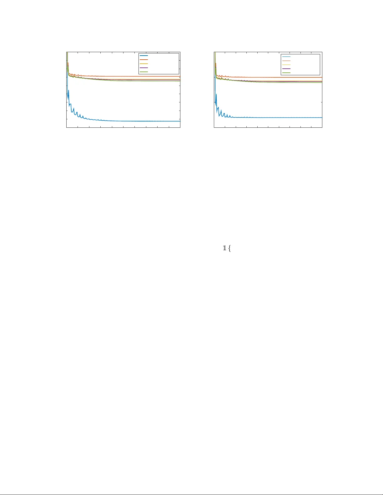
Depth-W idth T radeof fs in Approximating Natural Functions with Neural Networks Itay Safran W eizmann Institute of Science itay.safran@weizmann.ac.il Ohad Shamir W eizmann Institute of Science ohad.shamir@weizmann.ac.il Abstract W e provide sev eral new depth-based separation results for feed-forward neural networks, proving that various types of simple and natural functions can be better approximated using deeper networks than shallo wer ones, e ven if the shallower networks are much larger . This includes indicators of balls and ellipses; non-linear functions which are radial with respect to the L 1 norm; and smooth non-linear functions. W e also show that these gaps can be observed experimentally: Increasing the depth indeed allows better learning than increasing width, when training neural networks to learn an indicator of a unit ball. 1 Intr oduction Deep learning, in the form of artificial neural networks, has seen a dramatic resurgence in the past recent years, achie ving great performance impro vements in v arious fields of artificial intelligence such as computer vision and speech recognition. While empirically successful, our theoretical understanding of deep learning is still limited at best. An emerging line of recent works has studied the expr essive power of neural networks: What functions can and cannot be represented by networks of a giv en architecture (see related work section below). A particular focus has been the trade-off between the network’ s width and depth: On the one hand, it is well- kno wn that large enough networks of depth 2 can already approximate any continuous target function on [0 , 1] d to arbitrary accuracy (Cybenko, 1989; Hornik, 1991). On the other hand, it has long been evident that deeper networks tend to perform better than shallow ones, a phenomenon supported by the intuition that depth, providing compositional expressibility , is necessary for efficiently representing some functions. Indeed, recent empirical e vidence suggests that e ven at large depths, deeper networks can offer benefits ov er shallo wer networks (He et al., 2015). T o demonstrate the power of depth in neural networks, a clean and precise approach is to prov e the existence of functions which can be expressed (or well-approximated) by moderately-sized networks of a giv en depth, yet cannot be approximated well by shallower networks, ev en if their size is much larger . Ho wev er , the mere existence of such functions is not enough: Ideally , we would like to show such depth separation results using natural , interpretable functions, of the type we may e xpect neural networks to successfully train on. Pro ving that depth is necessary for such functions can gi ve us a clearer and more useful insight into what v arious neural network architectures can and cannot express in practice. In this paper, we provide several contributions to this emerging line of work. W e focus on standard, v anilla feedforward networks (using some fixed activ ation function, such as the popular ReLU), and measure 1 expressi v eness directly in terms of approximation error , defined as the e xpected squared loss with respect to some distribution o ver the input domain. In this setting, we sho w the follo wing: • W e prove that the indicator of the Euclidean unit ball, x 7→ 1 {k x k ≤ 1 } in R d , which can be easily approximated to accurac y  using a 3-layer network with O ( d/ ) neurons, cannot be approximated to an accurac y higher than O (1 /d 4 ) using a 2-layer network, unless its width is exponential in d . In f act, we show the same result more generally , for any indicator of an ellipsoid x 7→ 1 {k A x + b k ≤ r } (where A is a non-singular matrix and b is a vector). The proof is based on a reduction from the main result of Eldan & Shamir (2016), which shows a separation between 2-layer and 3-layer networks using a more complicated and less natural radial function. • W e show that this depth/width trade-of f can also be observed experimentally: Specifically , that the indicator of a unit ball can be learned quite well using a 3-layer network, using standard backpropaga- tion, b ut learning the same function with a 2-layer netw ork (e ven if much larger) is significantly more dif ficult. Our theoretical result indicates that this gap in performance is due to approximation error issues. This experiment also highlights the fact that our separation result is for a natural function that is not just well-approximated by some 3-layer network, but can also be learned well from data using standard methods. • W e prove that any L 1 radial function x 7→ f ( k x k 1 ) , where x ∈ R d and f : R → R is piece wise-linear , cannot be approximated to accuracy  by a depth 2 ReLU network of width less than ˜ Ω(min { 1 /, exp(Ω( d )) } ) . In contrast, such functions can be represented exactly by 3-layer ReLU netw orks. • Finally , we prov e that any member of a wide family of non-linear and twice-dif ferentiable functions (including for instance x 7→ x 2 in [0 , 1] ), which can be approximated to accuracy  using ReLU networks of depth and width O ( poly (log (1 / ))) , cannot be approximated to similar accuracy by constant-depth ReLU networks, unless their width is at least Ω( poly (1 / )) . W e note that a similar result appeared online concurrently and independently of ours in Y arotsky (2016); Liang & Srikant (2016), but the setting is a bit dif ferent (see related work below for more details). Related W ork The question of studying the effect of depth in neural network has receiv ed considerable attention recently , and studied under v arious settings. Many of these works consider a somewhat dif ferent setting than ours, and hence are not directly comparable. These include networks which are not plain-v anilla ones (e.g. Cohen et al. (2016); Delalleau & Bengio (2011); Martens & Medabalimi (2014)), measuring quantities other than approximation error (e.g. Bianchini & Scars elli (2014); Poole et al. (2016)), focusing only on approximation upper bounds (e.g. Shaham et al. (2016)), or measuring approximation error in terms of L ∞ -type bounds, i.e. sup x | f ( x ) − ˜ f ( x )) | rather than L 2 -type bounds E x ( f ( x ) − ˜ f ( x )) 2 (e.g. Y arotsky (2016); Liang & Srikant (2016)). W e note that the latter distinction is important: Although L ∞ bounds are more common in the approximation theory literature, L 2 bounds are more natural in the context of statistical machine learning problems (where we care about the expected loss ov er some distribution). Moreov er , L 2 approximation lo wer bounds are stronger , in the sense that an L 2 lo wer bound easily translates to a lower bound on L ∞ lo wer bound, but not vice v ersa 1 . 1 T o give a tri vial example, ReLU networks alw ays express continuous functions, and therefore can nev er approximate a dis- continuous function such as x 7→ 1 { x ≥ 0 } in an L ∞ sense, yet can easily approximate it in an L 2 sense given any continuous distribution. 2 A note worthy paper in the same setting as ours is T elgarsky (2016), which proves a separation result between the expressi vity of ReLU networks of depth k and depth o ( k / log ( k )) (for any k ). This holds e ven for one-dimensional functions, where a depth k network is sho wn to realize a saw-tooth function with exp( O ( k )) oscillations, whereas any network of depth o ( k / log ( k )) would require a width super- polynomial in k to approximate it by more than a constant. In fact, we ourselv es rely on this construction in the proofs of our results in Sec. 5. On the flip side, in our paper we focus on separation in terms of the accuracy or dimension, rather than a parameter k . Moreov er , the construction there relies on a highly oscillatory function, with Lipschitz constant exponential in k almost everywhere. In contrast, in our paper we focus on simpler functions, of the type that are likely to be learnable from data using standard methods. Our separation results in Sec. 5 (for smooth non-linear functions) are closely related to those of Y arotsk y (2016); Liang & Srikant (2016), which appeared online concurrently and independently of our work, and the proof ideas are quite similar . Howe ver , these papers focused on L ∞ bounds rather than L 2 bounds. Moreov er , Y arotsky (2016) considers a class of functions different than ours in their positiv e results, and Liang & Srikant (2016) consider networks employing a mix of ReLU and threshold acti v ations, whereas we consider a purely ReLU network. Another rele vant and insightful work is Poggio et al. (2016), which considers width vs. depth and provide general results on e xpressibility of functions with a compositional nature. Ho wev er , the focus there is on worse-case approximation over general classes of functions, rather than separation results in terms of specific functions as we do here, and the details and setting is some what orthogonal to ours. 2 Pr eliminaries In general, we let bold-faced letters such as x = ( x 1 , . . . , x d ) denote vectors, and capital letters denote matrices or probabilistic ev ents. k·k denotes the Euclidean norm, and k·k 1 the 1 -norm. 1 {·} denotes the indicator function. W e use the standard asymptotic notation O ( · ) and Ω( · ) to hide constants, and ˜ O ( · ) and ˜ Ω( · ) to hide constants and f actors logarithmic in the problem parameters. Neural Networks. W e consider feed-forward neural networks, computing functions from R d to R . The network is composed of layers of neurons, where each neuron computes a function of the form x 7→ σ ( w > x + b ) , where w is a weight vector , b is a bias term and σ : R 7→ R is a non-linear activ ation function, such as the ReLU function σ ( z ) = [ z ] + = max { 0 , z } . Letting σ ( W x + b ) be a shorthand for  σ ( w > 1 x + b 1 ) , . . . , σ ( w > n x + b n )  , we define a layer of n neurons as x 7→ σ ( W x + b ) . By denoting the output of the i th layer as O i , we can define a network of arbitrary depth recursively by O i +1 = σ ( W i +1 O i + b i +1 ) , where W i , b i represent the matrix of weights and bias of the i th layer , respectively . Follo wing a standard con vention for multi-layer networks, the final layer h is a purely linear function with no bias, i.e. O h = W h · O h − 1 . W e define the depth of the network as the number of layers l , and denote the number of neurons n i in the i th layer as the size of the layer . W e define the width of a network as max i ∈{ 1 ,...,l } n i . Finally , a ReLU network is a neural network where all the non-linear acti vations are the ReLU function. W e use “2-layer” and “3-layer” to denote networks of depth 2 and 3. In particular , in our notation a 2-layer ReLU network has the form x 7→ n 1 X i =1 v i · [ w > i x + b i ] + for some parameters v 1 , b 1 , . . . , v n 1 , b n 1 and d -dimensional vectors w 1 , . . . , w n 1 . Similarly , a 3-layer ReLU 3 network has the form n 2 X i =1 u i   n 1 X j =1 v i,j h w > i,j x + b i,j i + + c i   + for some parameters { u i , v i,j , b i,j , c i , w i,j } . A pproximation err or . Gi ven some function f on a domain X endowed with some probability distri- bution (with density function µ ), we define the quality of its approximation by some other function ˜ f as R X ( f ( x ) − ˜ f ( x )) 2 µ ( x ) d x = E x ∼ µ [( f ( x ) − ˜ f ( x )) 2 ] . W e refer to this as approximation in the L 2 -norm sense. In one of our results (Thm. 6), we also consider approximation in the L ∞ -norm sense, defined as sup x ∈X | f ( x ) − ˜ f ( x ) | . Clearly , this upper-bounds the (square root of the) L 2 approximation error defined abov e, so as discussed in the introduction, lower bounds on the L 2 approximation error (w .r .t. any distribu- tion) are stronger than lo wer bounds on the L ∞ approximation error . 3 Indicators of L 2 Balls and Ellipsoids W e begin by considering one of the simplest possible function classes on R d , namely indicators of L 2 balls (and more generally , ellipsoids). The ability to compute such functions is necessary for many useful primiti ves, for example determining if the distance between two points in Euclidean space is belo w or above some threshold (either with respect to the Euclidean distance, or a more general Mahalanobis distance). In this section, we show a depth separation result for such functions: Although the y can be easily approximated with 3-layer networks, no 2-layer network can approximate it to high accurac y w .r .t. any distribution, unless its width is exponential in the dimension. This is formally stated in the follo wing theorem: Theorem 1 (Inapproximability with 2-layer networks) . The following holds for some positive universal constants c 1 , c 2 , c 3 , c 4 , and any network employing an activation function satisfying Assumptions 1 and 2 in Eldan & Shamir (2016): F or any d > c 1 , and any non-singular matrix A ∈ R d × d , b ∈ R d and r ∈ (0 , ∞ ) , ther e exists a continuous pr obability distribution γ on R d , such that for any function g computed by a 2-layer network of width at most c 3 exp( c 4 d ) , and for the function f ( x ) = 1 {k A x + b k ≤ r } , we have Z R d ( f ( x ) − g ( x )) 2 · γ ( x ) d x ≥ c 2 d 4 . W e note that the assumptions from Eldan & Shamir (2016) are very mild, and apply to all standard acti vation functions, including ReLU, sigmoid and threshold. The formal proof of Thm. 1 (provided below) is based on a reduction from the main result of Eldan & Shamir (2016), which shows the existence of a certain radial function (depending on the input x only through its norm) and a probability distribution which cannot be expressed by a 2-layer network, whose width is less than exponential in the dimension d to more than constant accurac y . A closer look at the proof re veals that this function (denoted as ˜ g ) can be expressed as a sum of Θ( d 2 ) indicators of L 2 balls of various radii. W e argue that if we could have accurately approximated a gi ven L 2 ball indicator with respect to all distributions, then we could hav e approximated all the indicators whose sum add up to ˜ g , and hence reach a contradiction. By a linear transformation argument, we show the same contradiction would have occured if we could hav e approximated the indicators of an non-de generate ellipse with respect to any distribution. The formal proof is provided belo w: 4 Pr oof of Thm. 1. Assume by contradiction that for f as described in the theorem, and for any distribution γ , there exists a tw o-layer network ˜ f γ of width at most c 3 exp( c 4 d ) , such that Z x ∈ R d  f ( x ) − ˜ f γ ( x )  2 γ ( x ) d x ≤  ≤ c 2 d 4 . Let ˆ A and ˆ b be a d × d non-singular matrix and vector respecti vely , to be determined later . W e begin by performing a change of variables, y = ˆ A x + ˆ b ⇐ ⇒ x = ˆ A − 1 ( y − ˆ b ) , d x =    det  ˆ A − 1     · d y , which yields Z y ∈ R d  f  ˆ A − 1  y − ˆ b  − ˜ f γ  ˆ A − 1  y − ˆ b  2 · γ  ˆ A − 1  y − ˆ b  ·    det  ˆ A − 1     · d y ≤ . (1) In particular , let us choose the distribution γ defined as γ ( z ) = | det( ˆ A ) | · µ ( ˆ A z + ˆ b ) , where µ is the (continuous) distribution used in the main result of Eldan & Shamir (2016) (note that γ is indeed a distribution, since R z γ ( z ) = (det( ˆ A )) R z µ ( ˆ A z + ˆ b ) d z , which by the change of variables x = ˆ A z + ˆ b , d x = | det( ˆ A ) | d z equals R x µ ( x ) d x = 1 ). Plugging the definition of γ in Eq. (1), and using the fact that | det( ˆ A − 1 ) | · | det( ˆ A ) | = 1 , we get Z y ∈ R d  f  ˆ A − 1  y − ˆ b  − ˜ f γ  ˆ A − 1  y − ˆ b  2 · µ ( y ) d y ≤ . (2) Letting z > 0 be an arbitrary parameter, we no w pick ˆ A = z r A and ˆ b = z r b . Recalling the definition of f as x 7→ 1 {k A x + b k ≤ r } , we get that Z y ∈ R d  1 {k y k ≤ z } − ˜ f γ  r z A − 1  y − z r b  2 · µ ( y ) d y ≤ . (3) Note that ˜ f γ  r z A − 1  y − z r b  expresses a 2-layer network composed with a linear transformation of the input, and hence can be expressed in turn by a 2-layer network (as we can absorb the linear transformation into the parameters of each neuron in the first layer). Therefore, letting k f k L 2 ( µ ) = q R y f 2 ( y ) d y denote the norm in L 2 ( µ ) function space, we sho wed the following: For any z > 0 , there e xists a 2-layer network ˜ f z such that     1 {k·k ≤ z } − ˜ f z ( · )     L 2 ( µ ) ≤ √ . (4) W ith this key result in hand, we now turn to complete the proof. W e consider the function ˜ g from Eldan & Shamir (2016), for which it was prov en that no 2-layer network can approximate it w .r .t. µ to better than constant accuracy , unless its width is exponential in the dimension d . In particular ˜ g can be written as ˜ g ( x ) = n X i =1  i · 1 {k x k ∈ [ a i , b i ] } , 5 where [ a i , b i ] are disjoint interv als,  i ∈ {− 1 , +1 } , and n = Θ( d 2 ) where d is the dimension. Since ˜ g can also be written as n X i =1  i ( 1 {k x k ≤ b i } − 1 {k x k ≤ a i } ) , we get by Eq. (4) and the triangle inequality that      ˜ g ( · ) − n X i =1  i · ( ˜ f b i ( · ) − ˜ f a i ( · )      L 2 ( µ ) ≤ n X i =1 |  i |      1 {k·k ≤ b i } − ˜ f b i     L 2 ( µ ) +    1 {k·k ≤ a i } − ˜ f a i ( · )    L 2 ( µ )  ≤ 2 n √ . Ho wev er , since a linear combination of 2 n 2-layer neural networks of width at most w is still a 2-layer network, of width at most 2 nw , we get that P n i =1  i · ( ˜ f b i ( · ) − ˜ f a i ( · )) is a 2-layer netw ork, of width at most Θ( d 2 ) · c 3 exp( c 4 d ) , which approximates ˜ g to an accuracy of less than 2 n √  = Θ( d 2 ) · p c 2 /d 4 = Θ(1) · √ c 2 . Hence, by picking c 2 , c 3 , c 4 suf ficiently small, we get a contradiction to the result of Eldan & Shamir (2016), that no 2-layer network of width smaller than c exp( cd ) (for some constant c ) can approximate ˜ g to more than constant accuracy , for a sufficiently lar ge dimension d . T o complement Thm. 1, we also show that such indicator functions can be easily approximated with 3-layer networks. The argument is quite simple: Using an activ ation such as ReLU or Sigmoid, we can use one layer to approximate any Lipschitz continuous function on any bounded interval, and in particular x 7→ x 2 . Giv en a vector x ∈ R d , we can apply this construction on each coordinate x i seperately , hence approximating x 7→ k x k 2 = P d i =1 x 2 i . Similarly , we can approximate x 7→ k A x + b k for arbitrary fixed matrices A and vectors b . Finally , with a 3-layer network, we can use the second layer to compute a continuous approximation to the threshold function z 7→ 1 { z ≤ r } . Composing these two layers, we get an arbitrarily good approximation to the function x 7→ 1 {k A x + b k ≤ r } w .r .t. any continuous distribution, with the network size scaling polynomially with the dimension d and the required accuracy . In the theorem belo w , we formalize this intuition, where for simplicity we focus on approximating the indicator of the unit ball: Theorem 2 (Approximability with 3-layer networks) . Given δ > 0 , for any activation function σ satisfying Assumption 1 in Eldan & Shamir (2016) and any continuous pr obability distrib ution µ on R d , ther e exists a constant c σ dependent only on σ , a constant c µ dependent only on µ and a function g expr essible by a 3-layer network of width at most 2 c σ √ δ · max  2 c µ d 2 , 1  , such that the following holds: Z R d ( g ( x ) − 1 {k x k 2 ≤ 1 } ) 2 µ ( x ) d x ≤ δ. The proof of the theorem appears in Subsection 6.1. 6 Batch number (x1000) 0 20 40 60 80 100 120 140 160 180 200 RMSE (training set) 0.12 0.14 0.16 0.18 0.2 0.22 0.24 0.26 0.28 0.3 3-layer, width 100 2-layer, width 100 2-layer, width 200 2-layer, width 400 2-layer, width 800 Batch number (x1000) 0 20 40 60 80 100 120 140 160 180 200 RMSE (validation set) 0.15 0.2 0.25 0.3 3-layer, width 100 2-layer, width 100 2-layer, width 200 2-layer, width 400 2-layer, width 800 Figure 1: The experiment results, depicting the network’ s root mean square error ov er the training set (left) and validation set (right), as a function of the number of batches processed. Best vie wed in color . 3.1 An Experiment In this subsection, we empirically demonstrate that indicator functions of balls are indeed easier to learn with a 3-layer network, compared to a 2-layer network (ev en if the 2-layer network is significantly larger). This indicates that the depth/width trade-off for indicators of balls, predicted by our theory , can indeed be observed experimentally . Moreo ver , it highlights the fact that our separation result is for simple natural functions, that can be learned reasonably well from data using standard methods. For our experiment, we sampled 5 · 10 5 data instances in R 100 , with a direction chosen uniformly at random and a norm drawn uniformly at random from the interval [0 , 2] . T o each instance, we associated a target value computed according to the target function f ( x ) = 1 {k x k 2 ≤ 1 } . Another 5 · 10 4 examples were generated in a similar manner and used as a v alidation set. W e trained 5 ReLU netw orks on this dataset: • One 3-layer network, with a first hidden layer of size 100 , a second hidden layer of size 20 , and a linear output neuron. • Four 2-layer netw orks, with hidden layer of sizes 100 , 200 , 400 and 800 , and a linear output neuron. T raining was performed with backpropagation, using the T ensorFlo w library . W e used the squared loss ` ( y , y 0 ) = ( y − y 0 ) 2 and batches of size 100. For all networks, we chose a momentum parameter of 0.95, and a learning rate starting at 0.1, decaying by a multiplicativ e factor of 0.95 ev ery 1000 batches, and stopping at 10 − 4 . The results are presented in Fig. 1. As can be clearly seen, the 3-layer network achiev es significantly better performance than the 2-layer networks. This is true ev en though some of these networks are signifi- cantly larger and with more parameters (for example, the 2-layer , width 800 network has ˜80K parameters, vs. ˜10K parameters for the 3-layer network). This gap in performance is the exact opposite of what might be expected based on parameter counting alone. Moreov er , increasing the width of the 2-layer networks exhibits diminishing returns: The performance impro vement in doubling the width from 100 to 200 is much larger than doubling the width from 200 to 400 or 400 to 800. This indicates that one would need a much larger 2-layer network to match the 3-layer , width 100 network’ s performance. Thus, we conclude that the network’ s depth indeed plays a crucial role, and that 3-layer networks are inherently more suitable to e xpress indicator functions of the type we studied. 7 4 L 1 Radial Functions; ReLU Networks Having considered functions depending on the L 2 norm, we now turn to consider functions depending on the L 1 norm. Focusing on ReLU networks, we will show a certain separation result holding for any non-linear function, which depends on the input x only via its 1-norm k x k 1 . Theorem 3. Let f : [0 , ∞ ) 7→ R be a function suc h that for some r , δ > 0 and  ∈ (0 , 1 / 2) , inf a,b ∈ R E x uniform on [ r, (1+  ) r ] [( f ( x ) − ( ax − b )) 2 ] > δ . Then ther e exists a distribution γ over { x : k x k 1 ≤ (1 +  ) r } , such that if a 2-layer ReLU network F ( x ) satisfies Z x ( f ( k x k 1 ) − F ( x )) 2 γ ( x ) d x ≤ δ / 2 , then its width must be at least ˜ Ω(min { 1 /, exp(Ω( d )) } ) (wher e the ˜ Ω notation hides constants and factors logarithmic in , d ). T o gi ve a concrete example, suppose that f ( z ) = [ z − 1] + , which cannot be approximated by a linear function better than O (  2 ) in an  -neighborhood of 1 . By taking r = 1 −  2 and δ = O (  2 ) , we get that no 2- layer network can approximate the function [ k x k 1 − 1] + (at least with respect to some distribution), unless its width is ˜ Ω(min { 1 /, exp(Ω( d )) } ) . On the flip side, f ( k x k 1 ) can be expressed exactly by a 3-layer , width 2 d ReLU network: x 7→ [ P d i =1 ([ x i ] + + [ − x i ] + ) − 1] + , where the output neuron is simply the identity function. The same argument would work for any piecewise-linear f . More generally , the same kind of argument would work for any function f exhibiting a non-linear behavior at some points: Such functions can be well-approximated by 3-layer networks (by approximating f with a piece wise-linear function), yet any approximating 2-layer netw ork will hav e a lower bound on its size as specified in the theorem. Intuiti vely , the proof relies on showing that any good 2 -layer approximation of f ( k x k 1 ) must capture the non-linear behavior of f close to “most” points x satisfying k x k 1 ≈ r . Howe ver , a 2 -layer ReLU network x 7→ P N j =1 a j [ h w j , x i + b j ] + is piecewise linear , with non-linearities only at the union of the N hyperplanes ∪ j { x : h w j , x i + b j = 0 } . This implies that “most” points x s.t. k x k 1 ≈ r must be  -close to a hyperplane { x : h w j , x i + b j = 0 } . Howe ver , the geometry of the L 1 ball { x : k x k = r } is such that the  neighborhood of any single hyperplane can only cover a “small” portion of that ball, yet we need to cover most of the L 1 ball. Using this and an appropriate construction, we sho w that required number of hyperplanes is at least 1 / , as long as  > exp( −O ( d )) (and if  is smaller than that, we can simply use one neuron/hyperplane for each of the 2 d facets of the L 1 ball, and get a cov ering using 2 d neurons/hyperplanes). The formal proof appears in Subsection 6.2. W e note that the bound in Thm. 3 is of a weaker nature than the bound in the pre vious section, in that the lo wer bound is only polynomial rather than exponential (albeit w .r .t. dif ferent problem parameters:  vs. d ). Nevertheless, we belie ve this does point out that L 1 balls also pose a geometric dif ficulty for 2-layer networks, and conjecture that our lower bound can be considerably improved: Indeed, at the moment we do not know how to approximate a function such as x 7→ [ k x k 1 − 1] + with 2-layer networks to better than constant accuracy , using less than Ω(2 d ) neurons. 5 C 2 Nonlinear Functions; ReLU Networks In this section, we establish a depth separation result for approximating continuously twice-differentiable ( C 2 ) functions using ReLU neural networks. Unlike the previous results in this paper , the separation is for 8 depths which can be larger than 3, depending on the required approximation error . Also, the results will all be with respect to the uniform distribution µ d ov er [0 , 1] d . As mentioned earlier, the results and techniques in this section are closely related to the independent results of Y arotsk y (2016); Liang & Srikant (2016), b ut our emphasis is on L 2 rather than L ∞ approximation bounds, and we focus on somewhat dif ferent network architectures and function classes. Clearly , not all C 2 functions are dif ficult to approximate (e.g. a linear function can be e xpressed exactly with a 2-layer network). Instead, we consider functions which hav e a certain degree of non-linearity , in the sense that its Hessians are non-zero along some direction, on a significant portion of the domain. Formally , we make the follo wing definition: Definition 1. Let µ d denote the uniform distribution on [0 , 1] d . F or a function f : [0 , 1] d → R and some λ > 0 , denote σ λ ( f ) = sup v ∈ S d − 1 , U ∈U s.t. v > H ( f )( x ) v ≥ λ ∀ x ∈ U µ d ( U ) , wher e S d − 1 = { x : k x k 2 = 1 } is the d -dimensional unit hyperspher e, and U is the set of all connected and measurable subsets of [0 , 1] d . In words, σ λ ( f ) is the measure (w .r .t. the uniform distribution on [0 , 1] d ) of the largest connected set in the domain of f , where at any point, f has curvature at least λ along some fixed direction v . The “prototypical” functions f we are interested in is when σ λ ( f ) is lo wer bounded by a constant (e.g. it is 1 if f is strongly con ve x). W e stress that our results in this section will hold equally well by considering the condition v > H ( f )( x ) v ≤ − λ as well, ho wev er for the sake of simplicity we focus on the former condition appearing in Def. 1. Our goal is to sho w a depth separation result inidividually for any such function (that is, for any such function, there is a gap in the attainable error between deeper and shallower netw orks, ev en if the shallo w network is considerably larger). As usual, we start with an inapproximability result. Specifically , we prove the follo wing lower bound on the attainable approximation error of f , using a ReLU neural network of a giv en depth and width: Theorem 4. F or any C 2 function f : [0 , 1] d → R , any λ > 0 , and any function g on [0 , 1] d expr essible by a ReLU network of depth l and maximal width m , it holds that Z [0 , 1] d ( f ( x ) − g ( x ) 2 µ d ( x ) d x ≥ c · λ 2 · σ 5 λ (2 m ) 4 l , wher e c > 0 is a universal constant. The theorem con veys a ke y tradeoff between depth and width when approximating a C 2 function using ReLU netw orks: The error cannot decay faster than polynomially in the width m , yet the bound deteriorates exponentially in the depth l . As we sho w later on, this deterioration does not stem from the looseness in the bound: For well-behav ed f , it is indeed possible to construct ReLU networks, where the approximation error decays exponentially with depth. The proof of Thm. 4 appears in Subsection 6.3, and is based on a series of intermediate results. First, we show that any strictly curved function (in a sense similar to Definition 1) cannot be well-approximated in an L 2 sense by piecewise linear functions, unless the number of linear regions is large. T o that end, we first establish some necessary tools based on Legendre polynomials. W e then prove a result specific to the one-dimensional case, including an explicit lower bound if the target function is quadratic (Thm. 9) or strongly con ve x or concave (Thm. 10). W e then expand the construction to get an error lower bound 9 Figure 2: ReLU approximation of the function x 7→ x 2 obtained by extracting 5 bits. The number of linear segments gro ws exponentially with the number of bits and the approximating network size. in general dimension d , depending on the number of linear regions in the approximating piece wise-linear function. Finally , we note that any ReLU network induces a piece wise-linear function, and bound the number of linear regions induced by a ReLU network of a giv en width and depth (using a lemma borrowed from T elgarsky (2016)). Combining this with the previous lo wer bound yields Thm. 4. W e now turn to complement this lo wer bound with an approximability result, showing that with more depth, a wide family of functions to which Thm. 4 applies can be approximated with exponentially high accuracy . Specifically , we consider functions which can be approximated using a moderate number of multiplications and additions, where the v alues of intermediate computations are bounded (for example, a special case is any function approximable by a moderately-sized Boolean circuit, or a polynomial). The k ey result to sho w this is the follo wing, which implies that the multiplication of two (bounded-size) numbers can be approximated by a ReLU network, with error decaying e xponentially with depth: Theorem 5. Let f : [ − M , M ] 2 → R , f ( x, y ) = x · y and let  > 0 be arbitrary . Then e xists a ReLU neural network g of width 4  log  M   + 13 and depth  2 log  M   + 9 satisfying sup ( x,y ) ∈ [ − M ,M ] 2 | f ( x, y ) − g ( x, y ) | ≤ . The idea of the construction is that depth allo ws us to compute highly-oscillating functions, which can extract high-order bits from the binary representation of the inputs. Gi ven these bits, one can compute the product by a procedure resembling long multiplication, as sho wn in Fig. 2, and formally prov en as follo ws: Pr oof of Thm. 5. W e begin by observing that by using a simple linear change of variables on x , we may assume without loss of generality that x ∈ [0 , 1] , as we can just rescale x to the interval [0 , 1] , and then map it back to its original domain [ − M , M ] , where the error will multiply by a factor of 2 M . Then by requiring accuracy  2 M instead of  , the result will follo w . 10 The ke y behind the proof is that performing bit-wise operations on the first k bits of x ∈ [0 , 1] yields an estimation of the product to accuracy 2 1 − k M . Let x = P ∞ i =1 2 − i x i be the binary representation of x where x i is the i th bit of x , then x · y = ∞ X i =1 2 − i x i · y = k X i =1 2 − i x i · y + ∞ X i = k +1 2 − i x i · y . (5) But since      ∞ X i = k +1 2 − i x i · y      ≤      ∞ X i = k +1 2 − i · y      = 2 − k | y | ≤ 2 1 − k M , Eq. (5) implies      x · y − k X i =1 2 − i x i · y      ≤ 2 1 − k M . Requiring that 2 2 − k M ≤  2 M , it suf fices to sho w the existence of a network which approximates the function P k i =1 2 − i x i · y to accurac y  2 , where k = 2  log  8 M   . This way both approximations will be at most  2 , resulting in the desired accuracy of  . Before specifying the architecture which e xtracts the i th bit of x , we first describe the last 2 layers of the network. Let the penultimate layer comprise of k neurons, each recei ving both y and x i as input, and having the set of weights  2 − i , 1 , − 1  . Thus, the output of the i th neuron in the penultimate layer is  2 − i y + x i − 1  + = 2 − i x i y . Let the final single output neuron have the set of weights (1 , . . . , 1 , 0) ∈ R k +1 , this way , the output of the network will be P k i =1 2 − i x i · y as required. W e now specify the architecture which e xtracts the first most significant k bits of x . In T elgarsky (2016), the author demonstrates ho w the composition of the function ϕ ( x ) = [2 x ] + − [4 x − 2] + with itself i times, ϕ i , yields a highly oscillatory triangle wa ve function in the domain [0 , 1] . Furthermore, we observe that ϕ ( x ) = 0 ∀ x ≤ 0 , and thus ϕ i ( x ) = 0 ∀ x ≤ 0 . Now , a linear shift of the input of ϕ i by 2 − i − 1 , and composing the output with σ δ ( x ) =  1 2 δ x − 1 4 δ + 1 2  + −  1 2 δ x − 1 4 δ − 1 2  + , which con v erges to x 7→ 1 { x ≥ 0 . 5 } as δ → 0 , results in an approximation of x 7→ x i : σ δ  ϕ i  x − 2 − i − 1  . W e stress that choosing δ such that the network approximates the bit-wise product to accuracy  2 will require δ to be of magnitude 1  , but this poses no problem as representing such a number requires log  1   bits, which is also the magnitude of the size of the network, as suggested by the follo wing analysis. 11 Next, we compute the size of the network required to implement the above approximation. T o compute ϕ only two neurons are required, therefore ϕ i can be computed using i layers with 2 neurons in each, and finally composing this with σ δ requires a subsequent layer with 2 more neurons. T o implement the i th bit extractor we therefore require a network of size 2 × ( i + 1) . Using dummy neurons to propagate the i th bit for i < k , the architecture extracting the k most significant bits of x will be of size 2 k × ( k + 1) . Adding the final component performing the multiplication estimation will require 2 more layers of width k and 1 respecti vely , and an increase of the width by 1 to propagate y to the penultimate layer , resulting in a network of size (2 k + 1) × ( k + 1) . Thm. 5 shows that multiplication can be performed very accurately by deep networks. Moreov er , addi- tions can be computed by ReLU networks exactly , using only a single layer with 4 neurons: Let α , β ∈ R be arbitrary , then ( x, y ) 7→ α · x + β · y is giv en in terms of ReLU summation by α [ x ] + − α [ − x ] + + β [ y ] + − β [ − y ] + . Repeating these arguments, we see that any function which can be approximated by a bounded number of operations inv olving additions and multiplications, can also be approximated well by moderately-sized networks. This is formalized in the follo wing theorem, which provides an approximation error upper bound (in the L ∞ sense, which is stronger than L 2 for upper bounds): Theorem 6. Let F t,M , be the family of functions on the domain [0 , 1] d with the pr operty that f ∈ F t,M , is appr oximable to accuracy  with r espect to the infinity norm, using at most t operations in volving weighted addition, ( x, y ) 7→ α · x + β · y , wher e α, β ∈ R ar e fixed; and multiplication, ( x, y ) 7→ x · y , where each intermediate computation stage is bounded in the interval [ − M , M ] . Then there e xists a universal constant c , and a ReLU network g of width and depth at most c  t log  1   + t 2 log ( M )  , such that sup x ∈ [0 , 1] d | f ( x ) − g ( x ) | ≤ 2 . As discussed in Sec. 2, this type of L ∞ approximation bound implies an L 2 approximation bound with respect to any distrib ution. The proof of the theorem appears in Subsection 6.4. Combining Thm. 4 and Thm. 6, we can state the following corollary , which formally sho ws how depth can be exponentially more v aluable than width as a function of the tar get accuracy  : Corollary 1. Suppose f ∈ C 2 ∩F t (  ) ,M (  ) , , wher e t (  ) = O ( poly (log (1 / ))) and M (  ) = O ( poly (1 / )) . Then appr oximating f to accuracy  in the L 2 norm using a fixed depth ReLU network r equir es width at least poly (1 / ) , whereas ther e exists a ReLU network of depth and width at most p (log (1 / )) which ap- pr oximates f to accuracy  in the infinity norm, wher e p is a polynomial depending solely on f . Pr oof. The lo wer bound follows immediately from Thm. 4. For the upper bound, observ e that Thm. 6 implies an  approximation by a netw ork of width and depth at most c  t ( / 2) log (2 / ) + ( t ( / 2)) 2 log ( M ( / 2))  , which by the assumption of Corollary 1, can be bounded by p (log (1 / )) for some polynomial p which depends solely on f . 12 Acknowledgements This research is supported in part by an FP7 Marie Curie CIG grant, Israel Science F oundation grant 425/13, and the Intel ICRI-CI Institute. W e would like to thank Shai Shalev-Shwartz for some illuminating discus- sions, Eran Amar for his v aluable help with the experiment, and Lv Xianzhang for spotting a mistake in a pre vious version of Sec. 3. Refer ences Bianchini, M. and Scarselli, F . On the complexity of shallow and deep neural network classifiers. In ESANN , 2014. Cohen, Nadav , Sharir , Or , and Shashua, Amnon. On the expressi ve power of deep learning: A tensor analysis. In 29th Annual Confer ence on Learning Theory , pp. 698–728, 2016. Cybenko, Geor ge. Approximation by superpositions of a sigmoidal function. Mathematics of contr ol, signals and systems , 2(4):303–314, 1989. Delalleau, O. and Bengio, Y . Shallow vs. deep sum-product netw orks. In NIPS , pp. 666–674, 2011. Eldan, Ronen and Shamir , Ohad. The power of depth for feedforward neural networks. In 29th Annual Confer ence on Learning Theory , pp. 907–940, 2016. He, Kaiming, Zhang, Xiangyu, Ren, Shaoqing, and Sun, Jian. Deep residual learning for image recognition. arXiv pr eprint arXiv:1512.03385 , 2015. Hornik, Kurt. Approximation capabilities of multilayer feedforward networks. Neural networks , 4(2):251– 257, 1991. Liang, Shiyu and Srikant, R. Why deep neural networks? arXiv pr eprint arXiv:1610.04161 , 2016. Martens, J. and Medabalimi, V . On the expressi ve efficiency of sum product networks. arXiv preprint arXiv:1411.7717 , 2014. Poggio, T omaso, Mhaskar , Hrushikesh, Rosasco, Lorenzo, Miranda, Brando, and Liao, Qianli. Why and when can deep–but not shallo w–networks av oid the curse of dimensionality: a revie w . arXiv preprint arXiv:1611.00740 , 2016. Poole, Ben, Lahiri, Subhaneil, Raghu, Maithreyi, Sohl-Dickstein, Jascha, and Ganguli, Surya. Exponen- tial expressi vity in deep neural networks through transient chaos. In Advances In Neural Information Pr ocessing Systems , pp. 3360–3368, 2016. Shaham, Uri, Cloninger , Alexander , and Coifman, Ronald R. Pro vable approximation properties for deep neural networks. Applied and Computational Harmonic Analysis , 2016. T elgarsky , Matus. Benefits of depth in neural networks. arXiv preprint , 2016. Y arotsk y , Dmitry . Error bounds for approximations with deep relu networks. arXiv pr eprint arXiv:1610.01145 , 2016. 13 6 Pr oofs 6.1 Proof of Thm. 2 This proof bears resemblance to the proof provided in Eldan & Shamir (2016)[Lemma 10], albeit once approximating k x k 2 2 , the follo wing construction takes a slightly different route. For completeness, we also state assumption 1 from Eldan & Shamir (2016): Assumption 1. Given the activation function σ , ther e is a constant c σ ≥ 1 (depending only on σ ) such that the following holds: F or any L -Lipschitz function f : R → R which is constant outside a bounded interval [ − R, R ] , and for any δ , ther e e xist scalars a, { α i , β i , γ i } w i =1 , wher e w ≤ c σ RL δ , such that the function h ( x ) = a + w X i =1 α i · σ ( β i x − γ i ) satisfies sup x ∈ R | f ( x ) − h ( x ) | ≤ δ. As discussed in Eldan & Shamir (2016), this assumption is satisfied by ReLU, sigmoid, threshold, and more generally all standard acti vation functions we are f amiliar with. Pr oof. Consider the 1 -Lipschitz function l ( x ) = min  x 2 , 1  , which is constant outside [ − 1 , 1] , as well as the function ` ( x ) = d X i =1 l ( x i ) = d X i =1 min  x 2 i , 1  on R d . Applying assumption 1, we obtain a function ˜ l ( x ) ha ving the form a + P w i =1 α i σ ( β i x − γ i ) so that sup x ∈ R    ˜ l ( x ) − l ( x )    ≤ δ 1 d , and where the width parameter w is at most c σ d δ 1 . Consequently , the function ˜ ` ( x ) = d X i =1 ˜ l ( x i ) can be expressed in the form a + P w i =1 α i σ ( β i x − γ i ) where w ≤ c σ d 2 δ 1 , yielding an approximation satisfying sup x ∈ R d    ˜ ` ( x ) − ` ( x )    ≤ δ 1 . (6) W e now in vok e assumption 1 again to approximate the 1 -Lipschitz function f ( x ) =      1 x < 0 1 − x x ∈ [0 , 1] 0 x > 1 14 and obtain an approximation ˜ f ( x ) = ˜ a + P ˜ w i =1 ˜ α i σ  ˜ β i x − ˜ γ i  satisfying sup x ∈ R    ˜ f ( x ) − f ( x )    ≤ δ 2 (7) where ˜ w ≤ c σ / 2 δ 2 . No w consider the composition g = ˜ f ◦  c µ · ˜ ` − c µ  , where c µ > 0 depends on µ , to be determined later . This composition has the form a + w X i =1 u i σ   w X j =1 v i,j σ ( h w i,j , x i + b i,j ) + c i   for appropriate scalars a, u i , c i , v i,j , b i,j and vectors w i,j , and where w is at most max  c σ d 2 /δ 1 , c σ / 2 δ 2  . It is no w left to bound the approximation error obtained by g . W e hav e k g − 1 {k x k 2 ≤ 1 }k L 2 ( µ ) ≤ k g − f ◦ ( c µ − c µ · ` ) k L 2 ( µ ) + k f ◦ ( c µ − c µ · ` ) − 1 {k x k 2 ≤ 1 }k L 2 ( µ ) . (8) Beginning with the second summand, define for an y  > 0 , R  = n x ∈ R d : 1 −  ≤ k x k 2 2 ≤ 1 o . Since µ is continuous, there e xists  ∈ (0 , 1) such that Z R  µ ( x ) d x ≤ √ δ 2 . (9) W e hav e for any x ∈ R d satisfying 1 ≤ k x k 2 2 that ` ( x ) = 1 and therefore f ◦ ( c µ − c µ · ` ) ( x ) = 1 . (10) T aking c µ = 1 / , we hav e for any x ∈ R d satisfying k x k 2 2 ≤ 1 −  that f ◦ ( c µ − c µ · ` ) ( x ) ≤ f  1  − 1  (1 −  )  = f (1) = 0 (11) Combining both Eq. (10) and Eq. (11) we compute Z R d ( f ( c µ − c µ · ` ( x )) − 1 {k x k 2 ≤ 1 } ) 2 µ ( x ) d x = Z R  ( f ( c µ − c µ · ` ( x )) − 1 {k x k 2 ≤ 1 } ) 2 µ ( x ) d x ≤ Z R  1 · µ ( x ) d x ≤ √ δ 2 , (12) where the equality is since both functions are equal outside of R  , the first inequality is since the difference between the two functions on R  is at most 1 , and the last inequality is due to Eq. (9). Moving to the first 15 summand in Eq. (8), we hav e k g − f ◦ ( c µ − c µ · ` ) k L 2 ( µ ) ≤ k g − f ◦ ( c µ − c µ · ` ) k ∞ ≤    g − f ◦  c µ − c µ · ˜ `     ∞ +    f ◦  c µ − c µ · ˜ `  − f ◦ ( c µ − c µ · ` )    ∞ ≤ δ 2 +     c µ − c µ · ˜ `  − ( c µ − c µ · ` )    ∞ ≤ δ 2 + c µ    ˜ ` − `    ∞ ≤ δ 2 + c µ δ 1 , where the third inequality is due to Eq. (7) and f being 1 -Lipschitz and the last inequality due to Eq. (6). Letting δ 2 = √ δ / 4 and δ 1 = √ δ / 4 c µ which also entails w ≤ 2 c σ √ δ · max  2 c µ d 2 , 1  , the abov e is upper bounded by √ δ / 2 , which when combined with Eq. (12) and plugged in Eq. (8) implies the lemma. 6.2 Proof of Thm. 3 Consider an input distribution of the form x = sr v , where v is drawn from a certain distribution on the unit L 1 sphere { x : k x k 1 = 1 } to be specified later , and s is uniformly distrib uted on [1 , 1 +  ] . Let F ( x ) = N X j =1 a j [ h w j , x i + b j ] + be a 2-layer ReLU network of width N , such that with respect to the distribution abov e, E x  ( f ( k x k 1 ) − F ( x )) 2  = E v  E s  ( f ( sr ) − F ( sr v )) 2   v  ≤ δ  2 . By Marko v’ s inequality , this implies Pr v  E s  f ( sr ) − F ( sr v ) 2   v  ≤ δ   ≥ 1 2 . By the assumption on f , and the f act that s is uniform on [1 , 1 +  ] , we hav e that E s  f ( sr ) − F ( sr v ) 2   v  ≤ δ  only if ˜ f N is not a linear function on the line between r v and (1 +  ) r v . In other words, this line must be crossed by the hyperplane { x : h w j , x i + b j = 0 } for some neuron j . Thus, we must hav e Pr v ( ∃ j ∈ { 1 , . . . , N } , s ∈ [1 , 1 +  ] s.t. h w j , sr v i + b j = 0) ≥ 1 2 . (13) 16 The left hand side equals Pr v ( ∃ j ∈ { 1 . . . N } , s ∈ [1 , 1 +  ] s.t. h w j , v i = − b j /sr ) = Pr v  ∃ j ∈ { 1 . . . N } s.t. h w j , v i between − b j r and − b j (1 +  ) r  ≤ Pr v  ∃ j ∈ { 1 . . . N } s.t. h w j , v i betwen − b j r and − (1 −  ) b j r  ≤ N X j =1 Pr v  h w j , v i between − b j r and − (1 −  ) b j r  ≤ N · sup w ∈ R d ,b ∈ R Pr v  h w , v i between − b r and − (1 −  ) b r  = N · sup w ∈ R d ,b ∈ R Pr v  − r w b , v  ∈ [1 − , 1]  = N · sup w ∈ R d Pr v ( h w , v i ∈ [1 − , 1]) , where in the first inequality we used the fact that 1 1+  ≥ 1 −  for all  ∈ (0 , 1) , and in the second inequality we used a union bound. Combining these inequalities with Eq. (13), we get that N ≥ 1 sup w Pr v ( h w , v i ∈ [1 − , 1]) . As a result, to prove the theorem, it is enough to construct a distribution for v on the on the unit L 1 ball, such that for any w , Pr v ( h w , v i ∈ [1 − , 1]) ≤ ˜ O (  + exp( − Ω( d ))) (14) By the inequality abov e, we would then get that N = ˜ Ω(min { 1 /, exp(Ω( d )) } ) . Specifically , consider a distribution over v defined as follows: First, we sample σ ∈ {− 1 , +1 } d uni- formly at random, and n ∈ R d from a standard Gaussian distribution, and define ˆ v = 1 d  σ + c d  I − 1 d σ σ >  n  , where c d > 0 is a parameter dependent on d to be determined later . It is easily verified that h σ /d, ˆ v i = h σ /d, σ /d i independent of n , hence ˆ v lies on the hyperplane containing the facet of the L 1 ball on which σ /d resides. Calling this facet F σ , we define v to hav e the same distribution as ˆ v , conditioned on ˆ v ∈ F σ . W e begin by ar guing that Pr v ( h w , v i ∈ [1 − , 1]) ≤ 2 · Pr ˆ v ( h w , ˆ v i ∈ [1 − , 1]) . (15) T o see this, let A = { x : h w , x i ∈ [1 − , 1] } , and note that the left hand side equals Pr( v ∈ A ) = E σ [Pr( v ∈ A | σ )] = E σ [Pr ( ˆ v ∈ A | σ , ˆ v ∈ F σ )] = E σ  Pr( ˆ v ∈ A ∩ F σ | σ ) Pr( ˆ v ∈ F σ | σ )  ≤ 1 min σ Pr( ˆ v ∈ F σ | σ ) E σ [Pr( ˆ v ∈ A | σ )] = Pr( ˆ v ∈ A ) min σ Pr( ˆ v ∈ F σ | σ ) . 17 Therefore, to prov e Eq. (15), it is enough to prov e that Pr( ˆ v ∈ F σ | σ ) ≥ 1 / 2 for an y σ . As sho wn earlier , ˆ v lies on the hyperplane containing F σ , the facet of the L 1 ball in which σ /d resides. Thus, ˆ v can be outside F σ , only if at least one of its coordinates has a dif ferent sign than σ . By definition of ˆ v , this can only happen if   c d ( I − σ σ > /d ) n   ∞ ≥ 1 . The probability of this e vent (o ver the random dra w of n ) equals Pr  max j ∈{ 1 ...d }     c d  n j − 1 d h σ , n i σ j      ≥ 1  = Pr max j ∈{ 1 ...d }      n j − σ j · 1 d d X i =1 σ i n i      ≥ 1 c d ! . Since σ i ∈ {− 1 , 1 } for all i , the ev ent on the right hand side can only occur if | n j | ≥ 1 / 2 c d for some j . Recalling that each n j has a standard Gaussian distribution, this probability can be upper bounded by Pr  max j ∈{ 1 ...d } | n j | ≥ 1 2 c d  ≤ d · Pr  | n 1 | ≥ 1 2 c d  = 2 d · Pr  n 1 ≥ 1 2 c d  ≤ 2 d · exp  − 1 4 c 2 d  , where we used a union bound and a standard Gaussian tail bound. Thus, by picking c d = s 1 4 log(4 d ) , we can ensure that the probability is at most 1 / 2 , hence proving that Pr( ˆ v ∈ F σ | σ ) ≥ 1 / 2 and vali dating Eq. (15). W ith Eq. (15) in hand, we no w turn to upper bound Pr ( h w , ˆ v i ∈ [1 − , 1]) = Pr  1 d  w , σ + c d  I − 1 d σ σ >  n  ∈ [1 − , 1]  . By the equation abov e, we hav e that conditioned on σ , the distribution of h w , ˆ v i is Gaussian with mean h σ , w i /d and v ariance c 2 d d 2 · w >  I − 1 d σ σ >  2 w = c 2 d d 2 · k w k 2 − h w , σ i 2 d ! =  c d k w k d  2 · 1 − 1 d  w k w k , σ  2 ! . By Hoef fding’ s inequality , we have that for an y t > 0 , Pr σ      h σ , w i d     > t · k w k d  ≤ 2 exp( − 2 t 2 ) and Pr σ      w k w k , σ      > r d 2 ! ≤ 2 exp( − d ) . This means that with probability at least 1 − 2 exp( − d ) − 2 exp( − 2 t 2 ) ov er the choice of σ , the distribution of h w , ˆ v i (conditioned on σ ) is Gaussian with mean bounded in absolute value by t k w k /d , and variance of at least  c d k w k d  2 ·  1 − 1 d · d 2  = 1 2  c d k w k d  2 . T o continue, we utilize the following lemma: Lemma 1. Let n be a Gaussian random variable on R with mean µ and variance v 2 for some v > 0 . Then for any  ∈ (0 , 1) , Pr ( n ∈ [1 − , 1]) ≤ r 2 π · max  1 , | µ | v  ·  1 −  . 18 Pr oof. Since the probability can only increase if we replace the mean µ by | µ | , we will assume without loss of generality that µ ≥ 0 . By definition of a Gaussian distribution, and using the easily-verified fact that exp( − z 2 ) ≤ min { 1 , 1 /z } for all z ≥ 0 , the probability equals 1 √ 2 π v 2 Z 1 1 −  exp  − ( x − µ ) 2 v 2  dx ≤  √ 2 π v 2 · max x ∈ [1 − , 1] exp  − ( x − µ ) 2 v 2  ≤  √ 2 π v 2 · max x ∈ [1 − , 1] min  1 , v | x − µ |  =  √ 2 π · max x ∈ [1 − , 1] min  1 v , 1 | x − µ |  =  √ 2 π · max x ∈ [1 − , 1] 1 max { v , | x − µ |} =  √ 2 π · max x ∈ [1 − , 1] max { 1 , µ v } max { 1 , µ v } · max { v , | x − µ |} ≤  √ 2 π · max x ∈ [1 − , 1] max { 1 , µ v } max { µ, | x − µ |} =  √ 2 π · max { 1 , µ v } max { µ, min x ∈ [1 − , 1] | x − µ |} A simple case analysis re veals that the denominator is at least 2 1 −  2 , from which the result follo ws. Using this lemma and the previous observations, we get that with probability at least 1 − 2 exp( − d ) − 2 exp( − 2 t 2 ) o ver the choice of σ , Pr( h w , ˆ v i ∈ [1 − , 1] | σ ) ≤ r 2 π · max  1 , t k w k /d c d k w k / √ 2 d  ·  1 −  = r 2 π · max  1 , t c d √ 2  ·  1 −  . Letting E be the ev ent that σ is such that this inequality is satisfied (and noting that its probability of non-occurence is at most 2 exp( − d ) + 2 exp( − 2 t 2 ) ), we get ov erall that Pr( h w , ˆ v i ∈ [1 − , 1]) = Pr( E ) · Pr( h w , ˆ v i ∈ [1 − , 1] | E ) + Pr( ¬ E ) · Pr( h w , ˆ v i ∈ [1 − , 1] |¬ E ) ≤ 1 · Pr( h w , ˆ v i ∈ [1 − , 1] | E ) + Pr( ¬ E ) · 1 ≤ r 2 π · max  1 , t c d √ 2  ·  1 −  + 2 exp( − d ) + 2 exp( − 2 t 2 ) . Recalling Eq. (15) and the definition of c d , we get that Pr( h w , v i ∈ [1 − , 1]) ≤ r 8 π · max n 1 , t · p 2 log(4 d ) o ·  1 −  + 2 exp( − d ) + 2 exp( − 2 t 2 ) . Picking t = q 1 2 log  1 −    , we get the bound r 8 π · max ( 1 , s log  1 −    log(4 d ) ) + 2 ! ·  1 −  + 2 exp( − d ) = ˜ O (  + exp( − d )) . This justifies Eq. (14), from which the result follo ws. 2 If µ ∈ [1 − , 1] , then we get max { µ, 0 } = µ ≥ 1 −  . If µ > 1 , we get max { µ, µ − 1 } > 1 ≥ 1 −  . If µ < 1 −  , we get max { µ, 1 −  − µ } ≥ (1 −  ) / 2 . 19 6.3 Proof of Thm. 4 The proof rests largely on the follo wing key result: Theorem 7. Let G n be the family of piece-wise linear functions on the domain [0 , 1] comprised of at most n linear se gments. Let G d n be the family of piece-wise linear functions on the domain [0 , 1] d , with the pr operty that for any g ∈ G d n and any affine tr ansformation h : R → R d , g ◦ h ∈ G n . Suppose f : [0 , 1] d → R is C 2 . Then for all λ > 0 inf g ∈G d n Z [0 , 1] d ( f − g ) 2 dµ d ≥ c · λ 2 · σ λ ( f ) 5 n 4 , wher e c = 5 4096 . Thm. 7 establishes that the error of a piece-wise linear approximation of a C 2 function cannot decay faster than quartically in the number of linear segments of any one-dimensional projection of the approxi- mating function. Note that this result is stronger than a bound in terms of the total number of linear regions in R d , since that number can be exponentially higher (in the dimension) than n as defined in the theorem. Before proving Thm. 7, let us explain ho w we can use it to prove Thm. 4. T o that end, we use the result in T elgarsky (2016, Lemma 3.2), of which the follo wing is an immediate corollary: Corollary 2. Let N d m,l denote the family of ReLU neural networks r eceiving input of dimension d and having depth l and maximal width m . Then N d m,l ⊆ G d (2 m ) l . Combining this corollary with Thm. 7, the result follows. The remainder of this subsection will be de voted to pro ving Thm. 7. 6.3.1 Some T echnical T ools Definition 2. Let P i denote the i th Le gendr e P olynomial given by Rodrigues’ formula: P i ( x ) = 1 2 i i ! d i dx i h  x 2 − 1  i i . These polynomials are useful for the follo wing analysis since they obe y the orthogonality relationship Z 1 − 1 P i ( x ) P j ( x ) dx = 2 2 i + 1 δ ij . Since we are interested in approximations on small interv als where the approximating function is linear , we use the change of v ariables x = 2 ` t − 2 ` a − 1 to obtain an orthogonal family n ˜ P i o ∞ i =1 of shifted Legendre polynomials on the interval [ a, a + ` ] with respect to the L 2 norm. The first few polynomials of this family are gi ven by ˜ P 0 ( x ) = 1 ˜ P 1 ( x ) = 2 ` x −  2 ` a + 1  ˜ P 2 ( x ) = 6 ` 2 x 2 −  12 a ` 2 + 6 `  x +  6 a 2 ` 2 + 6 a ` + 1  . (16) 20 The shifted Legendre polynomials obe y the orthogonality relationship Z a + ` a ˜ P i ( x ) ˜ P j ( x ) dx = ` 2 i + 1 δ ij . (17) Definition 3. W e define the F ourier -Le gendr e series of a function f : [ a, a + ` ] → R to be f ( x ) = ∞ X i =0 ˜ a i ˜ P i ( x ) , wher e the F ourier-Le gendr e Coefficients ˜ a i ar e given by ˜ a i = 2 i + 1 ` Z a + ` a ˜ P i ( x ) f ( x ) dx. Theorem 8. A generalization of P arseval’ s identity yields k f k 2 L 2 = ` ∞ X i =0 ˜ a 2 i 2 i + 1 . (18) Definition 4. A function f is λ -strongly conv ex if for all w , u and α ∈ (0 , 1) , f ( α w + (1 − α ) u ) ≤ αf ( w ) + (1 − α ) f ( u ) − λ 2 α (1 − α ) k w − u k 2 2 . A function is λ -strongly concav e , if − f is λ -str ongly conve x. 6.3.2 One-dimensional Lower Bounds W e begin by proving two useful lemmas; the first will allow us to compute the error of a linear approximation of one-dimensional functions on arbitrary intervals, and the second will allow us to infer bounds on the entire domain of approximation, from the lo wer bounds we ha ve on small intervals where the approximating function is linear . Lemma 2. Let f ∈ C 2 . Then the err or of the optimal linear appr oximation of f denoted P f on the interval [ a, a + ` ] satisfies k f − P f k 2 L 2 = ` ∞ X i =2 ˜ a 2 i 2 i + 1 . (19) Pr oof. A standard result on Legendre polynomials is that gi ven an y function f on the interv al [ a, a + ` ] , the best linear approximation (w .r .t. the L 2 norm) is gi ven by P f = ˜ a 0 ˜ P 0 ( x ) + ˜ a 1 ˜ P 1 ( x ) , where ˜ P 0 , ˜ P 1 are the shifted Legendre polynomials of degree 0 and 1 respectiv ely , and ˜ a 0 , ˜ a 1 are the first two Fourier -Legendre coefficients of f as defined in Eq. (3). The square of the error obtained by this approximation is therefore k f − P f k 2 = k f k 2 − 2 h f , P f i + k P f k 2 = ` ∞ X i =0 ˜ a 2 i 2 i + 1 − 2  ˜ a 2 0 + ˜ a 2 1 3  + ˜ a 2 0 + ˜ a 2 1 3 ! = ` ∞ X i =2 ˜ a 2 i 2 i + 1 . 21 Where in the second equality we used the orthogonality relationship from Eq. (17), and the generalized Parse v al’ s identity from Eq. (18). Lemma 3. Suppose f : [0 , 1] → R satisfies k f − P f k 2 L 2 ≥ c` 5 for some constant c > 0 , and on any interval [ a, a + ` ] ⊆ [0 , 1] . Then inf g ∈G n Z 1 0 ( f − g ) 2 dµ ≥ c n 4 . Pr oof. Let g ∈ G n be some function, let a 0 = 0 , a 1 , . . . , a n − 1 , a n = 1 denote its partition into segments of length ` j = a j − a j − 1 , where g is linear when restricted to any interv al [ a j − 1 , a j ] , and let g j , j = 1 , . . . , n denote the linear restriction of g to the interval [ a j − 1 , a j ] . Then Z 1 0 ( f − g ) 2 dµ = n X j =1 Z a j a j − 1 ( f − g j ) 2 dµ ≥ n X j =1 c` 5 j = c n X j =1 ` 5 j . (20) No w , recall H ¨ older’ s sum inequality which states that for any p, q satisfying 1 p + 1 q = 1 we ha ve n X j =1 | x j y j | ≤   n X j =1 | x j | p   1 /p   n X j =1 | y j | q   1 /q . Plugging in x j = ` j , y j = 1 ∀ j ∈ { 1 , . . . , n } we hav e n X j =1 | ` j | ≤   n X j =1 | ` j | p   1 /p n 1 /q , and using the equalities P n j =1 | ` j | = 1 and p q = p − 1 we get that 1 n p − 1 ≤ n X j =1 | ` j | p . (21) Plugging the inequality from Eq. (21) with p = 5 in Eq. (20) yields Z 1 0 ( p − g ) 2 dµ ≥ c n 4 , concluding the proof of the lemma. Our first lower bound for approximation using piece-wise linear functions is for non-linear target func- tions of the simplest kind. Namely , we obtain lower bounds on quadratic functions. 22 Theorem 9. If G n is the family of piece-wise linear functions with at most n linear se gments in the interval [0 , 1] , then for any quadratic function p ( x ) = p 2 x 2 + p 1 x + p 0 , we have inf g ∈G n Z 1 0 ( p − g ) 2 dµ ≥ p 2 2 180 n 4 . (22) Pr oof. Observe that since p is a de gree 2 polynomial, we have that its coefficients satisfy ˜ a i = 0 ∀ i ≥ 3 , so from Lemma 2 its optimal approximation error equals ˜ a 2 2 ` 5 . Computing ˜ a 2 can be done directly from the equation p ( x ) = 2 X i =0 ˜ a i ˜ P i ( x ) , Which gi ves ˜ a 2 = p 2 ` 2 6 due to Eq. (16). This implies that k p − P p k 2 = p 2 2 ` 5 180 . Note that for quadratic functions, the optimal error is dependent solely on the length of the interv al. Using Lemma 3 with c = p 2 2 180 we get Z 1 0 ( p − g ) 2 dµ ≥ p 2 2 180 n 4 , concluding the proof of the theorem. Computing a lo wer bound for quadratic functions is made easy since the bound on any interval [ a, a + ` ] depends on ` but not on a . This is not the case in general, as can be seen by observing monomials of high degree k . As k grows, x k on the interv al [0 , 0 . 5] con ver ges rapidly to 0 , whereas on  1 − 1 k , 1  its second deri vati ve is lower bounded by k ( k − 1) 4 , which indicates that indeed a lo wer bound for x k will depend on a . For non-quadratic functions, howe ver , we now show that a lower bound can be deriv ed under the as- sumption of strong con v exity (or strong conca vity) in [0 , 1] . Theorem 10. Suppose f : [0 , 1] → R is C 2 and either λ -str ongly conve x or λ -str ongly concave. Then inf g ∈G n Z 1 0 ( f − g ) 2 dµ ≥ cλ 2 n − 4 , (23) wher e c > 0 is a universal constant. Pr oof. W e first stress that an analogous assumption to λ -strong conv exity would be that f is λ -strongly concav e, since the same bound can be deri ved under concavity by simply applying the theorem to the additi ve in verse of f , and observing that the additiv e in verse of any piece-wise linear approximation of f is in itself, of course, a piece-wise linear function. For this reason from no w on we shall use the con vexity assumption, but will also refer without loss of generality to conca v e functions. As in the previous proof, we first prove a bound on interv als of length ` and then generalize for the unit interv al. From Lemma 2, it suffices that we lower bound ˜ a 2 (although this might not giv e the tightest lower 23 bound in terms of constants, it is possible to sho w that it does gi ve a tight bound o ver all C 2 functions). W e compute ˜ a 2 = 5 ` Z a + ` a ˜ P 2 ( x ) f ( x ) dx = 5 ` Z a + ` a P 2  2 ` x − 2 ` a − 1  f ( x ) dx, using the change of v ariables t = 2 ` x − 2 ` a − 1 , dt = 2 ` dx , we get the abov e equals 5 2 Z 1 − 1 P 2 ( t ) f  ` 2 t + ` 2 + a  dt = 5 4 Z 1 − 1  3 t 2 − 1  f  ` 2 t + ` 2 + a  dt. W e now inte grate by parts twice, taking the anti-deri vati ve of the polynomial to obtain 5 4 Z 1 − 1  3 t 2 − 1  f  ` 2 t + ` 2 + a  dt = 5 4   t 3 − t  f  ` 2 t + ` 2 + a  1 − 1 − 5 ` 8 Z 1 − 1  t 3 − t  f 0  ` 2 t + ` 2 + a  dt = 5 ` 8 Z 1 − 1  t − t 3  f 0  ` 2 t + ` 2 + a  dt = 5 ` 8  t 2 2 − t 4 4  f 0  ` 2 t + ` 2 + a  1 − 1 − 5 ` 2 16 Z 1 − 1  t 2 2 − t 4 4  f 00  ` 2 t + ` 2 + a  dt = 5 ` 32  f 0 ( a + ` ) − f 0 ( a )  − 5 ` 2 16 Z 1 − 1  t 2 2 − t 4 4  f 00  ` 2 t + ` 2 + a  dt. (24) But since t 2 2 − t 4 4 ∈  0 , 1 4  ∀ t ∈ [ − 1 , 1] and since f 00 > 0 due to strong con vexity , we hav e that Z 1 − 1  t 2 2 − t 4 4  f 00  ` 2 t + ` 2 + a  dt ≤ 1 4 Z 1 − 1 f 00  ` 2 t + ` 2 + a  dt. Plugging this inequality in Eq. (24) yields ˜ a 2 ≥ 5 ` 32  f 0 ( a + ` ) − f 0 ( a )  − 5 ` 2 64 Z 1 − 1 f 00  ` 2 t + ` 2 + a  dt = 5 ` 32  f 0 ( a + ` ) − f 0 ( a )  − 5 ` 2 64  f 0 ( a + ` ) − f 0 ( a )  =  1 − ` 2  5 ` 32  f 0 ( a + ` ) − f 0 ( a )  , but ` ≤ 1 , so the above is at least 5 ` 64  f 0 ( a + ` ) − f 0 ( a )  . (25) 24 By Lagrange‘s intermediate value theorem, there exists some ξ ∈ [ a, a + ` ] such that f 0 ( a + ` ) − f 0 ( a ) = `f 00 ( ξ ) , so Eq. (25) is at least 5 ` 2 64 f 00 ( ξ ) , and by using the strong con v exity of f again, we get that ˜ a 2 ≥ 5 λ` 2 64 . Lemma 2 no w giv es k f − P f k 2 = ` ∞ X i =2 ˜ a 2 i 2 i + 1 ≥ ` ˜ a 2 2 5 ≥ 5 λ 2 ` 5 4096 . Finally , by using Lemma 3 we conclude inf g ∈G n Z 1 0 ( f − g ) 2 dµ ≥ 5 λ 2 4096 n 4 . W e now deri ve a general lower bound for functions f : [0 , 1] → R . Theorem 11. Suppose f : [0 , 1] → R is C 2 . Then for any λ > 0 inf g ∈G n Z 1 0 ( f − g ) 2 dµ ≥ c · λ 2 · σ λ ( f ) 5 n 4 . Pr oof. First, observe that if f is λ -strongly conv ex on [ a, b ] , then f (( b − a ) x + a ) is λ ( b − a ) 2 -strongly con v ex on [0 , 1] since ∀ x ∈ [0 , 1] , ∂ ∂ x 2 f (( b − a ) x + a ) = ( b − a ) 2 f 00 (( b − a ) x + a ) ≥ λ ( b − a ) 2 . No w , we use the change of variables x = ( b − a ) t + a , dx = ( b − a ) dt inf g ∈G n Z b a ( f ( x ) − g ( x )) 2 dx = inf g ∈G n ( b − a ) Z 1 0 ( f (( b − a ) t + a ) − g (( b − a ) t + a )) 2 dt = inf g ∈G n ( b − a ) Z 1 0 ( f (( b − a ) t + a ) − g ( t )) 2 dt ≥ c · λ 2 · ( b − a ) 5 n 4 , (26) where the inequality follo ws from an application of Thm. 10. Back to the theorem statement, if σ λ = 0 then the bound trivially holds, therefore assume λ > 0 such that σ λ > 0 . Since f is strongly con ve x on a set of measure σ λ > 0 , the theorem follows by applying the inequality from Eq. (26). 25 6.3.3 Multi-dimensional Lower Bounds W e now mov e to generalize the bounds in the previous subsection to general dimension d . Namely , we can no w turn to proving Thm. 7. Pr oof of Thm. 7. Analogously to the proof of Thm. 11, we identify a neighborhood of f in which the re- striction of f to a line in a certain direction is non-linear . W e then integrate along all lines in that direction and use the result of Thm. 11 to establish the lo wer bound. Before we can prove the theorem, we need to assert that indeed there exists a set having a strictly positi ve measure where f has strong curvature along a certain direction. Assuming f is not piece-wise linear; namely , we hav e some x 0 ∈ [0 , 1] d such that H ( f ) ( x 0 ) 6 = 0 . Since H ( f ) is continuous, we hav e that the function h v ( x ) = v > H ( f ) ( x ) v is continuous and there exists a direction v ∈ S d − 1 where without loss of generality h v ( x 0 ) > 0 . Thus, we have an open neighborhood containing x 0 where restricting f to the direction v forms a strongly con vex function, which implies that indeed σ λ > 0 for small enough λ > 0 . W e now inte grate the approximation error on f in the neighborhood U along the direction v . Compute inf g ∈G d n Z [0 , 1] d ( f − g ) 2 dµ d = inf g ∈G d n Z u : h u , v i =0 Z β :( u + β v ) ∈ [0 , 1] d ( f − g ) 2 dµ 1 dµ d − 1 ≥ inf g ∈G d n Z u : h u , v i =0 Z β :( u + β v ) ∈ U ( f − g ) 2 dµ 1 dµ d − 1 ≥ Z u : h u , v i =0 ( µ 1 ( { β : ( u + β v ) ∈ U } )) 5 5 λ 2 4096 n 4 dµ d − 1 = 5 λ 2 4096 n 4 Z u : h u , v i =0 | µ 1 ( { β : ( u + β v ) ∈ U } ) | 5 dµ d − 1 ≥ 5 λ 2 4096 n 4 Z u : h u , v i =0 µ 1 ( { β : ( u + β v ) ∈ U } ) dµ d − 1 ! 5 = 5 λ 2 σ 5 λ 4096 n 4 , where in the second inequality we used Thm. 11 and in the third inequality we used Jensen‘s inequality with respect to the con v ex function x 7→ | x | 5 . 6.4 Proof of Thm. 6 W e begin by monitoring the rate of growth of the error when performing either an addition or a multiplica- tion. Suppose that the given input ˜ a, ˜ b is of distance at most δ > 0 from the desired tar get v alues a, b , i.e., | a − ˜ a | ≤ δ, | b − ˜ b | ≤ δ . Then for addition we have    ( a + b ) −  ˜ a + ˜ b     ≤ | a − ˜ a | +    b − ˜ b    ≤ 2 δ, 26 and for multiplication we compute the product error estimation    ˜ a · ˜ b − a · b    ≤ | ( a + δ ) · ( b + δ ) − a · b | =   δ ( a + b ) + δ 2   . (27) No w , we have bounded the error of approximating the product of two numbers which we only hav e approxi- mations of, but since the computation of the product itself cannot be done with perfect accuracy using ReLU networks, we need to suffer the error of approximating a product, as shown in Thm. 5. W e add the error of approximating the product of ˜ a · ˜ b , which we may assume is at most δ (assuming Θ (log 2 ( M /δ )) bits are used for the product, since each intermediate computation is bounded in the interv al [ − M , M ] ). Overall, we get an error bound of   δ ( a + b ) + δ 2 + δ   ≤ 3 M δ. From this, we see that at each stage the error grows by at most a multiplicati ve factor of 3 M . After t oper- ations, and with an initial estimation error of δ , we have that the error is bounded by (3 M ) t − 1 δ . Choosing δ ≤ (3 M ) 1 − t  to guarantee approximation  , we hav e from Thm. 5 that each operation will require at most 4 & log M (3 M ) t − 1  !' + 13 ≤ c  log  1   + t log ( M )  width and 2 & log M (3 M ) t − 1  !' + 9 ≤ c  log  1   + t log ( M )  depth for some uni versal c > 0 . Composing the networks performing each operation, we arriv e at a total network width and depth of at most c  t log  1   + t 2 log ( M )  . No w , our target function is approximated to accuracy  by a function which our network approximates to the same accuracy  , for a total approximation error of the tar get function by our network of 2  . 27