Joint Subcarrier and Power Allocation in NOMA: Optimal and Approximate Algorithms

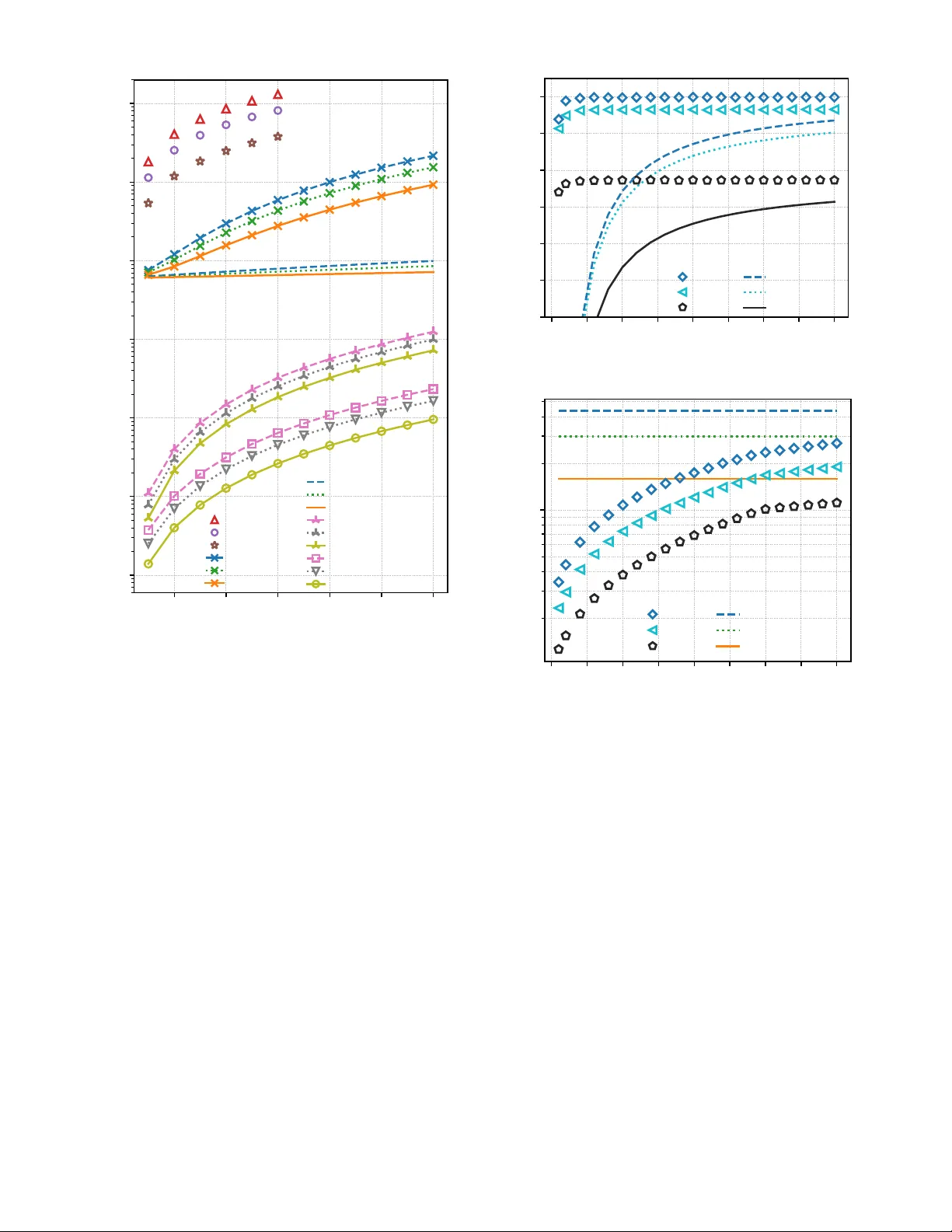
1 Joint Subcarrier and Po wer Allocation in NOMA: Optimal and Approximate Algorithms Lou Sala ¨ un, Student Member , IEEE , Marceau Coupechoux, and Chung Shue Chen, Senior Member , IEEE Abstract —Non-orthogonal multiple access (NOMA) is a promising technology to increase the spectral efﬁciency and enable massive connecti vity in 5G and future wir eless networks. In contrast to orthogonal schemes, such as OFDMA, NOMA multiplexes several users on the same frequency and time resour ce. Joint subcarrier and power allocation problems ( J S PA) in NOMA are NP-hard to solve in general. In this family of problems, we consider the weighted sum-rate (WSR) objective function as it can achieve various tradeoffs between sum-rate performance and user fairness. Because of JSP A ’ s intractability , a common approach in the literatur e is to solve separately the power control and subcarrier allocation (also known as user selection) problems, ther efor e achieving sub-optimal result. In this work, we ﬁrst improv e the computational complexity of existing single-carrier po wer contr ol and user selection schemes. These impro ved procedures are then used as basic building blocks to design new algorithms, namely O P T -J S PA, ε - J S PA and G R A D - J S PA. O P T - J S PA computes an optimal solution with lower complexity than current optimal schemes in the literature. It can be used as a benchmark for optimal WSR performance in simulations. Howev er , its pseudo-polynomial time complexity remains impractical for real-world systems with low latency requir ements. T o further reduce the complexity , we propose a fully polynomial-time approximation scheme called ε - J S PA. Since, no approximation has been studied in the literature, ε - J S PA stands out by allowing to control a tight trade-off between performance guarantee and complexity . Finally , G R A D - J S PA is a heuristic based on gradient descent. Numerical results show that it achieves near -optimal WSR with much lower complexity than existing optimal methods. I . I N T R O D U C T I O N In multi-carrier multiple access systems, the total frequency bandwidth is di vided into subcarriers and assigned to users to optimize the spectrum utilization. Orthogonal multiple access (OMA), such as orthogonal frequency-di vision multiple access (OFDMA) adopted in 3GPP-L TE and also 5G New Radio Phase 1 standards [1], [2], only serves one user per subcarrier in order to avoid intra-cell interference and hav e low-comple xity signal decoding at the receiv er side. OMA is known to be suboptimal in terms of spectral efﬁciency [3]. The principle of multi-carrier non-orthogonal multiple ac- cess (MC-NOMA) is to multiplex several users on the same subcarrier by performing signals superposition at the transmit- ter side. Successi ve interference cancellation (SIC) is applied at the recei ver side to mitigate interference between super - posed signals. MC-NOMA is a promising multiple access L. Sala ¨ un and C. S. Chen are with Bell Labs, Nokia Paris-Saclay , 91620 Nozay , France, and also with Lincs, Paris 75013, France (e-mail: lou.salaun@nokia-bell-labs.com; chung shue.chen@nokia-bell-labs.com). L. Sala ¨ un and M. Coupechoux are with L TCI, T elecom ParisT ech, Univ ersity of Paris-Saclay , Paris 75013, France (e-mail: marceau.coupechoux@telecom-paristech.fr). technology for 5G and beyond mobile networks as it can achiev e higher spectral efﬁcienc y than OMA schemes [4], [5]. Careful optimization of the transmit powers is required to control the intra-carrier interference of superposed signals and maximize the achiev able data rates. Besides, due to error propagation and decoding complexity concerns in practice [6], subcarrier allocation for each transmission also needs to be optimized. As a consequence, joint subcarrier and power allocation problems (JSP A) in NOMA ha ve recei ved much attention. In this class of problems, weighted sum-rate (WSR) maximization is especially important as it can achie ve dif ferent tradeoffs between sum-rate performance and user fairness [7]. T wo types of power constraints are considered in the lit- erature. On the one hand, cellular power constraint is mostly used in do wnlink transmissions to represent the total transmit power budget av ailable at the base station (BS). On the other hand, individual power constraint sets a power limit independently for each user . The latter is often considered in uplink scenarios [8], [9], nevertheless it can also be applied to the downlink [10], [11]. It is known that the equal-weight sum-rate and WSR max- imization are both strongly NP-hard if we consider individual power constraints in OFDMA [12] and in MC-NOMA sys- tems [11], [13]. Nev ertheless, sev eral algorithms have been dev eloped to perform subcarrier and/or po wer allocation for MC-NOMA and this type of constraints. Fractional transmit power control (FTPC) is a simple heuristic that allocates a fraction of the total power budget to each user based on their channel conditions [4]. In [8] and [9], heuristic user pairing strategies and iterativ e resource allocation algorithms are studied for uplink transmissions. A time efﬁcient two- step heuristic is introduced in [10] to solve the problem with equal weights. Reference [11] deriv es an upper bound on the optimal WSR and proposes a Lagrangian duality and dynamic programming (LDDP) scheme. This scheme achieves near- optimal result, assuming the power budget is divided in J equal parts to be allocated. It mainly serves as benchmark due to its high computational complexity when J is large in practical systems, which may not be suitable for low latenc y requirements. If we consider now cellular po wer constraints without individual power constraints, the equal-weight sum-rate max- imization is polynomial time solv able in OFDMA [14]. T o the best of our knowledge, it is unknown whether WSR maximization in MC-NOMA under this type of constraints is polynomial time solvable or NP-hard. Reference [15, Proposi- tion 1] prov es that the subcarrier optimization is NP-hard only in the case of equal power allocation among the users. The 2 proposed polynomial-time reduction from the NP-complete 3- dimensional matching (3DM) to the NOMA problem should hav e shown that all instances of 3DM can be mapped into an instance of the NOMA problem to be complete. Besides, the two-stage dynamic programming (TSDP) proposed in [11] solves it optimally in pseudo-polynomial time depending on J . Therefore, the WSR problem with cellular po wer constraint is weakly NP-hard at most (in contrast to str ongly NP-hard for the individual power constraints as mentioned pre viously). Only a few papers have developed optimization schemes in this setting, which are either heuristics with no theoretical performance guarantee or algorithms with impractical com- putational complexity . For example, a greedy user selection and heuristic po wer allocation scheme based on difference-of- con vex programming is proposed in [16]. In reference [15], a matching algorithm is dev eloped to perform subcarrier allocation. A minorization-maximization algorithm is used in [17] to compute precoding vectors of a MISO-NOMA system. The authors of [18] employ monotonic optimization to dev elop an optimal resource allocation policy , which serves as benchmark due to its exponential complexity . The TSDP scheme is also optimal for cellular power constraint scenarios as prov en in Theorem 13 of reference [11], but it has high pseudo-polynomial complexity as well. W e note that, to the best of our knowledge, no polynomial- time approximation scheme (PT AS) has been proposed in the literature. Although PT AS is interesting for practical consider- ations of NP-hard problems, as it provides theoretical perfor- mance guarantees with controllable computational complexity . Motiv ated by this observation, we e xtend the frame work of our previous paper [19] with a fully polynomial-time approxima- tion scheme (FPT AS) for the WSR maximization problem with cellular power constraint. In [19], we developed the following algorithms: two basic building blocks S C P C and S C U S which solve respecti vely the single-carrier po wer control and single- carrier user selection problems in polynomial time; and a heuristic JSP A scheme based on projected gradient descent, S C P C and S C U S , denoted here by G R A D - J S PA. Our contri- butions are as follo ws: 1) W e improve S C P C and S C U S by performing precom- putation to a void repeated operations each time they are ex ecuted. This reduces their computational complexity by a factor proportional to the number of users. 2) The above precomputation also speeds up G R A D - J S P A , which now has lo w and practical computational com- plexity . In addition, numerical results show that G R A D - J S PA achie ves near-optimal WSR, as well as signiﬁcant improv ement in performance over OMA. 3) W e develop a new optimal algorithm, called O P T - J S PA, suitable for use as a benchmark for optimal WSR per- formance in simulations. W e show that O P T - J S P A has lower computational comple xity than existing optimal schemes [11], [18]. 4) W e propose a FPT AS, which is denoted by ε - J S P A . Its design is based on the improv ed S C P C and S C U S , as well as techniques from the multiple choice knapsack prob- lem [20]. By deﬁnition of FPT AS, its performance is within a factor 1 − ε of the optimal, for any ε > 0 . Moreover , it has polynomial comple xity in both the input size and 1 / ε . Since, no approximation has been studied in the literature, ε - J S P A stands out by allowing to control a tight trade-of f between performance guarantee and complexity . Through the aforementioned points, our aim is to deepen the understanding of J S PA and NOMA resource allocation problems. W e de velop optimal, approximate and heuristic schemes which are each suitable for systems with different computational capabilities, as well as for performance bench- marking. In addition, we pro vide mathematical tools to study the WSR maximization problem, which can also be applied to other similar resource allocation problems. The paper is organized as follows. In Section II, we present the system model and notations. Section III formu- lates the WSR problem. W e consider two single-carrier sub- problems in Section IV that were previously solved using S C P C and S C U S in [19]. W e propose improved versions of these algorithms, namely i- S C P C and i-S C U S , which perform precomputation to reduce their complexity . Based on these basic building blocks, we dev elop a low complexity gradient descent based heuristic (G R A D - J S PA), a pseudo- polynomial time optimal algorithm ( O P T - J S PA) and a FPT AS with ε -approximation guarantee ( ε - J S P A ) in Section V. W e show in Section VI some numerical results, highlighting our solution’ s WSR performance and computational complexity . In Section VII, we discuss about ho w to generalize our framew ork to more realistic channel estimation models and multi-antenna systems. Finally , we conclude in Section VIII. I I . S Y S T E M M O D E L A N D N O TA T I O N S W e deﬁne in this section the system model and notations used throughout the paper . W e consider a downlink multi- carrier NOMA system composed of one base station (BS) serving K users. W e denote the index set of users by K , { 1 , . . . , K } , and the set of subcarriers by N , { 1 , . . . , N } . The total system bandwidth W is divided into N subcarriers of bandwidth W n , for each n ∈ N , such that P n ∈N W n = W . W e assume orthogonal frequency division, so that adjacent subcarriers do not interfere each other . Moreov er , each sub- carrier n ∈ N experiences frequency-ﬂat block fading on its bandwidth W n . Let p n k denotes the transmit power from the BS to user k ∈ K on subcarrier n ∈ N . User k is said to be activ e on subcarrier n if p n k > 0 , and inactiv e otherwise. In addition, let g n k be the channel gain between the BS and user k on subcarrier n , and η n k be the received noise power . W e assume that the channel gains are perfectly known. W e discuss about more realistic models with imperfect channel state information (CSI) in Section VII. For simplicity of notations, we deﬁne the normalized noise power as ˜ η n k , η n k /g n k . W e denote by p , ( p n k ) k ∈K ,n ∈N the vector of all transmit powers, and p n , ( p n k ) k ∈K the vector of transmit po wers on subcarrier n . In po wer domain NOMA, several users are multiple xed on the same subcarrier using superposition coding. A common approach adopted in the literature is to limit the number of superposed signals on each subcarrier to be no more than M . 3 The v alue of M is meant to characterize practical limitations of SIC due to decoding complexity and error propagation [6]. W e represent the set of active users on subcarrier n by U n , { k ∈ K : p n k > 0 } . The aforementioned constraint can then be formulated as ∀ n ∈ N , |U n | ≤ M , where |·| denotes the cardinality of a ﬁnite set. Each subcarrier is modeled as a multi-user Gaussian broadcast channel [6] and SIC is applied at the receiver side to mitigate intra-band interference. The SIC decoding order on subcarrier n is usually de- ﬁned as a permutation over the acti ve users on n , i.e., π n : { 1 , . . . , |U n |} → U n . Ho we ver , for ease of reading, we choose to represent it by a permutation over all users K , i.e., π n : { 1 , . . . , K } → K . These two deﬁnitions are equiv alent in our model since the Shannon capacity (2) does not depend on the inactiv e users k ∈ K \ U n , for which p n k = 0 . For i ∈ { 1 , . . . , K } , π n ( i ) returns the i -th decoded user’ s index. Con versely , user k ’ s decoding order is giv en by π − 1 n ( k ) . In this work, we consider the optimal decoding order studied in [6, Section 6.2]. It consists of decoding users’ signals from the highest to the lowest normalized noise po wer: ˜ η n π n (1) ≥ ˜ η n π n (2) ≥ · · · ≥ ˜ η n π n ( K ) . (1) User π n ( i ) ﬁrst decodes the signals of users π n (1) to π n ( i − 1) and subtracts them from the superposed signal before decoding its o wn signal. Interference from users π n ( j ) for j > i is treated as noise. The maximum achie vable data rate of user k on subcarrier n is giv en by Shannon capacity: R n k ( p n ) , W n log 2 1 + g n k p n k P K j = π − 1 n ( k )+1 g n k p n π n ( j ) + η n k ! , (a) = W n log 2 1 + p n k P K j = π − 1 n ( k )+1 p n π n ( j ) + ˜ η n k ! , (2) where equality (a) is obtained after normalizing by g n k . W e assume perfect SIC, therefore interference from users π n ( j ) for j < π − 1 n ( k ) is completely removed in (2). I I I . P R O B L E M F O R M U L A T I O N Let w = { w 1 , . . . , w K } be a sequence of K positive weights. The main focus of this work is to solve the following JSP A optimization problem: maximize p X k ∈K w k X n ∈N R n k ( p n ) , subject to C 1 : X k ∈K X n ∈N p n k ≤ P max , C 2 : X k ∈K p n k ≤ P n max , n ∈ N , C 3 : p n k ≥ 0 , k ∈ K , n ∈ N , C 4 : |U n | ≤ M , n ∈ N . ( P ) The objectiv e of P is to maximize the system’ s WSR. As discussed in Section I, this objectiv e function has receiv ed much attention since its weights w can be chosen to achiev e different tradeof fs between sum-rate performance and fair- ness [7]. Note that C 1 represents the cellular power constraint, i.e., a total power budget P max at the BS. In C 2 , we set a power limit of P n max for each subcarrier n . This is a common assumption in multi-carrier systems, e.g., [12], [14]. Constraint C 3 ensures that the allocated powers remain non-neg ati ve. Due to decoding complexity and error propagation in SIC [6], we restrict the maximum number of multiplex ed users per subcarrier to M in C 4 . For ease of reading, we summarize some system parameters of a given instance of P , for all n ∈ N , as follows: I n = ( w , K , W n , ( g n k ) k ∈K , ( η n k ) k ∈K ) . Let us consider the following change of v ariables: ∀ n ∈ N , x n i , ( P K j = i p n π n ( j ) , if i ∈ { 1 , . . . , K } , 0 , if i = K + 1 . (3) W e deﬁne x , ( x n i ) i ∈{ 1 ,...,K } ,n ∈N and x n , ( x n i ) i ∈{ 1 ,...,K } . Lemma 1 (Equiv alent problem P 0 ) . Pr oblem P is equivalent to pr oblem P 0 formulated below: maximize x X n ∈N K X i =1 f n i ( x n i ) + A, ( P 0 ) subject to C 1 0 : X n ∈N x n 1 ≤ P max , C 2 0 : x n 1 ≤ P n max , n ∈ N , C 3 0 : x n i ≥ x n i +1 , i ∈ { 1 , . . . , K } , n ∈ N , C 3 00 : x n K +1 = 0 , n ∈ N , C 4 0 : |U 0 n | ≤ M , n ∈ N , wher e for any i ∈ { 1 , . . . , K } and n ∈ N , we have: f n i ( x n i ) ,      W n log 2  x n 1 + ˜ η n π n (1)  w π n (1)  , if i = 1 , W n log 2  ( x n i + ˜ η n π n ( i ) ) w π n ( i )  x n i + ˜ η n π n ( i − 1)  w π n ( i − 1)  , if i > 1 , and where U 0 n , { i ∈ { 1 , . . . , K } : x n i > x n i +1 } . The constant term A = P n ∈N w π n ( K ) log 2  1 / ˜ η n π n ( K )  is chosen so that P and P 0 have e xactly the same optimal value. Pr oof: The idea is to apply the change of variables (3) to problem P . Details of the calculation can be found in Appendix A. The adv antage of this formulation P 0 is that it e xhibits a sep- arable objectiv e function in both dimensions i ∈ { 1 , . . . , K } and n ∈ N . In other words, it can be written as a sum of functions f n i , each only depending on one v ariable x n i . I V . S I N G L E - C A R R I E R O P T I M I Z A T I O N In this section, we focus on a simpler problem, in which there is a single subcarrier n ∈ N and a power budget ¯ P n is giv en for this subcarrier: F n  ¯ P n  = max x n K X i =1 f n i ( x n i ) + A n , ( P 0 S C ( n ) ) subject to C 2 0 – 3 0 : ¯ P n ≥ x n 1 ≥ . . . ≥ x n K ≥ 0 , C 4 0 : |U 0 n | ≤ M , 4 where A n = w π n ( K ) log 2  1 / ˜ η n π n ( K )  . C 2 0 – 3 0 is obtained by combining C 2 0 , C 3 0 and C 3 00 . F n  ¯ P n  denotes its optimal value. Algorithms S C P C and S C U S have been introduced in our previous paper [19] to tackle respectiv ely the single- carrier po wer control and single-carrier user selection sub- problems that arise from P 0 S C ( n ) . W e provide technical details of these algorithms belo w , and we show how precomputation can further improv e their computational complexity . They will be used as basic building blocks in Section V to design efﬁcient algorithms G R A D - J S PA, O P T - J S P A and ε - J S P A, for the joint resource allocation problem. A. Analysis of the Separ able Functions f n i W e introduce auxiliary functions to help us in the analysis of f n i and the algorithm design. For n ∈ N , i ∈ { 1 , . . . , K } and j ≤ i , assume that the consecutiv e variables x n j , . . . , x n i are all equal to a certain value x ∈  0 , ¯ P n  . W e deﬁne f n j,i as: f n j,i ( x ) , i X l = j f n l ( x ) , =      W n log 2  x + ˜ η n π n ( i )  w π n ( i )  , if j = 1 , W n log 2  ( x + ˜ η n π n ( i ) ) w π n ( i )  x + ˜ η n π n ( j − 1)  w π n ( j − 1)  , if j > 1 . This simpliﬁcation of notation is relev ant for the analysis of S C P C and S C U S in the following subsections. Indeed, if users j, . . . , i − 1 are not activ e (i.e., j, . . . , i − 1 / ∈ U 0 n ), then x n j = · · · = x n i , therefore P i l = j f n l can be replaced by f n j,i and x n j +1 , . . . , x n i are redundant with x n j . If constraint C 4 0 is satisﬁed, up to M users are activ e on each subcarrier . Thus, ev aluating the objective function of P 0 S C ( n ) only requires O ( M ) operations. W e study the properties of f n j,i in Lemma 2. Note that f n i = f n i,i , therefore Lemma 2 also holds for functions f n i . Fig. 1 shows the two general forms that can be taken by f n j,i . Lemma 2 (Properties of f n j,i ) . Let n ∈ N , i ∈ { 1 , . . . , K } , and j ≤ i , we have: • If j = 1 or w π n ( i ) ≥ w π n ( j − 1) , then f n j,i is incr easing and concave on [0 , ∞ ) . • Otherwise when j > 1 and w π n ( i ) < w π n ( j − 1) , f n j,i is unimodal. It incr eases on  − ˜ η π n ( j − 1) , c 1  and decr eases on [ c 1 , ∞ ) , wher e c 1 = w π n ( j − 1) ˜ η π n ( i ) − w π n ( i ) ˜ η π n ( j − 1) w π n ( i ) − w π n ( j − 1) . Besides, f n j,i is concave on  − ˜ η π n ( j − 1) , c 2  and conve x on [ c 2 , ∞ ) , wher e c 2 = √ w π n ( j − 1) ˜ η π n ( i ) − √ w π n ( i ) ˜ η π n ( j − 1) √ w π n ( i ) − √ w π n ( j − 1) ≥ c 1 . Pr oof: These analytical properties can be obtained by studying the ﬁrst and second deriv ativ es of f n j,i . Details can be found in Appendix B. W e present in Algorithm 1 the pseudocode A R G M A X f which computes the maximum of f n j,i on  0 , ¯ P n  following the result of Lemma 2. A R G M A X f only requires a constant number of basic operations, therefore its comple xity is O (1) . max at c 1 change of conve xity at c 2 f n j , i , for w π n ( i ) < w π n ( j − 1) f n j , i , for w π n ( i ) ≥ w π n ( j − 1) Fig. 1. The two general forms of functions f n j,i Algorithm 1 Compute maximum of f n j,i on  0 , ¯ P n  function A R G M A X f  j, i, I n , ¯ P n  1: a ← π n ( i ) 2: b ← π n ( j − 1) 3: if j = 1 or w a ≥ w b then 4: retur n ¯ P n 5: else 6: retur n max n 0 , min n w b ˜ η a − w a ˜ η b w a − w b , ¯ P n oo 7: end if end function B. Single-Carrier P ower Contr ol The single-carrier po wer control problem P 0 S C P C ( n ) is equiv alent to problem P 0 S C ( n ) , with the exception that a ﬁxed user selection U 0 n (or equiv alently U n ) is giv en as input instead of being an optimization variable. It is deﬁned below: maximize x n K X i =1 f n i ( x n i ) + A n , ( P 0 S C P C ( n ) ) subject to C 2 0 – 3 0 : ¯ P n ≥ x n 1 ≥ . . . ≥ x n K ≥ 0 . W e denote its optimal value by F n  U 0 n , ¯ P n  . Since inacti ve users k / ∈ U n hav e no contribution on the data rates, i.e., p n k = 0 and R n k = 0 , we remove them for the study of this sub-problem. W ithout loss of generality , we inde x the remaining activ e users on subcarrier n by i n ∈ { 1 n , . . . , |U 0 n | n } . For example, if U 0 n = { 4 , 7 , 10 } , then 1 n = 4 , 2 n = 7 and 3 n = 10 . For simplicity of notation, we add an index 0 n = 0 , which does not correspond to any user . From the deﬁnition of U 0 n , variables x n l with index from l = ( i − 1) n + 1 to i n are equal, for any i ≥ 1 . In the above example, we would hav e x 1 = x 2 = x 3 = x 4 > x 5 = x 6 = x 7 > x 8 = x 9 = x 10 . Thus, the objectiv e function of P 0 S C P C ( n ) can be written as: K X i =1 f n i ( x n i ) + A n = |U 0 n | X i =1 f n ( i − 1) n +1 ,i n  x n i n  + B n , (4) where B n = A n if the last acti ve user’ s index is |U 0 n | n = K , and B n = f n |U 0 n | n +1 ,K (0) + A n otherwise. For 1 ≤ j ≤ i ≤ K , we simplify some notations as follo ws: ˜ f n j,i ( U 0 n , · ) , f n ( j − 1) n +1 ,i n ( · ) , A R G M A X ˜ f  j, i, I n , U 0 n , ¯ P n  , A R G M A X f  ( j − 1) n + 1 , i n , I n , ¯ P n  . 5 W e reformulate the problem as: maximize x n i n |U 0 n | X i =1 ˜ f n i,i  U 0 n , x n i n  + B n , ( P 0 S C P C ( n ) ) subject to C 2 0 – 3 0 : ¯ P n ≥ x n 1 n ≥ . . . ≥ x n |U 0 n | n ≥ 0 . Algorithm 2 presents the S C P C method proposed in [19]. The idea is to iterate over variables x n i n for i = 1 to |U 0 n | , and com- pute their optimal v alue x ∗ = A R G M A X ˜ f ( i, i, I n , U 0 n , ¯ P n ) at line 3. If the current allocation satisﬁes constraint C 3 0 , then x n i n gets value x ∗ . Otherwise, the algorithm backtracks at line 6 and ﬁnds the highest index j ∈ { 1 , . . . , i − 2 } such that x n j n ≥ A R G M A X ˜ f ( j + 1 , i, I n , U 0 n , ¯ P n ) . Then, variables x n ( j +1) n , . . . , x n i n are set equal to A R G M A X ˜ f ( j + 1 , i, I n , U 0 n , ¯ P n ) at line 10. The optimality and complexity of S C P C are presented in Theorem 3. Algorithm 2 Single-carrier po wer control algorithm ( S C P C ) function S C P C  I n , U 0 n , ¯ P n  1: for i = 1 to |U 0 n | do 2:  Compute the optimal of ˜ f n i,i 3: x ∗ ← A R G M A X ˜ f  i, i, I n , U 0 n , ¯ P n  4:  Modify x ∗ if this allocation violates constraint C 3 0 5: j ← i − 1 6: while x n j n < x ∗ and j ≥ 1 do 7: x ∗ ← A R G M A X ˜ f  j, i, I n , U 0 n , ¯ P n  8: j ← j − 1 9: end while 10: x n ( j +1) n , . . . , x n i n ← x ∗ 11: end for 12: return x n 1 n , . . . , x n |U 0 n | n end function Theorem 3 (Optimality and complexity of S C P C ) . Given subcarrier n ∈ N , a set U 0 n of M active users and a power budg et ¯ P n , algorithm S C P C computes the optimal single-carrier power contr ol. Its worst case computational complexity is O  M 2  . Pr oof: W e prove this theorem in Appendix C by mathe- matical induction combined with Lemma 2. In multi-carrier resource allocation schemes, such as G R A D - J S PA and ε - J S P A, it is often required to compute the optimal single-carrier power control and WSR for man y different values of power budget ¯ P n . In these cases, running many times S C P C is actually not efﬁcient in terms of computational complexity , since se veral computations may be repeated. T o av oid this, we propose in Algorithm 3 an improv ed S C P C algorithm (i- S C P C ). The idea is to perform precomputation before runtime by calling S C P C ( I n , U 0 n , P max ) and storing its result x n 1 n , . . . , x n |U 0 n | n as a global variable (also called lookup table). Any subsequent ev aluation with input I n , U 0 n , ¯ P n , where ¯ P n ≤ P max , can be obtained as in line 1. Theorem 4 (Optimality and complexity of i- S C P C ) . Given subcarrier n ∈ N and a set U 0 n of M active users, the pr ecomputation of i- S C P C has complexity O  M 2  . Any subsequent e valuation costs O ( M ) . Hence, for C differ ent Algorithm 3 Improved S C P C algorithm with precomputation input: I n , U 0 n , P max global variable: x n 1 n , . . . , x n |U 0 n | n initialization: x n 1 n , . . . , x n |U 0 n | n ← S C P C ( I n , U 0 n , P max ) function i- S C P C  ¯ P n  1: return min { x n 1 n , ¯ P n } , . . . , min { x n |U 0 n | n , ¯ P n } end function power budg ets, algorithm i- S C P C computes their respective optimal single-carrier power contr ol with overall complexity O  M 2 + C M  . Pr oof: W e show in Appendix D that subsequent ev alua- tions of S C P C can be obtained as in line 1 of Algorithm 3. Remark. Note that S C P C and i- S C P C r eturns |U 0 n | values x n 1 n , . . . , x n |U 0 n | n r epresenting only the active users’ variables. These values are sufﬁcient to compute the optimal power allocation and WSR of P 0 S C P C ( n ) as shown in Eqn. (4). If needed, the full vector x n can be obtained by the following pr ocedure in O ( K ) operations: 1: for i = 1 to |U 0 n | and l = ( i − 1) n + 1 to i n do 2: x n l ← x n i n 3: end for 4: for l = |U 0 n | n + 1 to K do 5: x n l ← 0 6: end for C. Single-Carrier User Selection Unlike in the pre vious subsection, we consider here further- more the user selection U 0 n optimization under multiplexing and SIC constraint C 4 0 , i.e., we solve P 0 S C ( n ) . In [19], a dynamic programming (DP) is proposed to solve P 0 S C ( n ) . Here, we ﬁrst dev elop a similar DP procedure in Algorithm 4 (S C U S ). Then, we propose an improv ed version (i-S C U S ) which performs S C U S as precomputation. The idea of S C U S is to compute recursi vely the elements of three arrays V , X , U . Let m ∈ { 0 , . . . , M } , j ∈ { 1 , . . . , K } and i ∈ { j, . . . , K } , we deﬁne V [ m, j, i ] as the optimal value of the following problem P 0 S C [ m, j, i ] : V [ m, j, i ] , max x n K X l = j f n l ( x n l ) , ( P 0 S C [ m, j, i ] ) subject to C 2 0 , C 3 0 , C 3 00 , C 4 0 : |U 0 n | ≤ m, C 5 0 : x n j = · · · = x n i . This problem is more restrictiv e than P 0 S C ( n ) . The objectiv e function only depends on variables x n j , . . . , x n K . C 4 0 limits the number of acti ve users to m . Moreov er , variables x n j , . . . , x n i are equal according to C 5 0 . It is interesting to note that V [ M , 1 , 1] is the optimal v alue of P 0 S C ( n ) , since the objective function is P K l =1 f n l ( x n l ) for j = 1 and constraint C 5 0 becomes tri vially true for j = i . Let x n j ∗ , . . . , x n K ∗ be the optimal solution achieving V [ m, j, i ] . W e deﬁne X [ m, j, i ] , x n i ∗ , which is also equal to x n j ∗ , . . . , x n i − 1 ∗ 6 Algorithm 4 Single-carrier user selection algorithm ( S C U S) function S C U S  I n , M , ¯ P n  1:  Initialize arrays V , X , U for m = 0 and i = K 2: for i = K to 1 and j = i to 1 do 3: V [0 , j, i ] ← f n j,K (0) 4: X [0 , j, i ] ← 0 5: U [0 , j, i ] ← ∅ 6: end for 7: for m = 1 to M and j = K to 1 do 8: x ∗ ← A R G M A X f  j, K, I n , ¯ P n  9: V [ m, j, K ] ← f n j,K ( x ∗ ) 10: X [ m, j, K ] ← x ∗ 11: U [ m, j, K ] ← ∅ 12: end for 13:  Compute V , X , U for m ∈ [1 , M ] and j ≤ i ≤ K − 1 14: for i = K − 1 to 1 and m = 1 to M and j = i to 1 do 15: x ∗ ← A R G M A X f  j, i, I n , ¯ P n  16: v act ← f n j,i ( x ∗ ) + V [ m − 1 , i + 1 , i + 1] 17: v inact ← V [ m, j, i + 1] 18: if v act > v inact and x ∗ > X [ m − 1 , i + 1 , i + 1] then 19: V [ m, j, i ] ← v act 20: X [ m, j, i ] ← x ∗ 21: U [ m, j, i ] ← ( m − 1 , i + 1 , i + 1) 22: else 23: V [ m, j, i ] ← v inact 24: X [ m, j, i ] ← X [ m, j, i + 1] 25: U [ m, j, i ] ← ( m, j, i + 1) 26: end if 27: end for 28:  Retriev e the optimal solution x n 29: x n 1 , . . . , x n K ← 0 30: ( m, j, i ) ← ( M , 1 , 1) 31: repeat 32: x n j , . . . , x n i ← X [ m, j, i ] 33: ( m, j, i ) ← U [ m, j, i ] 34: until ( m, j, i ) = ∅ 35: return x n end function due to constraint C 5 0 . The idea of SCUS is to recursi vely compute the elements of V through the following relation: V [ m, j, i ] =      v act , if v act > v inact and x ∗ > X [ m − 1 , i + 1 , i + 1] , v inact , otherwise , (5) where x ∗ = A R G M A X f  j, i, I n , ¯ P n  , and v act (resp. v inact ) corresponds to allocation where user i is active (resp. inacti ve): v act = f n j,i ( x ∗ ) + V [ m − 1 , i + 1 , i + 1] , v inact = V [ m, j, i + 1] . During SCUS’ s iterations, the array U keeps track of which previous element of V has been used to compute the current value function V [ m, j, i ] . This allows us to retrieve the entire optimal vector x n at the end of Algorithm 4 (at lines 28- 35) by backtracking from index ( M , 1 , 1) to ∅ , where ∅ is set at initial indices (see lines 5 and 11) to indicate the recursion termination. T o sum up, X and U have two dif ferent recurrence relations depending on the cases in Eqn. (5). If V [ m, j, i ] = v act , then: X [ m, j, i ] = x ∗ , U [ m, j, i ] = ( m − 1 , i + 1 , i + 1) . If V [ m, j, i ] = v inact , then: X [ m, j, i ] = X [ m, j, i + 1] , U [ m, j, i ] = ( m, j, i + 1) . When m = 0 , no user can be active on this subcarrier due to constraint C 4 0 . Therefore, V , X , U can be initialized by: V [0 , j, i ] = f n j,K (0) , X [0 , j, i ] = 0 , U [0 , j, i ] = ∅ . For simplicity , we also extend V , X and U on the index i = K and j ≤ K and initialize them as follows: V [ m, j, K ] = f n j,K ( x ∗ ) , X [ m, j, K ] = x ∗ , U [ m, j, K ] = ∅ . A detailed analysis is giv en in Appendix E. Theorem 5 (Optimality and complexity of S C U S ) . Given a subcarrier n ∈ N , a power budget ¯ P n and M ≥ 1 , algorithm S C U S computes the optimal single-carrier power contr ol and user selection of P 0 S C ( n ) . Its worst case compu- tational comple xity is O  M K 2  . Pr oof: The proof is done by induction based on the principle of dynamic programming. See Appendix E. W e present i- S C U S in Algorithm 5, which performs pre- computation to avoid repeating the DP procedure when mul- tiple ev aluations are required. The algorithm precomputes vectors V , X , U from S C U S ( I n , M , P max ) before runtime, at line 1. Then, in lines 2-5, it retrie ves the activ e users set U 0 n and optimal solution x n 1 , . . . , x n K of each V [ M , 1 , i ] , i ∈ { 1 , . . . , K } , and stores them in col lection . Any subsequent ev aluation with a lower b udget ¯ P n ≤ P max , can be obtained by searching the best allocation among the K possibilities in col l ection (lines 6-7). Each allocation is truncated as in i-S C P C  ¯ P n  to satisfy b udget ¯ P n . The optimality and complexity of Algorithm 5 are given in Theorem 6. Theorem 6 (Optimality and complexity of i- S C U S ) . Given a subcarrier n ∈ N , a power budget ¯ P n and M ≥ 1 , the precomputation of i- S C U S has complexity O  M K 2  . Any subsequent evaluation costs O ( M K ) . Hence, for C differ ent power budg ets, i- S C U S computes their r espective optimal single-carrier power contr ol and user selection P 0 S C ( n ) with overall complexity O  M K 2 + C M K  . Pr oof: See Appendix F. T able I summarizes the complexity of the single-carrier algorithms dev eloped in this section. They will be used as basic b uilding blocks to design JSP A schemes in Section V. 7 Algorithm 5 Improved S C U S algorithm with precomputation input: I n , M , P max global variable: col l ection initialization: 1: Get V , X , U from S C U S ( I n , M , P max ) 2: for i = 1 to K do 3: Retriev e the activ e users set U 0 n of V [ M , 1 , i ] and its optimal solution x n 1 , . . . , x n K 4: Add ( U 0 n , x n 1 , . . . , x n K ) to col l ection 5: end for function i- S C U S  ¯ P n  6: Get ( U 0 n , x n 1 , . . . , x n K ) in coll ection that maximizes F n ( U 0 n , ¯ P n ) = P |U 0 n | l =1 ˜ f n l,l  U 0 n , min { x n l n , ¯ P n }  + B n 7: return min { x n 1 , ¯ P n } , . . . , min { x n K , ¯ P n } end function T ABLE I S U M M A RY O F T H E S I N G L E - C A R R I E R R E S O U R C E A L L O C ATI O N S C H E M E S Algorithm Complexity to perform C ev aluations S C P C [19] O  C M 2  i-S C P C O  M 2 + C M  S C U S [19] O  C M K 2  i-S C U S O  M K 2 + C M K  V . J O I N T S U B C A R R I E R A N D P O W E R A L L O C A T I O N Recall that F n  ¯ P n  is the optimal value of P 0 S C ( n ) with power b udget ¯ P n . W e have F n  ¯ P n  = P K i =1 f n i ( x n i ) + A n , where x n 1 , . . . , x n K is the output of i- S C U S  ¯ P n  . Using this notation, the JSP A problem P 0 can be simpliﬁed as: maximize ¯ P X n ∈N F n  ¯ P n  , ( P 0 M C ) subject to ¯ P n ∈ F , where ¯ P n , for n ∈ N , are intermediate variables representing each subcarrier’ s power budget. ¯ P ,  ¯ P 1 , . . . , ¯ P N  denotes the po wer budget vector . The feasible set F , { ¯ P : X n ∈N ¯ P n ≤ P max and 0 ≤ ¯ P n ≤ P n max , n ∈ N } is chosen to satisfy C 1 0 and C 2 0 in P 0 . Problem P 0 M C consists in optimizing the power budget ¯ P n allocated to each subcarrier n . For a giv en b udget ¯ P n , F n  ¯ P n  is computed by ﬁnding the optimal single-carrier user selection and power control using i- S C U S  ¯ P n  . The choice of ¯ P n affects the single-carrier user selection and po wer control, i.e., v ariables x n and U 0 n . The latter inﬂuence the value of F n , which in turn has an impact on the power budget optimization. Although variables x n and U 0 n are hidden in F n , they are nev ertheless optimized jointly with ¯ P n . Indeed, we can see that P 0 M C is equiv alent to P 0 when replacing F n by its deﬁnition in P 0 S C ( n ) along with its constraints C 2 0 to C 4 0 . A. Gradient Descent Based Heuristic G R A D - J S P A is an efﬁcient heuristic based on projected gradient descent. Its principle is to perform a two-stage opti- mization as presented in Fig. 2. The ﬁrst-stage is a projected gradient descent on ¯ P in the search space F . The gradient descent requires to ev aluate P n ∈N F n and its gradient at each iteration. This task is carried out by i- S C U S in the second- stage. W e denote the deriv ativ e of F n at ¯ P n by F n 0  ¯ P n  . Lemma 7 shows how to compute it. As illustrated in Fig. 2, the second-stage is called at each gradient iteration to return F n  ¯ P n  and F n 0  ¯ P n  to the ﬁrst-stage, for all n ∈ N . Lemma 7 (Deriv ative of F n ) . Let x n 1 , . . . , x n K be the output of i- S C U S  ¯ P n  . The left deriva- tive of F n at ¯ P n , can be computed as follows: F n 0  ¯ P n  = W n w π n ( l )  x n l + ˜ η n π n ( l )  ln(2) = W n w π n ( l )  ¯ P n + ˜ η n π n ( l )  ln(2) , wher e l is the gr eatest index such that x n l = ¯ P n , and ln(2) is the natural logarithm of 2 . Pr oof: T o get F n 0 , we ﬁrst prove that F n 0  U 0 n , ¯ P n  = f n 0 1 ,l  ¯ P n  and F n ( ¯ P n ) = max U 0 n { F n ( U 0 n , ¯ P n ) } , where max is taken o ver all activ e users sets in col l ection of i-S C U S . See Appendix G for the detailed proof of semi-differentiability . First-stage algorithm: projected gradient descent Follo w the gradient of P n ∈N F n ( ¯ P n ) and up date each sub carrier’s pow er budget ¯ P n in the simplex F Second-stage algorithm: i- SCUS Compute the optimal single-carrier p ow er allo cation x n under budget ¯ P n and constraint |U 0 n | ≤ M Input: M , P max , P n max in out Output: optimal p ow er allocation among sub carriers ¯ P Fo r each F n evaluation: I n , M , ¯ P n in out F n ( ¯ P n ) , F n 0 ( ¯ P n ) Fig. 2. Overvie w of G R A D - J S P A The pseudocode of G R A D - J S P A is described in Algo- rithm 6. Input ξ corresponds to the error tolerance at ter- mination, as we can see at line 8. The search direction at lines 4-5 is the gradient of P n ∈N F n ev aluated at ¯ P . Since F 1 , . . . , F N are independent, it is equal to the vector of F 1 0  ¯ P 1  , . . . , F N 0  ¯ P N  . Note that the step size α at line 6 can be tuned by backtracking line search or exact line search [21, Section 9.2]. W e adopt the latter to perform simulations. The projection of ¯ P + α ∆ on the simplex F at line 7 can be computed efﬁciently [21, Section 8.1.1], the details of its implementation are omitted here. W e showed in our pre vious work [19] that G R A D - J S PA worst case complexity is O  log(1 /ξ ) N M K 2  when S C U S is used to ev aluate functions F n , n ∈ N . W e show in Theorem 8 that the complexity of G R A D - J S P A can be reduced by the use of i-S C U S . Theorem 8 (Complexity of G R A D - J S P A) . Let ξ be the err or tolerance at termination. Algorithm G R A D - J S PA has complexity O  N M K 2 + log(1 /ξ ) N M K  when i- S C U S is used to evaluate functions F n , n ∈ N . Pr oof: In Appendix G, we prove that the objectiv e function is piece-wise α -strongly concave and β -smooth. 8 Algorithm 6 Gradient descent based heuristic ( G R A D - J S PA) function G R A D - J S P A  ( I n ) n ∈N , M , P max , P n max , ξ  1: Let ¯ P ← 0 be the starting point 2: repeat 3: Sav e the previous vector ¯ P 0 ← ¯ P 4: Determine a search direction ∆ 5: ∆ ←  F 1 0  ¯ P 1  , . . . , F N 0  ¯ P N  6: Choose a step size α 7: Update ¯ P ← projection of ¯ P + α ∆ on F 8: until || ¯ P 0 − ¯ P || ≤ ξ 9: return ¯ P end function Therefore, the con ver gence to a local optimum follows from classical con vex optimization results [22, Section 2.2.4]. Although i- S C U S (or equiv alently S C U S ) is optimal, the returned F n  ¯ P n  is not necessarily concave in ¯ P n . As a consequence, G R A D - J S PA is not guaranteed to con verge to a global maximum. Nev ertheless, we show by numerical results in Section VI that it achie ves near-optimal WSR performance with lo w complexity . B. Pseudo-P olynomial T ime Optimal Scheme The JSP A problem as formulated in P 0 M C has real variables ¯ P n on a continuous search space F . Ho wever , the study of NP- hard optimization problems and their approximation requires parameters and variables to be represented by a bounded number of bits [23], i.e., with bounded precision. This is also a reasonable assumption in practice since MC-NOMA systems are subject to minimum transmit power limitation at the BS and ﬂoating-point arithmetic precision of the hardware. As a consequence, we discretize the search space F , in the same way as in [11]. Let δ be the minimum transmit power such that the v ariables ¯ P n can only take value of the form l · δ , for l ∈ { 0 , 1 , . . . , b P max δ c} . W e denote the number of non-zero power values as J = b P max δ c . The feasible set then becomes F 0 , { ¯ P : X n ∈N ¯ P n ≤ P max and 0 ≤ ¯ P n ≤ P n max , n ∈ N , and ¯ P n = l · δ, l ∈ { 0 , . . . , J } , n ∈ N } . W e re write problem P 0 M C with search space F 0 as follo ws: maximize y X n ∈N J X l =1 c n,l y n,l , (MCKP) subject to X n ∈N J X l =1 a n,l y n,l ≤ P max , J X l =1 a n,l y n,l ≤ P n max , n ∈ N , J X l =1 y n,l ≤ 1 , n ∈ N , y n,l ∈ { 0 , 1 } , n ∈ N , l ∈ [1 , J ] , where c n,l = F n ( l · δ ) and a n,l = l · δ . The discretized JSP A problem, denoted by MCKP, is known as the multiple choice knapsack problem [20]. It has N disjoint classes each containing J items to be packed into a knapsack of capacity P max . Each item has a proﬁt c n,l and a weight a n,l , representing respectively the WSR and power consumption of this allocation on subcarrier n . The binary variable y n,l takes value 1 if and only if item l in class n is assigned to the knapsack. The problem consists in assigning at most one item from each class to maximize the sum of their proﬁt. W e denote its optimal value by F ∗ M C K P . As mentioned previously , discretizing P 0 M C is necessary due to the bounded precision which arises inherently from the study of algorithms and their implementation in practical sys- tems. Besides, MCKP can be used to approach the continuous solution of P 0 M C with arbitrary precision. Indeed, Theorem 9 shows that the discretization error is upper -bounded by a linear function in δ with a coefﬁcient depending on the system’ s parameters. Theorem 9 (Discretization error between F ∗ and F ∗ M C K P ) . The gap between the optimal values of the continuous pr ob- lem P 0 M C and its discr etized version MCKP with step size δ is upper -bounded by: F ∗ − F ∗ M C K P ≤ δ X n ∈N max k ∈K ( W n w π n ( k )  ¯ P n ∗ + ˜ η n π n ( k )  ln(2) ) , wher e ¯ P n ∗ is the optimal power budget of P 0 M C on subcarrier n ∈ N . Pr oof: W e deriv e the proof in Appendix H. The discrete problem MCKP can be solved optimally by dy- namic pr ogramming by weights studied in [20, Section 11.5]. Based on this idea, we propose O P T - J S P A (see Algorithm 7) to solve P 0 M C . W e ﬁrst transform P 0 M C to problem MCKP: from line 1 to 5, e very item’ s proﬁt c n,l is computed using i- S C U S . Then, we perform dynamic programming by weights at lines 6-7. W e summarize the optimality and comple xity of O P T - J S P A in Theorem 10. Detailed analysis of the dynamic programming can be found in Appendix I. Algorithm 7 The pseudo-polynomial time optimal scheme function O P T - J S P A  ( I n ) n ∈N , M , P max , P n max , δ  1:  Compute the parameters of MCKP 2: for n ∈ N and l ∈ [0 , J ] do 3: a n,l ← l · δ 4: c n,l ← F n ( l · δ ) 5: end for 6: return optimal allocation from the dynamic pr ogr am- 7: ming by weights [20] end function Theorem 10 (Optimality and complexity of O P T - J S P A) . Given a minimum transmit power δ , algorithm O P T - J S P A computes the optimal of P 0 M C on the discr ete set F 0 . Its computational complexity is O  N M K 2 + J N M K + J 2 N  , which is pseudo-polynomial in J . Pr oof: W e explain the principle of dynamic programming by weights and deriv e its complexity in Appendix I. 9 T ABLE II C O M PA R I S O N O F S O M E J S P A S C H E M E S P R O P O S E D I N T H I S W O R K A N D I N T H E L I T E R ATU R E Algorithm Perf ormance guarantee Complexity for J discrete power values Monotonic optimization with outer polyblock approximation [18] Optimal Exponential in K and N T S D P [11] Optimal O  J 2 N M K  O P T - J S PA Optimal O  N M K 2 + J N M K + J 2 N  ε - J S PA FPT AS, i.e., its performance is within a factor 1 − ε of the optimal, for any ε > 0 O  N M K 2 + min n log( J ) N 2 M K ε + N 3 ε 2 , J N M K + J 2 N o G R A D - J S PA Heuristic O  N M K 2 + log ( J ) N M K  O P T - J S P A is said to be pseudo-polynomial since it depends on the total number of power values J , whereas all system’ s parameters and variables are encoded in O (log ( J )) bits. As a consequence, in practical systems, the contribution of J to the computation time is way higher than parameters N , K , M . C. Fully P olynomial-T ime Appr oximation Scheme W e de velop a FPT AS to av oid the pseudo-polynomial com- plexity in J that is inherent to the optimal schemes O P T - J S PA and T S D P [11]. According to [24], an algorithm is said to be a FPT AS if it outputs a solution within a factor 1 − ε of the optimal, for any ε > 0 . Moreover , its running time is bounded by a polynomial in both the input size and 1 / ε . A FPT AS is the best trade-off one can hope for an NP-hard optimization problem in terms of performance guarantee and complexity , assuming P 6 = NP . The proposed FPT AS, called ε - J S P A (see Algorithm 8), is based on dynamic programming with scaled proﬁts. Scaling the proﬁts is a common technique to reduce the number of items computed in MCKP. First, we compute an estimation U of MCKP’ s optimal value, such that U ≥ F ∗ M C K P ≥ U / 4 . W e explain the estimation procedure in Appendix J. Then, instead of computing all J N proﬁt values c n,l , we only consider the subset L n of items on each subcarrier n such that: L n , { l 0 ≤ J, l ≤ 4 N ε − 1 : c n,l 0 ≥ l ε U 4 N > c n,l 0 − 1 } . This can be seen as considering only one proﬁt value per interval of the form [( l − 1) · ε U / 4 N , l · ε U / 4 N ] , for l ∈ { 1 , . . . , 4 N/ ε } . Each L n , for n ∈ N , can be obtained by multi-key binary search [25]. All function ev aluations required by the multi-key binary search are done by i- S C U S . Finally , we apply the dynamic pr ogramming by pr oﬁts [20, Section 11.5] in lines 5-6. It is known that the optimal solution obtained by dynamic programming by proﬁts considering only items in L n , dif fers from F ∗ M C K P by at most a factor 1 − ε . The performance of ε - J S P A are summarized in Theorem 11. W e provide more details on the estimation U in Appendix J and the dynamic programming by proﬁts in Appendix K. Theorem 11 (Performance and complexity of ε - J S PA) . Given a minimum transmit power δ and an appr oximation factor ε , algorithm ε - J S P A computes an ε -appr oximation of P 0 M C on the discrete set F 0 . The algorithm is a FPT AS with asymptotic complexity: O  N M K 2 + min n log( J ) N 2 M K ε + N 3 ε 2 , J N M K + J 2 N o . Pr oof: W e deriv e this result in Appendix K, using the dynamic programming by proﬁts and the estimation procedure studied in Appendix J. Algorithm 8 The proposed FPT AS ( ε - J S PA) function ε - J S P A  ( I n ) n ∈N , M , P max , P n max , δ, ε  1: Compute an estimation U of F ∗ M C K P 2: for n ∈ N do 3: Get a n,l , c n,l , for l ∈ L n by multi-ke y binary search 4: end for 5: return ε -approximate allocation from the dynamic 6: pr ogramming by pr oﬁts [20] end function D. Comparison of JSP A Algorithms In T able II, we compare the performance and complexity of the proposed algorithms with JSP A schemes in the literature. Reference [18] studied an optimal monotonic optimization framew ork, which has exponential complexity in K and N . The two-stage dynamic programming algorithm (T S D P ) pro- posed by Lei et al. has complexity O  J 2 N M K  according to [11, Theorem 13]. Both T S D P and the proposed O P T - J S PA are optimal. Howe ver , O P T - J S P A has lower complexity than T S D P . Indeed, the right term J 2 N is lower by a factor M K , the middle term J N M K by a factor J . The left term N M K 2 also improves the complexity , since reference [10] shows that in practical systems J = Θ (min { K , M N } ) . This result is veriﬁed by simulation in Section VI. ε - J S P A is the proposed FTP AS. Its complexity is bounded by a polynomial in N / ε and log( J ) . If N / ε = O ( J ) , it has lower complexity than O P T - J S P A . Otherwise, if N/ ε = Ω( J ) , its complexity is asymptotically equiv alent to O P T - J S PA’ s complexity . This means that for very low error rate ε , the complexity of ε - J S P A tends to that of O P T - J S P A. Finally , G R A D - J S PA is a heuristic. Its performance is e v aluated through simulation in the next section. When applied in a discrete setting, the error tolerance or precision ξ is related to δ = 2 ξ . Hence, its complexity is proportional to log( J ) , which is way lower than the optimal schemes with pseudo-polynomial complexity due to J . V I . N U M E R I C A L R E S U LT S W e ev aluate the WSR and computational complexity of O P T - J S P A , ε - J S P A and G R A D - J S P A through numerical sim- ulations. W e compare them with the optimal benchmark scheme T S D P introduced in [11]. W e consider a hexagonal 10 T ABLE III S I M U L ATI O N PA R A M E T E R S Parameter V alue Cell radius 1000 m Min. distance from user to BS 35 m Carrier frequency 2 GHz Path loss model 128 . 1 + 37 . 6 log 10 d dB, d is in km Shadowing Log-normal, 10 dB standard deviation Fading Rayleigh fading with variance 1 Noise power spectral density − 174 dBm/Hz System bandwidth W 5 MHz Number of subcarriers N 20 Number of users K 5 to 60 T otal power budget P max 10 W Minimum transmit power δ 0 . 01 W Number of power values J 10 3 Error tolerance ξ 10 − 4 Parameter M 1 (OMA), 2 and 3 (NOMA) 5 10 15 20 25 30 35 40 45 50 55 60 Number of users K 4.5 5.0 5.5 6.0 6.5 7.0 7.5 8.0 Weighted sum -rate (bit/s) × 10 7 O P T - J S P A , M = 3 O P T - J S P A , M = 2 O P T - J S P A , M = 1 TSDP , M = 3 TSDP , M = 2 TSDP , M = 1 Fig. 3. WSR of the optimal schemes for different number of users K cell of diameter 1000 meters, with one BS located at its center and K users distrib uted uniformly at random in the cell. The users’ weights are generated uniformly at random in [0 , 1] . The number of users K varies from 5 to 60 , and the number of subcarriers is N = 20 . W e assume a system bandwidth of W = 5 MHz and W n = W / N for all n . W e follow the radio propagation model of [26], including path loss, shadowing and Rayleigh fading. The minimum transmit power is δ = 0 . 01 W. The cellular power budget is P max = 10 W, therefore the number of power values is J = 10 3 . Each point in the follo wing ﬁgures is the a verage value obtained over 1000 random instances. Only Fig. 6 and 7 represent a single instance. The simulation parameters and channel model are summarized in T able III. Fig. 3 shows the WSR performance of O P T - J S P A and T S D P , for M = 1 , 2 and 3 . W e only simulate T S D P for K = 5 to 30 , due to its high running time complexity . W e see that O P T - J S P A and T S D P achieve the same WSR performance, which is consistent with the fact that they are both optimal. Indeed, the optimality of O P T - J S P A is shown in Theorem 10, and the optimality of T S D P has been prov en in [11, Theorem 13]. Although both algorithms hav e the same performance, we will see further on in Fig. 5 that O P T - J S PA has lower computational complexity than T S D P . The performance gain of NOMA with M = 2 (resp. M = 3 ) over 5 10 15 20 25 30 35 40 45 50 55 60 Number of users K 10 − 5 10 − 4 10 − 3 P erformance loss G R A D - J S P A , M = 1 G R A D - J S P A , M = 2 G R A D - J S P A , M = 3 Fig. 4. Performance loss of G R A D - J S P A compared to the optimal WSR OMA (i.e., M = 1 ) is about 8% (resp. 10% ), for K = 60 . Fig. 4 illustrates the performance loss of G R A D - J S PA compared to the optimal, for M = 1 , 2 and 3 . The performance loss is deﬁned as: Optimal WSR − G R A D - J S PA WSR Optimal WSR . The markers represent the av erage performance loss, while the upper intervals indicate the 90th percentile. For example, for K = 10 and M = 1 , 90% of G R A D - J S P A results have less than 9 × 10 − 4 of performance loss. W e observe that the av erage performance loss is always below 6 × 10 − 4 . Hence, our proposed heuristic G R A D - J S PA achiev es near -optimal solutions in these simulation settings. It is also suitable for large systems, since the performance loss decreases as K or M increases. In Fig. 5, we count the number of basic operations (ad- ditions, multiplications, comparisons) performed by each al- gorithm, which reﬂects their computational complexity . The term “improved” in the legend represents the complexity of O P T - J S P A and G R A D - J S P A when using i-S C P C and i-S C U S instead of S C P C and S C U S . There is a signiﬁcant speed up by employing i- S C P C and i- S C U S as basic building blocks. Indeed, for K = 60 and M = 1 , 2 or 3 , there is a factor of at least 10 between O P T - J S P A and its improv ed version. Besides, the improv ed O P T - J S PA outperforms T S D P in terms of complexity . For instance, O P T - J S P A reduces the complexity by a factor 330 , for K = 30 and M = 3 . Finally , G R A D - J S P A has low complexity , which makes it a good choice for practical implementation. Fig. 6 and 7 present the WSR and complexity of ε - J S P A versus 4 N/ ε . W e choose such a normalized x-axis, as it is equal to the number of items ev aluated in each subcarrier , i.e., | L n | = 4 N / ε . It can be directly compared to J , which is the total number of items in each subcarrier in the discretized problem MCKP. Here, we simulate a single instance with K = 60 users to sho w how ε - J S P A behaves as a function of ε . In Fig. 6, we also present its performance guarantee. Recall that the performance guarantee is 1 − ε times the optimal. As expected, ε - J S PA is always abov e its performance guarantee. As N / ε increases, the approximation guarantee tends to the 11 10 20 30 40 50 60 Number of users K 10 4 10 5 10 6 10 7 10 8 10 9 10 10 Number of basic operation s TS D P , M = 3 TS D P , M = 2 TS D P , M = 1 O P T - J S P A , M = 3 O P T - J S P A , M = 2 O P T - J S P A , M = 1 improv ed O P T -J S PA, M = 3 improv ed O P T -J S PA, M = 2 improv ed O P T -J S PA, M = 1 G R A D - JS PA, M = 3 G R A D - JS PA, M = 2 G R A D - JS PA, M = 1 improv ed G R A D - J S P A, M = 3 improv ed G R A D - J S P A, M = 2 improv ed G R A D - J S P A, M = 1 Fig. 5. Number of basic operations performed by each algorithm versus K optimal. In this instance, the algorithm already achie ves a near - optimal solution for 4 N / ε = 400 , i.e., ε = 0 . 2 . In Fig. 7, we also plot the complexity of the improv ed O P T - J S P A for comparison. As explained in Section V -C, the complexity increases with N / ε and becomes (asymptotically) equal to that of O P T - J S P A for N / ε = Ω( J ) . In this regime, there is apparently no beneﬁt of using ε - J S P A, since O P T - J S P A achiev es the optimal with the same complexity . Ne vertheless, in practice, we can see that ev en for 4 N / ε ≥ J , ε - J S P A has less operations than O P T - J S P A. This is because the number of items computed by ε - J S P A increases slowly and smoothly as a function of ε . This behavior is not captured in the asymptotic complexity (big- O notation). This is veriﬁed in Fig. 7 for up to 4 J = 4000 . In summary , ε - J S PA allows us to control the trade-off between WSR and complexity with ε . V I I . D I S C U S S I O N O N P O S S I B L E G E N E R A L I Z A T I O N S In this work, we assume that the channel gains are perfectly known. T wo more realistic models using only partial CSI can be considered instead: imperfect CSI studied in [27], [28], for which the channel gains are gi ven with a known estimation error probability distribution, and second or der statistics (SOS) adopted in [29], for which only the distances between users and BS are kno wn. W e belie ve that our framework can be extended to these cases by maximizing the expected WSR depending on stochastic channel gains, while the power con- straints remain unchanged (i.e., non-stochastic). The challenge 0 500 J = 1000 1500 2000 2500 3000 3500 4000 4 N / ε 5.2 5.4 5.6 5.8 6.0 6.2 6.4 Weighted sum -rate (bit/s) × 10 7 M = 3 : M = 2 : M = 1 : ε -J S PA ε -J S PA ε -J S PA P erf . guarantee P erf . guarantee P erf . guarantee Fig. 6. WSR of ε - J S PA and its guaranteed performance bound versus 4 N / ε 0 500 J = 1000 1500 2000 2500 3000 3500 4000 4 N / ε 10 7 Number of basic operations M = 3 : M = 2 : M = 1 : ε -J S P A ε -J S P A ε -J S P A improv e d O P T - J S P A improv e d O P T - J S P A improv e d O P T - J S P A Fig. 7. Number of basic operations performed by ε - J S PA versus 4 N / ε would be to characterize such a stochastic objectiv e function in many scenarios. This is a possible future research direction. As multi-antenna technologies are becoming more and more important in 5G and Beyond 5G systems [1], [2], it would be interesting to extend the current work to multi-antenna transmissions. Paper [30] states that MC-NOMA with multiple antennas is a much more complex problem which requires to dev elop nov el low complexity solutions. One may draw inspiration from the work of Sun et al. [31] which generalizes the monotonic optimization framew ork of [18] to a MC-MISO- NOMA system. A similar approach might be adopted in our framew ork, which is explained as follows: Since the SIC decoding order in multi-antenna MC-NOMA systems does not only depend on the channel gains but also on the beamforming (BF), the user clustering (UC) and BF hav e to be jointly optimized to achie ve optimal or approximate performance. Hence, the idea would be to e xtend S C U S to a joint UC and BF optimization scheme. This scheme can then be integrated in O P T - J S P A , ε - J S P A and G R A D - J S PA, while preserving their performance guarantees. Although optimal joint UC and BF remains a difﬁcult open problem, existing heuristics can be adopted instead. For example, the schemes of paper [32] have shown to outperform classical (OMA-based) MIMO systems 12 and other multi-antenna NOMA algorithms by simulations. V I I I . C O N C L U S I O N In this work, we inv estigate the WSR maximization in MC- NOMA with cellular power constraint. W e improv e the com- plexity of the single-carrier po wer control (S C P C ) and user selection ( S C U S) procedures using precomputation. These improv ed schemes are denoted by i- S C P C and i- S C U S . W e dev elop three algorithms to solve the JSP A problem, based on i-S C P C and i- S C U S . Firstly , O P T - J S P A giv es optimal results with lower complexity than current state-of-the-art optimal schemes, i.e., TSDP [11] and monotonic optimization [18]. Secondly , ε - J S P A is a FPT AS. It achie ves a controllable and tight trade-off between approximation guarantee and complex- ity . O P T - J S PA and ε - J S P A are both suitable for performance benchmarking. Finally , G R A D - J S PA is a heuristic. W e show by simulation that it has near-optimal WSR with low and practical complexity . R E F E R E N C E S [1] E. Dahlman, S. Parkvall, and J. Skold, 5G NR: The Next Generation W ireless Access T echnology . Academic Press, 2018. [2] V . W . W ong, R. Schober , D. W . K. Ng, and L.-C. W ang, K ey technolo gies for 5G wireless systems . Cambridge univ ersity press, 2017. [3] T . M. Cover and J. A. Thomas, Elements of Information Theory . John W iley & Sons, 2012. [4] Y . Saito, A. Benjebbour, Y . Kishiyama, and T . Nakamura, “System-level performance ev aluation of downlink non-orthogonal multiple access (NOMA), ” in IEEE 24th Int. Symp. on P ersonal Indoor and Mobile Radio Commun. (PIMRC) , 2013, pp. 611–615. [5] L. Dai, B. W ang, Y . Y uan, S. Han, I. Chih-Lin, and Z. W ang, “Non- orthogonal multiple access for 5G: solutions, challenges, opportunities, and future research trends, ” IEEE Commun. Mag . , vol. 53, no. 9, pp. 74–81, 2015. [6] D. Tse and P . V iswanath, Fundamentals of Wir eless Communication . Cambridge univ ersity press, 2005. [7] P . C. W eeraddana, M. Codreanu, M. Latva-aho, A. Ephremides, C. Fis- chione et al. , “W eighted sum-rate maximization in wireless networks: a revie w , ” F ound. and T r ends in Netw . , vol. 6, no. 1–2, pp. 1–163, 2012. [8] S. Chen, K. Peng, and H. Jin, “ A suboptimal scheme for uplink NOMA in 5G systems, ” in Int. W ir eless Commun. and Mobile Computing Conf. (IWCMC) , 2015, pp. 1429–1434. [9] M. Al-Imari, P . Xiao, M. A. Imran, and R. T afazolli, “Uplink non- orthogonal multiple access for 5G wireless networks, ” in 11th Int. Symp. on W ireless Commun. Syst. (ISWCS) , 2014, pp. 781–785. [10] Y . Fu, L. Sala ¨ un, C. W . Sung, and C. S. Chen, “Subcarrier and power allocation for the do wnlink of multicarrier NOMA systems, ” IEEE T rans. V eh. T echnol. , vol. 67, no. 12, pp. 11 833–11 847, 2018. [11] L. Lei, D. Y uan, C. K. Ho, and S. Sun, “Power and channel allocation for non-orthogonal multiple access in 5G systems: tractability and computation, ” IEEE T rans. W ireless Commun. , vol. 15, no. 12, pp. 8580– 8594, 2016. [12] Y .-F . Liu and Y .-H. Dai, “On the complexity of joint subcarrier and power allocation for multi-user OFDMA systems, ” IEEE T rans. Signal Pr ocess. , vol. 62, no. 3, pp. 583–596, 2014. [13] L. Sala ¨ un, C. S. Chen, and M. Coupechoux, “Optimal joint subcarrier and power allocation in NOMA is strongly NP-hard, ” in IEEE Int. Conf. Commun. (ICC) , 2018. [14] Y .-F . Liu, “Complexity analysis of joint subcarrier and power allocation for the cellular downlink OFDMA system, ” IEEE W ir eless Commun. Lett. , vol. 3, no. 6, pp. 661–664, 2014. [15] B. Di, L. Song, and Y . Li, “Sub-channel assignment, po wer allocation, and user scheduling for non-orthogonal multiple access networks, ” IEEE T rans. W ireless Commun. , vol. 15, no. 11, pp. 7686–7698, 2016. [16] P . Parida and S. S. Das, “Power allocation in OFDM based NOMA systems: a DC programming approach, ” in Globecom W orkshops , 2014. [17] M. F . Hanif, Z. Ding, T . Ratnarajah, and G. K. Karagiannidis, “ A minorization-maximization method for optimizing sum rate in the down- link of non-orthogonal multiple access systems, ” IEEE T rans. Signal Pr ocess. , vol. 64, no. 1, pp. 76–88, 2016. [18] Y . Sun, D. W . K. Ng, Z. Ding, and R. Schober, “Optimal joint power and subcarrier allocation for MC-NOMA systems, ” in IEEE Global Commun. Conf. , 2016. [19] L. Sala ¨ un, M. Coupechoux, and C. S. Chen, “W eighted sum-rate maximization in multi-carrier NOMA with cellular po wer constraint, ” in IEEE INFOCOM , 2019, pp. 451–459. [20] H. Kellerer , U. Pferschy , and D. Pisinger, Knapsack Problems . Berlin Heidelberg: Springer-V erlag, 2004. [21] S. Boyd and L. V andenberghe, Con vex Optimization . Cambridge univ ersity press, 2004. [22] Y . Nesterov , “Introductory lectures on conv ex programming volume I: Basic course, ” Lectur e notes , 1998. [23] M. R. Garey and D. S. Johnson, Computers and Intractability . W . H. Freeman New Y ork, 2002, vol. 29. [24] V . V . V azirani, Approximation Algorithms . Springer Science & Business Media, 2013. [25] A. T arek, “Multi-key binary search and the related performance, ” in Pr oc. Amer . Conf. on Appl. Math. , ser . MA TH’08. W orld Scientiﬁc and Engineering Academy and Society (WSEAS), 2008, pp. 104–109. [26] GreenT ouch, Mobile communications WG arc hitectur e doc2: Reference scenarios , May 2013. [27] Z. W ei, D. W . K. Ng, J. Y uan, and H.-M. W ang, “Optimal resource allocation for power-ef ﬁcient MC-NOMA with imperfect channel state information, ” IEEE T rans. Commun. , vol. 65, no. 9, pp. 3944–3961, 2017. [28] J. Choi, “Joint rate and po wer allocation for NOMA with statistical CSI, ” IEEE T rans. Commun. , vol. 65, no. 10, pp. 4519–4528, 2017. [29] Z. Y ang, Z. Ding, P . Fan, and G. K. Karagiannidis, “On the perfor- mance of non-orthogonal multiple access systems with partial channel information, ” IEEE Tr ans. Commun. , vol. 64, no. 2, pp. 654–667, 2015. [30] S. R. Islam, M. Zeng, O. A. Dobre, and K.-S. Kwak, “Resource allocation for downlink NOMA systems: K ey techniques and open issues, ” IEEE W ireless Commun. , vol. 25, no. 2, pp. 40–47, 2018. [31] Y . Sun, D. W . K. Ng, and R. Schober , “Optimal resource allocation for multicarrier MISO-NOMA systems, ” in IEEE Int. Conf. Commun. (ICC) , 2017. [32] S. Ali, E. Hossain, and D. I. Kim, “Non-orthogonal multiple access (NOMA) for downlink multiuser MIMO systems: User clustering, beamforming, and po wer allocation, ” IEEE access , vol. 5, pp. 565–577, 2016. A P P E N D I X W e ﬁrst provide in Lemma 12 an important property on the solution maximizing P i l =1 ˜ f n l,l subject to C 2 0 – 3 0 , for i ≤ |U 0 n | . This Lemma will be used in Appendices C and G. Lemma 12. Assume we are given a subcarrier n ∈ N , a set U 0 n of active users, a power budget ¯ P n , and an index i . Let x n 1 n , . . . , x n i n be the allocation maximizing P i l =1 ˜ f n l,l  U 0 n , x n l n  , while also satisfying C 2 0 – 3 0 , i.e., ¯ P n ≥ x n 1 n ≥ · · · ≥ x n i n ≥ 0 . x n 1 n , . . . , x n i n can be partitioned into sequences of consecutive terms with the same value . That is, sequences of the form x n q n , . . . , x n q 0 n , where x n q n = · · · = x n q 0 n and 1 ≤ q ≤ q 0 ≤ |U 0 n | , q = 1 or x n ( q − 1) n > x n q n , q 0 = |U 0 n | or x n q 0 n < x n ( q 0 +1) n . Any such sequence satisﬁes: x n q n = · · · = x n q 0 n = A R G M A X ˜ f  q , q 0 , I n , U 0 n , ¯ P n  . Pr oof: In this proof, we simplify notation ˜ f n l,l ( U 0 n , · ) as ˜ f n l,l ( · ) . Let x n q n , . . . , x n q 0 n be a sequence of consecutiv e terms with the same value, as deﬁned in Lemma 12. Assume, for the sake of contradiction, that x n q n = · · · = x n q 0 n 6 = x ∗ , where x ∗ = A R G M A X ˜ f  q , q 0 , I n , U 0 n , ¯ P n  . W ithout loss of generality , we consider the case x n q n < A R G M A X ˜ f  q , q 0 , I n , U 0 n , ¯ P n  and q > 1 . Let y n 1 n , . . . , y n i n be an allocation deﬁned as: y n l n , ( min { x n ( q − 1) n , x ∗ } , if q ≤ l ≤ q 0 , x n l n , otherwise . (6) 13 W e hav e the following inequalities: i X l =1 ˜ f n l,l  y n l n  = X l / ∈{ q ,...,q 0 } ˜ f n l,l  x n l n  + ˜ f n q ,q 0  y n l n  , (7) > X l / ∈{ q ,...,q 0 } ˜ f n l,l  x n l n  + ˜ f n q ,q 0  x n l n  = i X l =1 ˜ f n l,l  x n l n  . (8) Equality (7) comes from the deﬁnition in (6). According to Lemma 2, ˜ f n q ,q 0 is increasing on [0 , x ∗ ] , which implies inequality (8). In summary , y n 1 n , . . . , y n i n satisﬁes C 2 0 – 3 0 by its deﬁnition in (6), and it achie ves greater value of P i l =1 ˜ f n l,l than x n 1 n , . . . , x n i n . This is a contradiction, therefore it must be that x n q n ≥ A R G M A X ˜ f  q , q 0 , I n , U 0 n , ¯ P n  . (9) If q = 1 , the same reasoning can be applied by replac- ing min { x n ( q − 1) n , x ∗ } by ¯ P n in Eqn. (6). W e can per- form a similar proof by contradiction on the case x n q n > A R G M A X ˜ f  q , q 0 , I n , U 0 n , ¯ P n  to deduce that: x n q n ≤ A R G M A X ˜ f  q , q 0 , I n , U 0 n , ¯ P n  . (10) The desired result follows from (9) and (10). A. Pr oof of Lemma 1 The objecti ve of P can be written as: X k ∈K w k X n ∈N R n k ( p n ) = X n ∈N X k ∈K w k R n k ( p n ) , (b) = X n ∈N W n K X i =1 w π n ( i ) log 2 P K j = i p n π n ( j ) + ˜ η n π n ( i ) P K j = i +1 p n π n ( j ) + ˜ η n π n ( i ) ! , (c) = X n ∈N W n K X i =1 log 2    P K j = i p n π n ( j ) + ˜ η n π n ( i )  w π n ( i )  P K j = i +1 p n π n ( j ) + ˜ η n π n ( i )  w π n ( i )   , (d) = X n ∈N W n   w π n (1) log 2   K X j =1 p n π n ( j ) + ˜ η n π n (1)   + K X i =2 log 2    P K j = i p n π n ( j ) + ˜ η n π n ( i )  w π n ( i )  P K j = i p n π n ( j ) + ˜ η n π n ( i − 1)  w π n ( i − 1)   + w π n ( K ) log 2 1 ˜ η n π n ( K ) !# . Equality (b) comes from the deﬁnition in (2). At (c), the weights w π n ( i ) are put inside the logarithm. Finally , (d) is obtained by combining the numerator of the i -th term with the denominator of the ( i − 1) -th term, for i ∈ { 2 , . . . , K } . By applying the change of variables shown in (3), we deriv e the equiv alent problem P 0 . The constant term is A = P n ∈N w π n ( K ) log 2  1 / ˜ η n π n ( K )  . Constraints C 1 0 and C 2 0 are respecti vely equiv alent to C 1 and C 2 since x n 1 = P K j =1 p n π n ( j ) = P k ∈K p n k , for n ∈ N . Constraints C 3 0 and C 3 00 come from C 3 and the fact that x n i − x n i +1 = p n π n ( i ) , for any i ∈ { 1 , . . . , K } and n ∈ N . In the same way , the activ e users set in C 4 0 is deﬁned as U 0 n , { i ∈ { 1 , . . . , K } : x n i > x n i +1 } . B. Pr oof of Lemma 2 W e study the ﬁrst and second deri v ati ves of f n j,i , denoted by f n j,i 0 and f n j,i 00 . If j = 1 , then we have: f n 1 ,i 0 ( x ) = W n w π n ( i )  x + ˜ η n π n ( i )  ln(2) , (11) which is strictly positiv e and decreasing for x ≥ 0 . Hence, f n 1 ,i is increasing and concave. For j > 1 , the ﬁrst and second deriv ativ es are as follows: f n j,i 0 ( x ) = W n ln(2) w π n ( i ) x + ˜ η n π n ( i ) − w π n ( j − 1) x + ˜ η n π n ( j − 1) ! , f n j,i 00 ( x ) = W n ln(2)    w π n ( j − 1)  x + ˜ η n π n ( j − 1)  2 − w π n ( i )  x + ˜ η n π n ( i )  2    . W e kno w that ˜ η n π n ( j − 1) ≥ ˜ η n π n ( i ) by construction of the optimal decoding order in Eqn. (1). If, in addition, we ha ve w π n ( i ) ≥ w π n ( j − 1) , then f n j,i 0 ( x ) ≥ 0 and f n j,i 00 ( x ) ≤ 0 for all x ≥ 0 . W e deduce that f n j,i is increasing and conca ve. This proves the ﬁrst point of Lemma 2. No w suppose that w π n ( i ) < w π n ( j − 1) instead. V alues c 1 and c 2 deﬁned in Lemma 2 are the unique roots of the ﬁrst and second deriv ati ves, i.e., f n j,i 0 ( c 1 ) = 0 and f n j,i 00 ( c 2 ) = 0 . f n j,i 0 is positiv e on  − ˜ η π n ( j − 1) , c 1  and negati ve on ( c 1 , ∞ ) . This implies that f n j,i is unimodal and has a unique global maximum at c 1 for x > 0 . Similarly , f n j,i 00 is negati ve on  − ˜ η π n ( j − 1) , c 2  and positi ve on ( c 2 , ∞ ) . Therefore, f n j,i is concav e before c 2 and con vex after c 2 . This proves the second point of Lemma 2. C. Pr oof of Theorem 3 The complexity and optimality proofs of S C P C are pre- sented belo w . Complexity analysis: At each for loop iteration i , the while loop at line 6 has at most i iterations. Thus, the worst case complexity is proportional to P |U 0 n | i =1 i = O  |U 0 n | 2  = O  M 2  . Optimality analysis: W ithout loss of generality , we can suppose that the x n i n ’ s are initialized to zero. W e will prove by induction that at the end of each iteration i at line 10 of Algorithm 2, the following loop in v ariants are true: H 1 ( i ) : P i l =1 ˜ f n l,l is maximized by x n 1 n , . . . , x n i n , H 2 ( i ) : C 2 0 – 3 0 is satisﬁed, i.e., ¯ P n ≥ x n 1 n ≥ · · · ≥ x n i n ≥ 0 . Basis: For i = 1 , x ∗ computed at line 3 is indeed the optimal of ˜ f n 1 , 1 . The while loop has no ef fect since j = 0 < 1 , therefore x n 1 n ← x ∗ and statements H 1 (1) and H 2 (1) are both true. Inductive step: Assume that x n 1 n ( i − 1) , . . . , x n ( i − 1) n ( i − 1) are the variables verifying H 1 ( i − 1) and H 2 ( i − 1) at iteration i − 1 < K . Let the variables at iteration i be x n 1 n , . . . , x n i n . W e consider two cases: i) W e ﬁrst suppose that: x ∗ = A R G M A X ˜ f ( i, i, I n , ¯ P n ) ≤ x n ( i − 1) n ( i − 1) . (12) In this case, Algorithm 2 sets x n i n = x ∗ and x n l n = x n l n ( i − 1) , for all l < i . The induction hypothesis H 2 ( i − 1) states that ¯ P n ≥ x n 1 n ≥ · · · ≥ x n ( i − 1) n ≥ 0 . By 14 taking into account Eqn. (12), this inequality becomes ¯ P n ≥ x n 1 n ≥ · · · ≥ x n ( i − 1) n ≥ x ∗ = x n i n ≥ 0 . Thus, H 2 ( i ) is satisﬁed. In addition, we kno w from H 1 ( i − 1) that x n 1 n , . . . , x n ( i − 1) n maximizes P i − 1 l =1 ˜ f n l,l . Since, the objectiv e is separable and x n i n = x ∗ maximizes ˜ f n i,i by construction, H 1 ( i ) is true. ii) Now , suppose that we have the opposite: x ∗ = A R G M A X ˜ f ( i, i, I n , ¯ P n ) > x n ( i − 1) n ( i − 1) . (13) In this case, the allocation mentioned above would vio- late constraint C 2 0 – 3 0 . The algorithm ﬁnds the highest index j ∈ { 1 , . . . , i − 2 } such that x n j n ( i − 1) ≥ A R G M A X ˜ f ( j + 1 , i, I n , U 0 n , ¯ P n ) in the while loop at line 6. Such an index exists since all variables are upper bounded by ¯ P n and x n 1 n = ¯ P n due to Lemma 2. Let us show by contradiction that H 1 ( i ) and H 2 ( i ) are only satisﬁed if x n ( j +1) n = · · · = x n i n . If it is not the case, let k > j + 1 be the last index such that x n k n = x n ( k +1) n = · · · = x n i n and x n ( k − 1) n > x n k n . W e know from the while condition that x n ( k − 1) n < x ∗0 , with x ∗0 = A R G M A X ˜ f ( k , i, I n , U 0 n , ¯ P n ) . According to Lemma 2, ˜ f n k,i is increasing on [0 , x ∗0 ] . Therefore, we can improv e the objecti ve function by setting x n k n , . . . , x n i n ← x n ( k − 1) n . This is a contradiction with x n ( k − 1) n > x n k n , we have thus x n ( j +1) n = · · · = x n i n . Furthermore, at the termination of the while loop, we have A R G M A X ˜ f ( j + 1 , i, I n , U 0 n , ¯ P n ) ≤ x n j n ( i − 1) , which can be treated as in case i). Hence, variables x n ( j +1) n , . . . , x n i n are set equal to A R G M A X ˜ f ( j + 1 , i, I n , U 0 n , ¯ P n ) at line 10, and it satisﬁes H 1 ( i ) and H 2 ( i ) . W e proved that, in both cases i) and ii), the allocation x n 1 n , . . . , x n i n computed by Algorithm 2 satisﬁes H 1 ( i ) and H 2 ( i ) . Therefore, by mathematical induction, the allocation returned at line 12 satisﬁes H 1 ( |U 0 n | ) and H 2 ( |U 0 n | ) . W e note that H 1 ( |U 0 n | ) and H 2 ( |U 0 n | ) are equiv alent to an optimal solution of P 0 S C P C ( n ) , which concludes the proof.  D. Pr oof of Theorem 4 Optimality analysis: Let x n 1 n , . . . , x n |U 0 n | n be the optimal allocation of S C P C with b udget P max . W e consider now a lower budget ¯ P n ≤ P max . At each iteration i of the loop in S C P C  I n , U 0 n , ¯ P n  , the v alue A R G M A X ˜ f  j, i, I n , U 0 n , ¯ P n  can be replaced by min { A R G M A X ˜ f ( j, i, I n , U 0 n , P max ) , ¯ P n } , since they are equal by deﬁnition. One can show , by mathe- matical induction on i n , that the function S C P C  I n , U 0 n , ¯ P n  returns min { x n 1 n , ¯ P n } , . . . , min { x n |U 0 n | n , ¯ P n } . Therefore, the latter allocation is also optimal. Complexity analysis: The initialization consists in running S C P C , with complexity O  M 2  (see Theorem 3). Each subsequent ev aluation requires to compute min { x n i n , ¯ P n } , for i ∈ { 1 , . . . , |U 0 n |} , with complexity O ( M ) .  E. Pr oof of Theorem 5 Complexity analysis: The complexity mainly comes from the computation of V , X and U in the for loop from lines 13 to 27, which requires M P K − 1 i =1 ( i ) = O  M K 2  iterations. Each iteration has a constant number of operations. Thus, the ov erall worst case computational comple xity is O  M K 2  . Optimality analysis: W e will prove by induction that at any iteration m ∈ { 0 , . . . , M } , j ∈ { 1 , . . . , K } and i ≥ j of Algorithm 4, the construction of V [ m, j, i ] is the optimal value of problem P 0 S C [ m, j, i ] . It follows directly that V [ M , 1 , 1] is the optimal value of P 0 S C ( n ) . Basis: For m = 0 , no user can be acti ve due to constraint C 4 0 . Thus, V [0 , j, i ] = f n j,K (0) and X [0 , j, i ] is initialized to zero. Furthermore, U [0 , j, i ] = ∅ to indicate that there is no previous index in the recursion. For simplicity of the algorithm, V , X , U are also initialized for j ≤ i = K as explained in Section IV -C. Inductive step: Let m ∈ { 1 , . . . , M } and 1 ≤ j ≤ i ≤ K − 1 . Assume that V [ m 0 , j 0 , i 0 ] is the optimal v alue of P 0 S C [ m 0 , j 0 , i 0 ] for any m 0 ≤ m , j 0 ≥ j and i 0 > i . W e denote the optimal so- lution of problem P 0 S C [ m, j, i ] by x n j , . . . , x n K . Let v act (resp. v inact ) be the optimal v alue of P 0 S C [ m, j, i ] , given that user i is activ e (resp. inacti ve). Let x n ∗ ( i +1) n = X [ m − 1 , i + 1 , i + 1] be the optimal value of x n ( i +1) n in P 0 S C [ m − 1 , i + 1 , i + 1] . If x ∗ ≤ x n ∗ ( i +1) n , then we can prov e as in case ii) of Appendix C, that user i is inacti ve in the optimal solution. In this case, V [ m, j, i ] = v inact . Otherwise, the optimal is V [ m, j, i ] = max { v act , v inact } . V alues v act and v inact are computed as follows: • Case v inact : Suppose that the optimal solution of prob- lem P 0 S C [ m, j, i ] is achieved when user i is inactiv e, then we ha ve x n i = x n i +1 by deﬁnition of U 0 n . It follows from C 5 0 that x n j = · · · = x n i +1 . W e obtain, by deﬁnition, V [ m, j, i ] = V [ m, j, j + 1] , which we denote by v inact . • Case v act : Suppose now that user i is acti ve. Since x ∗ > x n ∗ ( i +1) n satisﬁes C 3 0 , and the objecti ve is separable, the optimal is obtained when maximizing independently f n j,i and P K l = i +1 f n l with m − 1 active users. That is, V [ m, j, i ] = v act , f n j,i ( x ∗ ) + V [ m − 1 , i + 1 , i + 1] , where x ∗ = A R G M A X f  j, i, I n , ¯ P n  in line 15. Hence, V [ m, j, i ] , as computed in (5), corresponds to the optimal of P 0 S C [ m, j, i ] . W e derive, by mathematical induction, that V [ M , 1 , 1] is the optimal value of P 0 S C [ M , 1 , 1] = P 0 S C ( n ) . The corresponding optimal allocation x n is retrie ved in lines 28 to 35.  F . Pr oof of Theor em 6 Optimality analysis: Let y n 1 , . . . , y n K be the optimal so- lution of P 0 S C ( n ) subject to a power constraint ¯ P n . Let i ∈ { 1 , . . . , K } be the unique index such that y n 1 = · · · = y n i and y n i > y n i +1 . W e know from Lemma 2 that y n 1 = · · · = y n i = ¯ P n . Therefore, y n i +1 , . . . , y n K are all strictly less than ¯ P n . Let x n 1 , . . . , x n K be the optimal solution of P 0 S C [ M , 1 , i ] in the execution of S C U S ( I n , M , P max ) , i.e., subject to a power budget P max . According to Lemma 2, x n 1 = · · · = x n i = P max . W e deduce from f ’ s unimodality in Lemma 2, that y n i +1 , . . . , y n K is the optimal solution of P 0 S C [ M , i + 1 , i + 1] giv en any power budget no less than ¯ P n . In particular , we have x n l = y n l , for all l ∈ { i + 1 , . . . , K } . Hence, x n 1 , . . . , x n K and 15 y n 1 , . . . , y n K correspond to the same user selection U 0 n , and we deriv e y n l n = min { x n l n , ¯ P n } , for 1 ≤ l ≤ |U 0 n | . W e proved abov e that, for any ¯ P n ≤ P max , there exists ( U 0 n , x n 1 , . . . , x n K ) in col l ection , such that the op- timal allocation subject to the power constraint ¯ P n is min { x n 1 n , ¯ P n } , . . . , min { x n |U 0 n | n , ¯ P n } . Thus, the optimal user selection and po wer control is the one maximizing F n ( U 0 n , ¯ P n ) = P |U 0 n | l =1 ˜ f n l,l  U 0 n , min { x n l n , ¯ P n }  + B n ov er all elements in col l ection , as sho wn at line 6. Complexity analysis: The initialization consists in running S C U S , with complexity O  M K 2  (see Theorem 5). Each subsequent ev aluation has complexity O ( M K ) . Indeed, there are K activ e users sets U 0 n in coll ection , one for each solution of P 0 S C [ M , 1 , i ] , for i ∈ { 1 , . . . , K } . For each of the K possible active users set U 0 n in coll ection , we compute F n ( U 0 n , ¯ P n ) with complexity O ( |U 0 n | ) = O ( M ) .  G. Pr oofs of Lemma 7 and Theor em 8 Let x n 1 , . . . , x n K be the output of i- S C U S  ¯ P n  , and U 0 n the corresponding activ e users set. For i ∈ { 1 , . . . , K } , there exists q ≤ i and q 0 ≥ i , such that x n q n = · · · = x n q 0 n = A R G M A X ˜ f  q , q 0 , I n , U 0 n , ¯ P n  , according to Lemma 12. W e hav e: ˜ f n q ,q 0  U 0 n , min { x n q n , ¯ P n }  = ( ˜ f n q ,q 0  U 0 n , ¯ P n  , if ¯ P n ≤ x n q n , ˜ f n q ,q 0  U 0 n , x n q n  , if ¯ P n > x n q n . W e consider it as a function of ¯ P n . Its left deri vati ve at ¯ P n = x n q n is 0 , according to Lemma 2. Its right deriv ative at ¯ P n = x n q n is 0 , as it is constant for ¯ P n > x n q n . Hence, ˜ f n q ,q 0 ( U 0 n , min { x q n , ·} ) is continuously differentiable on [0 , P max ] . Let l be the greatest index such that x n l = ¯ P n . The function F n ( U 0 n , ¯ P n ) can be written as f n 1 ,l  ¯ P n  + P K i = l +1 f n i,i ( x n i ) + B n . Its deriv ative can be obtained by applying Eqn. (11) of Appendix B as follows: F n 0  U 0 n , ¯ P n  = f n 0 1 ,l  ¯ P n  = W n w π n ( l )  ¯ P n + ˜ η n π n ( l )  ln(2) . (14) As F n ( ¯ P n ) = max U 0 n { F n ( U 0 n , ¯ P n ) } , where max is taken ov er all acti ve users sets in col l ection of i- S C U S , and the max operator only preserves semi-differentiability , Eqn. (14) is the left deriv ative of F n . This proves Lemma 7. In addition, the second left deri v ati ve of F n satisﬁes: β ≤ F n 00  ¯ P n  = − W n w π n ( l )  ¯ P n + ˜ η n π n ( l )  2 ln(2) ≤ α < 0 , (15) where β and α are constant and deﬁned as: β = − W n w π n ( l )  ˜ η n π n ( l )  2 ln(2) , α = − W n w π n ( l )  P max + ˜ η n π n ( l )  2 ln(2) . Although F n is only semi-differentiable at some points, it is twice differentiable on each interval where the optimal user selection U 0 n does not change. Appendix F shows that there are K such intervals. Eqn. (15) implies that F n is piece-wise twice differentiable, α -strongly concave and β -smooth. Therefore, the projected gradient descent on the simple x F con ver ges in O (log(1 /ξ )) iterations, according to [22, Section 2.2.4]. This prov es Theorem 8.  H. Pr oof of Theorem 9 Let ¯ P n ∗ be the optimal power budget of P 0 M C on subcarrier n ∈ N . The power budget after discretization with step size δ is denoted by a ∗ n , b ¯ P n ∗ /δ c δ . W e ha ve: F ∗ − F ∗ M C K P ≤ X n ∈N  F n  ¯ P n ∗  − F n ( a ∗ n )  , (16) ≤ X n ∈N max U 0 n { F n 0 ( U 0 n , ¯ P n ∗ ) } ×  ¯ P n ∗ − a ∗ n  , (17) ≤ δ X n ∈N max k ∈K ( W n w π n ( k )  ¯ P n ∗ + ˜ η n π n ( k )  ln(2) ) . (18) Inequality (16) comes from the deﬁnition of F ∗ and the fact that F ∗ M C K P ≥ P n ∈N F n ( a ∗ n ) , as F ∗ M C K P is the optimal discrete solution with step size δ . W e know from Appendix G that F n ( ¯ P n ) = max U 0 n { F n ( U 0 n , ¯ P n ) } , and that F n  U 0 n , ¯ P n  is twice differentiable and concave, for any U 0 n and n ∈ N . Hence, F n lies below the maximum slope tangent among the tangents of F n ( U 0 n , ¯ P n ∗ ) , for all U 0 n . This implies inequality (17). W e obtain (18) by applying Eqn. (14), and the fact that ¯ P n ∗ − a ∗ n ≤ δ by construction.  I. Pr oof of Theorem 10 Let us ﬁrst brieﬂy explain the principle of dynamic pro- gramming by weights. Let Z be a 2D-array such that Z [ n, l ] is deﬁned as the optimal value of MCKP restricted to the ﬁrst n classes and with restricted capacity l · δ . It is initialized as Z [0 , l ] = 0 , for any l = 0 , . . . , J . For n ∈ N and l = 0 , . . . , J , the recurrence relation is: Z [ n, l ] = max l 0 ≤ l { Z [ n − 1 , l − l 0 ] + c n,l 0 } . The complexity and optimality proofs of O P T - J S PA are pre- sented belo w . Optimality analysis: Reference [20] proves that dynamic programming by weights is optimal for MCKP. Since prob- lems P 0 M C and MCKP are equiv alent, the proposed O P T - J S P A based on dynamic programming by weights is also optimal for P 0 M C . Complexity analysis: In Algorithm 7, we ﬁrst trans- form P 0 M C to problem MCKP: from line 1 to 5, e v- ery item’ s proﬁt c n,l is computed using i-S C U S in O  N M K 2 + J N M K  . Then, we perform dynamic program- ming by weights at lines 6-7. According to [20], its complexity is O  J 2 N  , which is the number of items N ( J + 1) multi- plied by the number of possible power values J + 1 . Therefore, the ov erall complexity is O  N M K 2 + J N M K + J 2 N  . J. Estimation U in Algorithm 8 In this section, we denote by F ∗ M C K P ( P max ) the optimal value of MCKP with cellular power budget P max . W e provide some properties in Lemma 13 that will be used for the analysis of the estimation procedure. 16 Lemma 13 (Monotonicity and sublinearity of F ∗ M C K P ) . F ∗ M C K P is a non-decreasing and sublinear function of P max . That is, for any P 1 < P 2 , F ∗ M C K P ( P 1 ) ≤ F ∗ M C K P ( P 2 ) and F ∗ M C K P ( P 1 + P 2 ) ≤ F ∗ M C K P ( P 1 ) + F ∗ M C K P ( P 2 ) . Pr oof: W e ﬁrst prove the monotonicity of F ∗ M C K P . Let F 0 1 and F 0 2 be two feasible sets of P 0 M C with power budget P 1 and P 2 respectiv ely . Assuming P 1 < P 2 , then any solution of F 0 1 is also a solution of F 0 2 , i.e., F 0 1 ⊂ F 0 2 . Since P 0 M C is a maximization problem over F 0 , we hav e F ∗ M C K P ( P 1 ) ≤ F ∗ M C K P ( P 2 ) . This proves that F ∗ M C K P is non-decreasing. Now , let us tackle the sublinearity of F ∗ M C K P . W e ﬁrst prov e that the f n j,i are sublinears. If j = 1 or w π n ( i ) ≥ w π n ( j − 1) , then f n j,i is concave according to Lemma 2. There- fore, it is also sublinear . Otherwise, f n j,i is concav e before c 2 and decreasing after c 1 ≤ c 2 . In this case, f n j,i is thus also sublinear . Secondly , for any subcarrier n and user selection U 0 n , P 0 S C P C ( n ) consists in maximizing a sum of separable sublinear functions f n j,i subject to a b udget constraint ¯ P n . Hence, F n  U 0 n , ¯ P n  is sublinear in ¯ P n . Thirdly , the optimal of P 0 S C ( n ) can be seen as the best allocation ov er all possible user selections, i.e., F n ( ¯ P n ) = max U 0 n { F n  U 0 n , ¯ P n  } . The max operator preserves sublinearity . Therefore, F n ( ¯ P n ) is sublinear in ¯ P n . Finally , F ∗ M C K P is sublinear in P max , since P 0 M C is a separable sum maximization of F n subject to b udget constraint P max . Let us introduce a variant of MCKP, denoted by M C K P ’. The differences are as follows. Its cellular po wer budget is 2 P max . The item’ s weights can only take value of the form a n,l = l b J / N c δ for n ∈ N , l ∈ { 0 , . . . , 2 N } . The proﬁts values are deﬁned similarly as c n,l = F n ( a n,l ) . Consequently , M C K P ’ only contains 2 N + 1 items per class. The idea of the proof is to sho w that a greedy solution of M C K P ’ is a constant factor approximation of MCKP optimal value. The value of U is then easily obtained using the greedy Dyer-Zemel algorithm [20, Section 11.2]. In this case, the complexity is independent of J and negligible compared to the rest of the algorithm. One could also get an estimation by applying the Dyer-Zemel algorithm directly to MCKP. Howe ver , the comple xity w ould be proportional to O ( J ) which is against the idea of polynomial-time approximation. Let y ∗ n,l , for n ∈ N , l ∈ { 0 , . . . , 2 N } , be an optimal solution of this problem. In addition, we denote by y 0 n,l for n ∈ N , l ∈ { 0 , . . . , 2 N } , a 1 / 2 -approximation given by the Dyer-Zemel algorithm. On the one hand, we hav e: X n ∈N 2 N X l =1 c n,l y 0 n,l ≥ 1 2 X n ∈N 2 N X l =1 c n,l y ∗ n,l , (19) ≥ 1 2 X n ∈N F n & ¯ P n ∗ b J / N c δ '$ J N % δ ! , (20) ≥ 1 2 X n ∈N F n  ¯ P n ∗  = 1 2 F ∗ M C K P ( P max ) , (21) where ¯ P n ∗ is the power allocated to subcarrier n in F ∗ M C K P ( P max ) . The 1 / 2 -approximation of y 0 n,l translates into Eqn. (19). The right term of Eqn. (20) corresponds to a valid allocation of M C K P ’, with item l = d ¯ P n ∗ / ( b J / N c δ ) e allocated in class n . Indeed, by deﬁnition of the ceiling and ﬂoor functions, we have: ¯ P n ∗ (e) ≤ & ¯ P n ∗ b J / N c δ '$ J N % δ < ¯ P n ∗ + $ J N % δ ≤ ¯ P n ∗ + P max N . Therefore, X n ∈N & ¯ P n ∗ b J / N c δ '$ J N % δ < X n ∈N  ¯ P n ∗ + P max N  = 2 P max . In other words, the power budget is also satisﬁed. As it is a valid allocation for M C K P ’, it must ha ve a total proﬁt not greater than the optimal proﬁt P n ∈N P 2 N l =1 c n,l y ∗ n,l , which prov es inequality (20). W e derive Eqn. (21) from inequality (e) and the monotonicity of F n (see Lemma 13). W e hav e, on the other hand: X n ∈N 2 N X l =1 c n,l y 0 n,l ≤ X n ∈N 2 N X l =1 c n,l y ∗ n,l , (22) ≤ F ∗ M C K P (2 P max ) , (23) ≤ 2 F ∗ M C K P ( P max ) . (24) The optimality of y ∗ n,l implies Eqn. (22). Eqn. (23) comes from the fact that the items of M C K P ’ is a subset of MCKP items, giv en a b udget 2 P max . Eqn. (24) follo ws from the sublinearity of F ∗ M C K P (see Lemma 13). Let U , 2 P n ∈N P 2 N l =1 c n,l y 0 n,l . W e deriv e from inequali- ties (21) and (24) the desired approximation bound: U ≥ F ∗ M C K P ( P max ) ≥ U / 4 . K. Pr oof of Theorem 11 Complexity analysis: W e divide the complexity analysis of Algorithm 8 in four parts as follows. The overall complexity can be obtained by summing the comple xity of each part. i. Precomputation: The precomputation required for setting up i-S C U S on each subcarrier has comple xity O  N M K 2  . ii. Line 1: The estimation procedure presented in Appendix J, consists in O  N 2  function ev aluations and O  N 2  iterations of the Dyer-Zemel algorithm. Each function ev aluation is computed by i-S C U S , therefore the complexity of this part is O  N 2 M K  . iii. Lines 2-4: Each L n , for n ∈ N , is obtained by multi- key binary search [25]. For each L n , we need to ﬁnd 4 N / ε keys in an array { c n, 1 , . . . , c n,J } of length J . Since repetition is not allowed, the binary search returns at most min { 4 N / ε , J } items. More precisely , it computes each of the 4 N / ε keys in time log ( J ) , with at most J function ev aluations in total. Therefore, the binary search performs O (min { log( J ) N / ε , J } ) function ev aluations. Multiplied by the complexity of each function evaluation on each subcarrier , we obtain O  min { log( J ) N 2 M K / ε , J N M K }  . iv . Lines 5-6: Let us ﬁrst brieﬂy explain the dynamic program- ming by proﬁts [20]. Let Y be the DP array such that Y [ n, q ] denotes the minimal weight, i.e., minimal power b udget, required to achie ve WSR q · ε U / 4 N when problem MCKP is restricted to the ﬁrst n classes. It is initialized as Y [0 , 0] = 0 17 and Y [0 , q ] = + ∞ , for q = 1 , . . . , b 4 N / ε c . For n ∈ N and q = 0 , . . . , b 4 N / ε c , the recurrence relation is: Y [ n, q ] = min l ∈ L n        Y h n − 1 , q − j 4 c n,l N ε U ki + a n,l , if q · ε U 4 N ≥ c n,l , + ∞ , otherwise . (25) This recursion has complexity O  min { N 3 / ε 2 , J 2 N }  , which is the number of all considered items P n ∈N | L n | = min { 4 N 2 / ε , J N } multiplied by the number of comparisons in Eqn. (25), | L n | = min { 4 N/ ε , J } . Approximation analysis: As proved in [20, Section 11.9], the optimal solution obtained by dynamic programming by proﬁts considering only items in L n , differs from F ∗ M C K P by at most a factor 1 − ε . In summary , ε - J S P A achie ves ε -approximation with poly- nomial complexity in 1 / ε and N , M , K . Therefore, ε - J S P A is a FPT AS, which concludes the proof.

Joint Subcarrier and Power Allocation in NOMA: Optimal and Approximate Algorithms

Original Paper

Comments & Academic Discussion

Leave a Comment

Original Paper

Related Papers

Comments & Academic Discussion

Leave a Comment