Targeted Fused Ridge Estimation of Inverse Covariance Matrices from Multiple High-Dimensional Data Classes

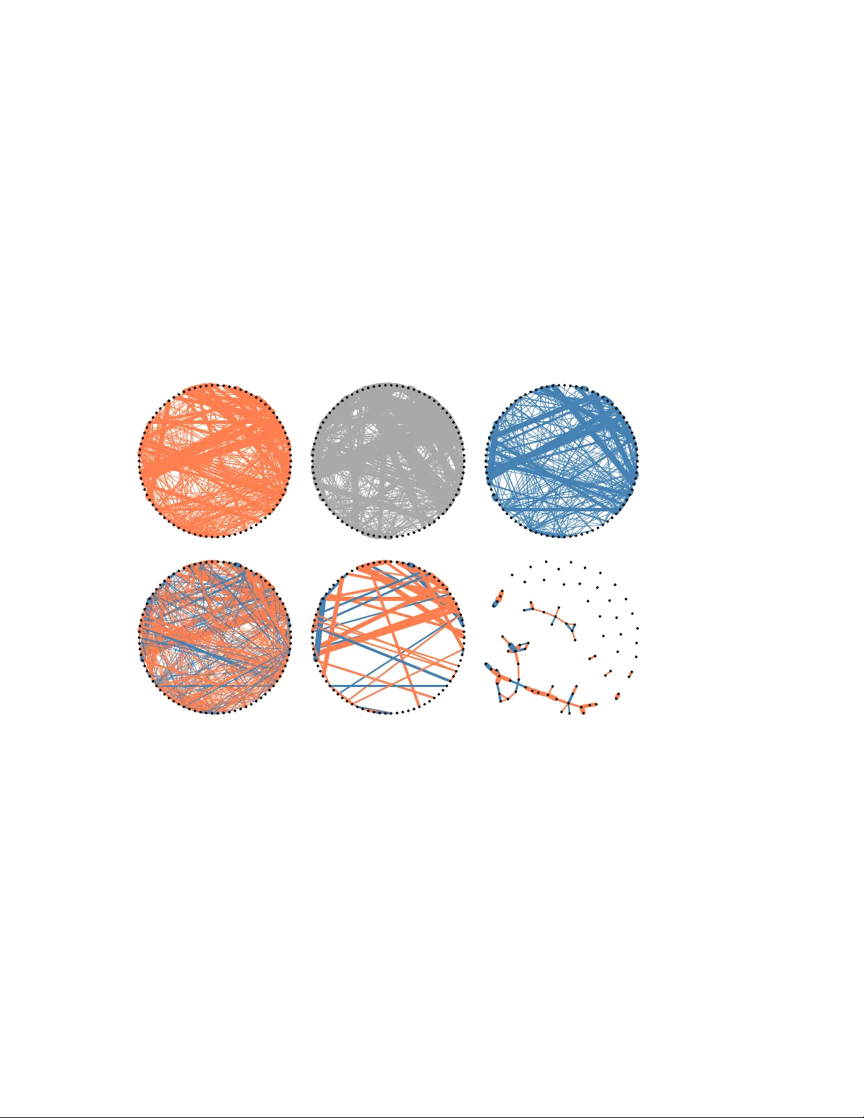
Journal of Machine Learning Research 21 (2020) 1-52 Submitted 10/15; Revised 8/19; Published 3/20 T argeted F used Ridge Estimation of In v erse Co v ariance Matrices from Multiple High-Dimensional Data Classes Anders Ellern Bilgrau F anders.ellern.bilgrau@gmail.com Dep artment of Mathematic al Scienc es, A alb or g University 9220 A alb or g Ø, Denmark & Dep artment of Haematolo gy, A alb or g University Hospital 9000 A alb or g, Denmark Carel F.W. P eeters F cf.peeters@amsterdamumc.nl Dep artment of Epidemiolo gy & Biostatistics, A mster dam University me dic al c enters, lo c ation VUmc Postbus 7057, 1007 MB Amster dam, The Netherlands P oul Sv an te Eriksen sv ante@ma th.aa u.dk Dep artment of Mathematic al Scienc es, A alb or g University 9220 A alb or g Ø, Denmark Martin Bøgsted m boegsted@dcm.aa u.dk Dep artment of Haematolo gy, A alb or g University Hospital 9000 A alb or g, Denmark & Dep artment of Clinic al Me dicine, A alb or g University 9000 A alb or g, Denmark W essel N. v an Wieringen w.v anwieringen@amsterdamumc.nl Dep artment of Epidemiolo gy & Biostatistics, A mster dam University me dic al c enters, lo c ation VUmc Postbus 7057, 1007 MB Amster dam, The Netherlands & Dep artment of Mathematics, VU University Amster dam 1081 HV Amster dam, The Netherlands Editor: F rancis Bac h Abstract W e consider the problem of join tly estimating m ultiple inv erse cov ariance matrices from high-dimensional data consisting of distinct classes. An ` 2 -p enalized maximum lik eliho o d approac h is emplo yed. The suggested approach is ﬂexible and generic, incorp orating sev eral other ` 2 -p enalized estimators as sp ecial cases. In addition, the approach allows sp eciﬁca- tion of target matrices through which prior kno wledge ma y b e incorp orated and whic h can stabilize the estimation procedure in high-dimensional settings. The result is a targeted F . Shared ﬁrst authorship. c  2020 Anders E. Bilgrau, Carel F.W. Peeters, Poul Sv ante Eriksen, Martin Bøgsted, and W essel N. v an Wieringen. License: CC-BY 4.0, see https://creativecommons.org/licenses/by/4.0/ . Attribution requiremen ts are provided at http://jmlr.org/papers/v21/15- 509.html . Bilgrau & Peeters et al. fused ridge estimator that is of use when the precision matrices of the constituent classes are b elieved to chieﬂy share the same structure while p oten tially diﬀering in a num b er of lo cations of interest. It has many applications in (m ulti)factorial study designs. W e fo- cus on the graphical interpretation of precision matrices with the prop osed estimator then serving as a basis for integrativ e or meta-analytic Gaussian graphical mo deling. Situa- tions are considered in which the classes are deﬁned b y data sets and subtypes of diseases. The p erformance of the prop osed estimator in the graphical mo deling setting is assessed through extensive simulation exp eriments. Its practical usabilit y is illustrated by the dif- feren tial net work modeling of 12 large-scale gene expression data sets of diﬀuse large B-cell lymphoma subtypes. The estimator and its related procedures are incorp orated into the R -pac k age rags2ridges . Keyw ords: diﬀeren tial netw ork estimation, Gaussian graphical mo deling, generalized fused ridge, high-dimensional data, ` 2 -p enalized maxim um lik eliho o d, structural meta- analysis 1. In tro duction High-dimensional data are ubiquitous in mo dern statistics. Consequently , the fundamen- tal problem of estimating the cov ariance matrix or its in verse (the precision matrix) has receiv ed renewed atten tion. Supp ose w e hav e n i.i.d. observ ations of a p -dimensional v ari- ate distributed as N p ( µ , Σ ). The Gaussian log-likelihoo d parameterized in terms of the precision matrix Ω = Σ − 1 is then giv en by: L ( Ω ; S ) ∝ ln | Ω | − tr( SΩ ) , (1) where S is the sample co v ariance matrix. When n > p the maximum of (1) is attained at the maximum lik eliho o d estimate (MLE) ˆ Ω ML = S − 1 . How ev er, in the high-dimensional case, i.e., when p > n , the sample cov ariance matrix S is singular and its inv erse ceases to exist. F urthermore, when p ≈ n , the sample cov ariance matrix may b e ill-conditioned and the inv ersion b ecomes numerically unstable. Hence, these situations necessitate usage of regularization techniques. Here, w e study the sim ultaneous estimation of n umerous precision matrices when mul- tiple classes of high-dimensional data are present. Supp ose y ig is a realization of a p - dimensional Gaussian random vector for i = 1 , . . . , n g indep enden t observ ations nested within g = 1 , . . . , G classes, each with class-dependent co v ariance Σ g , i.e., y ig ∼ N p ( µ g , Σ g ) for eac h designated class g . Hence, for each class a data set consisting of the n g × p matrix Y g = [ y 1 g , . . . , y n g g ] > is observ ed. Without loss of generality µ g = 0 can b e assumed as eac h data set Y g can b e centered around its column means. The class-speciﬁc sample co v ariance matrix is given by S g = 1 n g n g X i =1 y ig y > ig = 1 n g Y > g Y g , whic h constitutes the well-kno wn MLE of Σ g as discussed ab ov e. The closely related p o ole d sample cov ariance matrix S • = 1 n • G X g =1 n g X i =1 y ig y > ig = 1 n • G X g =1 n g S g , (2) 2 T argeted Fused Ridge Precision Estima tion where n • = P G g =1 n g , is an oft-used estimate of the common co v ariance matrix across classes. In the high-dimensional setting, in which p > n • (implying p > n g ), the S g and S • are singular and their inv erses do not exist. Our primary interest th us lies in estimating the precision matrices Ω 1 = Σ − 1 1 , . . . , Ω G = Σ − 1 G , as well as their commonalities and diﬀerences, when p > n • . W e will dev elop a general ` 2 -p enalized ML framework to this end whic h we designate tar gete d fuse d ridge estimation . The estimation of multiple precision matrices from high-dimensional data classes is of in terest in many applications. The ﬁeld of oncogenomics, for example, often deals with high-dimensional data from high-throughput exp eriments. Class membership may ha v e diﬀeren t connotations in such settings. It may refer to certain sub-classes within a single data set such as cancer subtypes (cancer is a very heterogeneous disease, even when presen t in a single organ). It ma y also designate diﬀeren t data sets or studies. Likewise, the class indicator may also refer to a conjunction of b oth subclass and study mem b ership to form a t wo-w a y design of factors of interest (e.g., breast cancer subtypes present in a batch of study-sp eciﬁc data sets), as is often the case in oncogenomics. Our approach is th us motiv ated b y the meta-analytic setting, where w e aim for an integrativ e analysis in terms of sim ultaneously considering multiple data (sub-)classes, data sets, or b oth. Its desire is to b orro w statistical p ow er across classes b y eﬀectively increasing the sample size in order to improv e sensitivity and sp eciﬁcit y of discov eries. 1.1 Related Literature There hav e b een man y prop osals for estimating a single precision matrix in high-dimensional data settings. A p opular approach is to amend (1) with an ` 1 -p enalt y (Y uan and Lin, 2007; Banerjee et al., 2008; F riedman et al., 2008; Y uan, 2008). The solution to this p enalized problem is generally referred to as the gr aphic al lasso and it is p opular as it p erforms automatic mo del selection, i.e., the resulting estimate is sparse. It is heavily used in Gaus- sian graphical mo deling (GGM) as the supp ort of a Gaussian precision matrix represents a Mark ov random ﬁeld (Lauritzen, 1996). The ` 1 -approac h has b een extended to deal with more than a single sample-group. Ha et al. (2015) employ ed a tw o-class approach that ﬁrst extracts a global precision matrix b y the graphical lasso after which precision regressions are emplo yed to ﬁnd lo cal diﬀer- ences. Zhao et al. (2014) also regard the t wo-class setting but, in contrast to many other approac hes, fo cus on direct estimation of the diﬀerence betw een tw o precision matrices. Man y w orks also mov e b eyond the tw o-class setting. Guo et al. (2011) hav e prop osed a parametrization of class-sp eciﬁc precision matrices that expresses the individual elements as a pro duct of shared and class-sp eciﬁc factors. They include ` 1 -p enalties on b oth the shared and class-sp eciﬁc factors in order to jointly estimate the sparse precision matrices (represen ting graphical mo dels). The p enalty on the shared factors promotes a shared sparsit y structure while the p enalt y on the class-sp eciﬁc factors promotes class-sp eciﬁc de- viations from the shared sparsity structure. Danaher et al. (2014) ha ve generalized these eﬀorts by prop osing the joint gr aphic al lasso which allo ws for v arious p enalty structures. They study tw o particular choices: the gr oup gr aphic al lasso that encourages a shared spar- sit y structure across the class-sp eciﬁc precision matrices, and the fuse d gr aphic al lasso that promotes a shared sparsity structure as well as shared precision elemen t-v alues. 3 Bilgrau & Peeters et al. The metho ds that mo v e b eyond the t wo-class setting ha v e in common that they (implic- itly) assume the same degree of similarit y b etw een all p ossible pairs of precision matrices. Tw o recen t works pro vide an imp ortant generalization by allo wing for v arying degrees of similarit y: Peterson et al. (2015) and Saegusa and Sho jaie (2016). These w orks p ermit, resp ectiv ely from a Bay esian and frequentist p ersp ectiv e, for the pair-sp eciﬁc similarities to b e estimated from the data. Our motiv ation is related to these w orks (see Section 1.2). A hypothesis testing literature on multiple high-dimensional precision matrices has de- v elop ed concurrently with the estimation literature. Generally , the testing approaches are supp orted by p enalized estimation. As in estimation, the approac hes can b e demarcated b y either a global or a lo cal thrust (Cai, 2017). The former fo cuses on testing the o verall diﬀerence b et ween tw o precision matrices. The latter focuses on the simultaneous testing of the non-redundant individual entries of the diﬀerence matrix b etw een tw o precision ma- trices. St¨ adler and Mukherjee (2017) provide a tw o-sample global testing approach under a sparsit y assumption. Xia et al. (2015) provide b oth a global test as well as lo cal testing through a (sparse) regression approac h. See Cai (2017) for a review of recen t w ork in testing for high-dimensional co v ariance and precision structures. 1.2 Motiv ation of Approach T esting of high-dimensional precision matrices is generally only p ow erful when the alterna- tiv e is sparse. How ev er, sparsit y need not necessarily b e a tenable assumption. Moreo v er, the testing approaches are conﬁned to tw o-class settings. Hence, we fo cus on estimation. Our goal is to pro vide a multiple class join t-estimation metho d that do es not dep end on a sparsit y assumption and that allo ws for the ﬂexible incorp oration of prior information. W e motiv ate our approac h b elo w. While simultaneous estimation and mo del selection can b e deemed elegant, automatic sparsit y is not alw ays an asset. It may b e that one is in trinsically interested in more accurate represen tations of class-sp eciﬁc precision matrices in the high-dimensional situa- tion. By ‘intrinsically’ we mean a represen tation that do es not assume a (sp eciﬁc) sparsit y pattern or structure. Suc h representations are useful in enabling in the high-dimensional setting (standard) statistical applications directly dep endent on the precision matrix, suc h as cov ariance-regularized regression (Witten and Tibshirani, 2009) or discriminant analysis (Price et al., 2015). One is then not after sparse representations, but rather (relatively) lo w-v ariance representations of the precision(s) in high-dimension. It is then natural to prefer usage of a regularization metho d that shrinks the estimated elements of the precision matrices prop ortionally . In addition, when indeed considering netw ork representations of data (suc h that some lev el of sparsit y is ultimately desired), one need not necessarily prefer the encouragement of sparsity through an ` 1 -approac h. It is well-kno wn that ` 1 -based supp ort recov ery and estimation is consisten t only under the assumption that the true (diﬀerential) graphical mo del is (very) sparse. The ` 1 -p enalt y is unable to retriev e the sparsity pattern when the num ber of truly non-n ull elements exceeds the av ailable sample size (v an Wieringen and Peeters, 2016). This can b e termed undesirable as there is accum ulating evidence that many net w orks traditionally represented b y graphical mo dels, suc h as bio chemical path wa ys gov erning disease aetiology and progression, are dense (Boyle et al., 2017). In 4 T argeted Fused Ridge Precision Estima tion suc h a situation one may wish to couple a non-sparsity-inducing p enalt y with a p ost-ho c selection step allo wing for probabilistic control ov er element selection (v an Wieringen and P eeters, 2016). W e therefore consider ` 2 or ridge-type penalization. The ` 2 -approac h we consider will b e tar gete d in the sense that it allo ws for the sp eciﬁ- cation of (p ossibly class-sp e ciﬁc) target matrices that ma y enco de prior information. The motiv ation for including targets in general is that well-informed choices of the target can greatly improv e the estimation in terms of loss/risk (Section 5). In addition, our framework also allows for v arying degrees of similarity b etw een (all p ossible) pairs of class-sp eciﬁc pre- cision matrices through the incorp oration of a p enalty matrix (Section 2). The diagonal elemen ts of this matrix determine the rates of shrink age of the class-sp eciﬁc precision ma- trices tow ards their corresp onding targets while the oﬀ-diagonal entries determine the rates of pair-sp eciﬁc fusion. The prop osed framew ork is th us ﬂexible in the sense that it allows for the incorp oration of prior information along tw o roads as well as their interpla y: (i) via the target matrices, and (ii) via the p enalty matrix. A t one end of the sp ectrum we can include weak prior information through uninformativ e shared target matrices while letting the similarities b etw een all pairs of precision matrices b e subsequently determined b y the data (analogously to P eterson et al., 2015; Saegusa and Sho jaie, 2016). At the other end w e can include strong prior knowledge through informative class-sp eciﬁc target matrices while imp osing restrictions on class-sp eciﬁc similarities b y imp osing (exclusion) constrain ts on the penalty matrix. 1.3 Overview Section 2 presen ts the tar gete d fuse d ridge estimation framework. The prop osed fused ` 2 -p enalt y allows for the sim ultaneous estimation of multiple precision matrices from high- dimensional data classes that chieﬂy share the same structure but that may diﬀerentiate in lo cations of interest. The usage of the mentioned target and p enalty matrices makes the framew ork ﬂexible and general. It contains the recent w ork of Price et al. (2015) and v an Wieringen and P eeters (2016) as special cases. It ma y also be view ed as an ` 2 -generalization of the work of Danaher et al. (2014). Moreov er, the framew ork can b e view ed as bridging the work of Danaher et al. (2014) and Saegusa and Sho jaie (2016), by allowing v arying degrees of class-sp eciﬁc similarities, ranging from completely ﬁxed for all possible pairs to completely data-determined for all p ossible pairs. In the same v ein, it may b e viewed as a computationally feasible alte rnativ e to the work of P eterson et al. (2015), as it allo ws for the incorp oration of prior information without having to formally sp ecify prior distributions. As such it ev ades the computational burden of a full Bay es approach. The metho d is con tingent up on the selection of penalty v alues and target matrices, topics that are treated in Section 3. This section shows how—through the penalty v alues and target matrices—v arying levels of sp eciﬁcity ma y b e incorp orated. Section 4 then fo cuses on the graphical interpretation of precision matrices. It shows how the fused ridge precision estimates may b e coupled with p ost-ho c supp ort determination in order to arrive at m ultiple graphical mo dels. W e will refer to this coupling as the fuse d gr aphic al ridge . This then serv es as a basis for in tegrative or meta-analytic net w ork mo deling. Section 5 then assesses the p erformance of the proposed estimator through extensiv e simulation exp erimen ts. These simulations sho w that the inclusion of target matrices can impro v e 5 Bilgrau & Peeters et al. estimation eﬃciency . Section 6 illustrates the techniques by applying it in a large scale in tegrative study of gene expression data of diﬀuse large B-cell lymphoma. The focus is then on ﬁnding common motifs and motif diﬀerences in netw ork representations of (deregulated) molecular path wa ys. The analysis sho ws the added v alue of the targeted fusion approach to integration by juxtaposing it with a nonintegrativ e approach. Moreov er, it shows ho w pilot data and database information can b e com bined to provide eﬀective target matrices. Section 7 concludes with a discussion. 1.4 Notation Some additional notation m ust b e in tro duced. Throughout the text and supplementary material, we use the follo wing notation for certain matrix prop erties and sets: W e use A  0 and B  0 to denote symmetric p ositive deﬁnite and p ositive semi-deﬁnite matrices A and B , resp ectively . By R , R + , and R ++ w e denote the real num b ers, the non-negative real num b ers, and the strictly p ositiv e real n umbers, resp ectively . In notational analogue, S p , S p + , and S p ++ are used to denote the space of p × p real symmetric matrices, the real symmetric p ositive semi-deﬁnite matrices, and real symmetric p ositive deﬁnite matrices, resp ectiv ely . That is, e.g., S p ++ = { X ∈ R p × p : X = X > ∧ X  0 } . Negativ e subscripts similarly denote negativ e reals and negative deﬁniteness. By A ≥ B and similar w e denote element-wise relations, i.e., ( A ) j q ≥ ( B ) j q for all ( j, q ). Matrix subscripts will usually denote class membership, e.g., A g denotes (the realization of ) matrix A in class g . F or notational brevity we will often use the shorthand { A g } to denote the set { A g } G g =1 . The following notation is used throughout for op erations: W e write diag( A ) for the column vector comp osed of the diagonal of A and v ec( A ) for the v ectorization op erator whic h stacks the columns of A on top of each other. Moreov er, ◦ will denote the Hadamard pro duct while ⊗ refers to the Kroneck er pro duct. W e will also rep eatedly mak e use of several special matrices and functions. W e let I p denote the ( p × p )-dimensional identit y matrix. Similarly , J p will denote the ( p × p )- dimensional all-ones matrix. In addition, 0 will denote the null-matrix, the dimensions of whic h should b e clear from the context. Lastly , k · k 2 F and 1 [ · ] will stand for the squared F rob enius norm and the indicator function, resp ectively . 2. T argeted F used Ridge Estimation In this section we ﬁrst give a general formulation of the targeted fused ridge estimation problem (Section 2.1). Next, the maximizing class-speciﬁc argument is explored as w ell as its prop erties (Section 2.2). Last, an algorithm is presented with whic h the general, m ultiple-class solution can b e obtained (Section 2.3). 2.1 A General Penalized Log-Likelihoo d Problem Supp ose G classes of ( n g × p )-dimensional data exist and that the samples within e ac h class are i.i.d. normally distributed. The log-likelihoo d for the data takes the follo wing form under the additional assumption that all n • observ ations are indep endent: L ( { Ω g } ; { S g } ) ∝ X g n g  ln | Ω g | − tr( S g Ω g )  . (3) 6 T argeted Fused Ridge Precision Estima tion W e desire to obtain estimates { ˆ Ω g } ∈ S p ++ of the precision matrices for eac h class. Though not a requiremen t, we primarily consider situations in whic h p > n g for all g , necessitating the need for regularization. T o this end, amend (3) with the fuse d ridge p enalty given b y f FR ( { Ω g } ; { λ g 1 g 2 } , { T g } ) = X g λ g g 2   Ω g − T g   2 F + X g 1 ,g 2 λ g 1 g 2 4   ( Ω g 1 − T g 1 ) − ( Ω g 2 − T g 2 )   2 F , (4) where the T g ∈ S p + indicate kno wn class-sp eciﬁc tar get matric es (see also Section 3.3), the λ g g ∈ R ++ denote class-sp eciﬁc ridge p enalty p ar ameters , and the λ g 1 g 2 ∈ R + are pair-sp eciﬁc fusion p enalty p ar ameters sub ject to the requirement that λ g 1 g 2 = λ g 2 g 1 . All p enalties can then b e conv enien tly summarized into a non-negative symmetric matrix Λ = [ λ g 1 g 2 ] whic h we call the p enalty matrix . The diagonal of Λ corresp onds to the class- sp eciﬁc ridge p enalties whereas oﬀ-diagonal entries are the pair-sp eciﬁc fusion penalties. The rationale and use of the p enalt y matrix is motiv ated further in Section 3.1. Com bining (3) and (4) yields a general targeted fused ridge estimation problem: arg max { Ω g }∈S p ++ ( L ( { Ω g } ; { S g } ) − X g λ g g 2   Ω g − T g   2 F − X g 1 ,g 2 λ g 1 g 2 4   ( Ω g 1 − T g 1 ) − ( Ω g 2 − T g 2 )   2 F ) . (5) The problem of (5) is strictly concav e. F urthermore, it is worth noting that non-zero fusion p enalties, λ g 1 g 2 > 0 for all g 1 6 = g 2 , alone will not guaran tee uniqueness when p > n • : In high dimensions, all ridge p enalties λ g g should b e strictly p ositive to ensure iden tiﬁability . These and other prop erties of the estimation problem are review ed in Section 2.2. The problem stated in (5) is v ery general. W e shall sometimes consider a single common ridge p enalty λ g g = λ for all g , as well as a common fusion penalty λ g 1 g 2 = λ f for all class pairs g 1 6 = g 2 (cf., ho wev er, Section 3.1) such that Λ = λ I G + λ f ( J G − I G ). This simpliﬁcation leads to the ﬁrst sp ecial case: arg max { Ω g }∈S p ++ ( L ( { Ω g } ; { S g } ) − λ 2 X g   Ω g − T g   2 F − λ f 4 X g 1 ,g 2   ( Ω g 1 − T g 1 ) − ( Ω g 2 − T g 2 )   2 F ) . Here and analogous to (5), λ controls the rate of shrink age of each precision Ω g to wards the corresp onding target T g (v an Wieringen and P eeters, 2016), while λ f determines the retainmen t of entry-wise similarities b etw een ( Ω g 1 − T g 1 ) and ( Ω g 2 − T g 2 ) for all class pairs g 1 6 = g 2 . When T g = T for all g , the problem further simpliﬁes to arg max { Ω g }∈S p ++ ( L ( { Ω g } ; { S g } ) − λ 2 X g   Ω g − T   2 F − λ f 4 X g 1 ,g 2   Ω g 1 − Ω g 2   2 F ) , (6) where the targets are seen to disappear from the fusion term. Lastly , when T = 0 the problem (6) reduces to its simplest form recen tly considered by Price et al. (2015). App endix A studies, in order to supp ort an intuitiv e feel for the fused ridge estimation problem, its geometric interpretation in this latter con text. 7 Bilgrau & Peeters et al. 2.2 Estimator and Prop erties There is no explicit solution to (5) except for certain sp ecial cases and thus an iterative optimization pro cedure is needed for its general solution. As describ ed in Section 2.3, w e employ a coordinate ascent pro cedure which relies on the conca vit y of the p enalized lik eliho o d (see Lemma 10 in App endix B.1) and rep eated use of the following result, whose pro of (as indeed all pro ofs) has b een deferred to App endix B.2: Prop osition 1 L et { T g } ∈ S p + and let Λ ∈ S G b e a ﬁxe d p enalty matrix such that Λ ≥ 0 and diag ( Λ ) > 0 . F urthermor e, assume that Ω g is p ositive deﬁnite and ﬁxe d for al l g 6 = g 0 . The maximizing ar gument for class g 0 of the optimization pr oblem (5) is then given by ˆ Ω g 0  Λ , { Ω g } g 6 = g 0  = (  ¯ λ g 0 I p + 1 4  ¯ S g 0 − ¯ λ g 0 ¯ T g 0  2  1 / 2 + 1 2  ¯ S g 0 − ¯ λ g 0 ¯ T g 0  ) − 1 , (7) wher e ¯ S g 0 = S g 0 − X g 6 = g 0 λ g g 0 n g 0 ( Ω g − T g ) , ¯ T g 0 = T g 0 , and ¯ λ g 0 = λ g 0 • n g 0 , (8) with λ g 0 • = P g λ g g 0 denoting the sum of the g 0 th c olumn (or r ow) of Λ . Remark 2 Deﬁning ¯ T g 0 = T g 0 in Pr op osition 1 may b e de eme d r e dundant. However, it al lows us to state e quivalent alternatives to (8) without c onfusing notation. Se e Se ction 2.3 as wel l as App endix B.2 and Se ction 1 of the Supplementary Material. Remark 3 The tar get matric es fr om Pr op osition 1 may b e chosen nonne gative deﬁnite. However, cho osing n.d. tar gets may le ad to il l-c onditione d estimates in the limit. F r om a shrinkage p ersp e ctive we thus pr efer to cho ose { T g } ∈ S p ++ . Se e Se ction 3.3. Prop osition 1 pro vides a function for up dating the estimate of the g 0 th class while ﬁx- ing the remaining parameters. As a sp ecial case, consider the following. If all oﬀ-diagonal elemen ts of Λ are zero no ‘class fusion’ of the estimates takes place and the maximiza- tion problem decouples into G individual, disjoint ridge estimations: See Corollary 11 in App endix B.2. The next result summarizes some prop erties of (7): Prop osition 4 Consider the estimator of Pr op osition 1 and its ac c omp anying assumptions. L et ˆ Ω g ≡ ˆ Ω g  Λ , { Ω g 0 } g 0 6 = g  b e the pr e cision matrix estimate of the g th class. F or this estimator, the fol lowing pr op erties hold: i. ˆ Ω g  0 for al l λ g g ∈ R ++ ; ii. lim λ gg → 0 + ˆ Ω g = S − 1 g if P g 0 6 = g λ g g 0 = 0 and p ≤ n g ; iii. lim λ gg →∞ − ˆ Ω g = T g if λ g g 0 < ∞ for al l g 0 6 = g ; iv. lim λ g 1 g 2 →∞ − ( ˆ Ω g 1 − T g 1 ) = lim λ g 1 g 2 →∞ − ( ˆ Ω g 2 − T g 2 ) if λ g 0 1 g 0 2 < ∞ for al l { g 0 1 , g 0 2 } 6 = { g 1 , g 2 } . 8 T argeted Fused Ridge Precision Estima tion The ﬁrst item of Prop osition 4 implies that strictly positive λ g g are suﬃcien t to guaran tee p ositiv e deﬁnite estimates from the ridge estimator. The second item implies that if ‘class fusion’ is absent, then one obtains the standard MLE S − 1 g as the right-hand limit for group g , whose existence is only guaran teed when p ≤ n g . The third item sho ws that the fused ridge precision estimator for class g is shrunken exactly to its target matrix when the ridge p enalt y tends to inﬁnity while the fusion p enalties do not. The last item shows that the precision estimators of any tw o classes tend to a common estimate when the fusion p enalty b et ween them tends to inﬁnity while all remaining penalty parameters remain ﬁnite. The attractiveness of the general estimator hinges up on the eﬃciency by whic h it can b e obtained. W e state a result useful in this respec t before turning to our computational approac h in Section 2.3: Prop osition 5 L et ˆ Ω g ≡ ˆ Ω g  Λ , { Ω g 0 } g 0 6 = g  b e the pr e cision matrix estimate (7) for the g th class and deﬁne [ ˆ Ω g ] − 1 ≡ ˆ Σ g . The estimate ˆ Ω g c an then b e obtaine d without inversion thr ough: ˆ Ω g = 1 ¯ λ g h ˆ Σ g − ( ¯ S g − ¯ λ g ¯ T g ) i = 1 ¯ λ g (  ¯ λ g I p + 1 4  ¯ S g − ¯ λ g ¯ T g 0  2  1 / 2 − 1 2  ¯ S g − ¯ λ g ¯ T g  ) . Remark 6 Note that Pr op osition 5 implies that our fr amework also imme diately pr ovides for r e gularize d class-sp e ciﬁc estimates of c ovarianc e matric es as ˆ Σ g = ¯ λ g ˆ Ω g + ( ¯ S g − ¯ λ g ¯ T g ) . Its pr op erties ar e analo gous to those state d in Pr op osition 4. 2.3 Algorithm Equation (7) allows for up dating the precision estimate ˆ Ω g of class g b y plugging in the remaining ˆ Ω 0 g , g 0 6 = g , and assuming them ﬁxed. Hence, from initial estimates, all preci- sion estimates may b e iterativ ely up dated un til some conv ergence criterion is reached. W e prop ose a blo c k coordinate ascen t pro cedure to solv e (5) b y rep eated use of the results in Prop osition 1. This pro cedure is outlined in Algorithm 1. By the strict concavit y of the problem in (5), the pro cedure guarantees that, con tingen t up on conv ergence, the unique maximizer is attained when considering all ˆ Ω g join tly . Moreov er, we can state the following result: Prop osition 7 The gr adient asc ent pr o c e dur e given in Algorithm 1 wil l always stay within the r e alm of p ositive deﬁnite matric es S p ++ . The pro cedure is implemen ted in the rags2ridges pac k age within the R statistical language ( R Core T eam, 2012). This implementation fo cuses on stability and eﬃciency . With regard to the former: Equiv alen t (in terms of the obtained estimator) alternatives to (8) can b e deriv ed that are numerically more stable for extreme v alues of Λ . The most apparen t suc h alternative is: ¯ S g 0 = S g 0 , ¯ T g 0 = T g 0 + X g 6 = g 0 λ g g 0 λ g 0 • ( Ω g − T g ) , and ¯ λ g 0 = λ g 0 • n g 0 . (9) It ‘up dates’ the target ¯ T g instead of the sample cov ariance ¯ S g and has the intuitiv e in- terpretation that the target matrix for a giv en class in the fused case is a combination 9 Bilgrau & Peeters et al. of the actual class target matrix and the ‘target corrected’ estimates of remaining classes. The implemen tation makes use of this alternative where appropriate. See Section 1 of the Supplemen tary Material for details on alternative up dating schemes. Algorithm 1 Pseudo co de for the fused ridge blo c k co ordinate ascent pro cedure. 1: Input: 2: Suﬃcient data: ( S 1 , n 1 ) , . . . , ( S G , n G ) 3: Penalty matrix: Λ 4: Conver genc e criterion: ε > 0 5: Output: 6: Estimates: ˆ Ω 1 , . . . , ˆ Ω G 7: pro cedure ridgeP.fused ( S 1 , . . . , S G , n 1 , . . . , n G , Λ , ε ) 8: Initialize : ˆ Ω (0) g for all g . 9: for c = 1 , 2 , 3 , . . . do 10: for g = 1 , 2 , . . . , G do 11: Up date ˆ Ω ( c ) g := ˆ Ω g  Λ , ˆ Ω ( c ) 1 , . . . , ˆ Ω ( c ) g − 1 , ˆ Ω ( c − 1) g +1 , . . . , ˆ Ω ( c − 1) G  b y (7). 12: end for 13: if max g n k ˆ Ω ( c ) g − ˆ Ω ( c − 1) g k 2 F k ˆ Ω ( c ) g k 2 F o < ε then 14: return  ˆ Ω ( c ) 1 , . . . , ˆ Ω ( c ) G  15: end if 16: end for 17: end pro cedure The w orst-case asymptotic time complexity of the pro cedure is O ( p 3 ) due to the necessity of the matrix square root. Eﬃciency is then secured through v arious roads. First, in certain sp ecial cases closed-form solutions to (5) exist. When appropriate, these explicit solutions are used. Moreo ver, these solutions ma y pro vide warm-starts for the general problem. See Section 2 of the Supplemen tary Material for details on estimation in these sp ecial cases. Sec- ond, the result from Prop osition 5 is used, meaning that the relatively exp ensive op eration of matrix inv ersion is a voided. Third, additional computational sp eed was achiev ed by imple- men ting core op erations in C++ via the R -pack ages Rcpp and RcppArmadillo (Sanderson, 2010; Eddelbuettel and F ran¸ cois, 2011; F ran¸ cois et al., 2012; Eddelbuettel, 2013). These eﬀorts make analyzes with large p feasible. Throughout, we will initialize the algorithm with ˆ Ω (0) g = p/ tr( S • ) · I p for all g . 3. P enalt y and T arget Selection In this section w e discuss selection of the penalty parameters and the target matrices. First, w e discuss, b y w ay of examples, ho w the penalty matrix connects to a p enalty-graph and ho w its structure ma y encode prior information in the analysis of v arious study-designs (Section 3.1). Next, we present sev eral computational approac hes to select optimal v alues for the parameters in the (p ossibly structured) p enalt y matrix (Section 3.2). Last, w e giv e sev eral considerations in choosing target matrices (Section 3.3). 10 T argeted Fused Ridge Precision Estima tion 3.1 The Penalt y Graph and Analysis of F actorial Designs Equalit y of all class-sp eciﬁc ridge p enalties λ g g is deemed restrictive, as is equalit y of all pair-sp eciﬁc fusion p enalties λ g 1 g 2 . In many settings, suc h as the analysis of factorial designs, ﬁner control ov er the individual v alues of λ g g and λ g 1 g 2 b eﬁts the analysis. This will b e motiv ated by sev eral examples of increasing complexity . In order to do so, some additional notation is dev elop ed: The p enalties of Λ can b e summarized b y a no de- and edge-weigh ted graph P = ( W, H ) where the vertex set W corresp onds to the p ossible classes and the edge set H corresp onds to the similarities to b e retained. The weigh t of no de g ∈ W is given by λ g g and the w eight of edge ( g 1 , g 2 ) ∈ H is then giv en b y λ g 1 g 2 . W e refer to P as the p enalty gr aph asso ciated with the p enalty matrix Λ . The p enalty graph P is simple and undirected as the penalty matrix is symmetric. In the examples b elo w w e generally assume p > n • . Example 1 Consider G = 2 classes or subtyp es ( ST ) of diﬀuse lar ge B-c el l lymphoma (DLBCL) p atients with tumors r esembling either so-c al le d activate d B-c el ls ( ABC ) or ger- minal c entr e B-c el ls ( GCB ). Patients with the latter subtyp e have sup erior over al l survival (A lizadeh et al., 2000). As the GCB phenotyp e is mor e c ommon than ABC , one might imagine a sc enario wher e the two class sample sizes ar e suﬃciently diﬀer ent such that n GCB  n ABC . Numeric pr o c e dur es to obtain a c ommon ridge p enalty (se e, e.g., Se ction 3.2) would then b e dominate d by the smal ler gr oup. Henc e, cho osing non-e qual class ridge p enalties for e ach gr oup wil l al low for a b etter analysis. In such a c ase, the fol lowing p enalty gr aph and matrix would b e suitable: P = λ 11 ABC λ 22 GCB λ f Λ =  λ 11 λ f λ f λ 22  . (10) Example 2 Consider data fr om a one-way factorial design wher e the factor is or dinal with classes A , B , and C . F or simplicity, we cho ose the same ridge p enalty λ for e ach class. Say we have prior information that A is closer to B and B is closer to C than A is to C . The fusion p enalty on the p airs c ontaining the interme diate level B might then b e al lowe d to b e str onger. The fol lowing p enalty gr aph and matrix ar e thus sensible: P = λ A λ C λ B λ B λ B λ AC Λ =   λ λ B λ AC λ B λ λ B λ AC λ B λ   . (11) Dep ending on the applic ation, one might even omit the dir e ct shrinkage b etwe en A and C by ﬁxing λ AC = 0 . A similar p enalty scheme might also b e r elevant if one class of the factor is an unknown mix of the r emaining classes and one wishes to b orr ow statistic al p ower fr om such a class. Example 3 In two-way or n -way factorial designs one might wish to r etain similarities in the ‘dir e ction ’ of e ach factor along with a factor-sp e ciﬁc p enalty. Consider, say, 3 onc o ge- nomic data sets ( DS 1 , DS 2 , DS 3 ) r e gar ding ABC and GCB DLBCL c anc er p atients. This 11 Bilgrau & Peeters et al. yields a total of G = 6 classes of data. One choic e of p enalization of this 2 by 3 design is r epr esente d by the p enalty gr aph and matrix b elow: P = λ λ λ λ λ λ λ DS λ DS λ DS λ DS λ ST λ ST λ ST λ DS λ DS DS 1 DS 2 DS 3 GCB ABC Λ =         λ λ DS λ DS λ ST 0 0 λ DS λ λ DS 0 λ ST 0 λ DS λ DS λ 0 0 λ ST λ ST 0 0 λ λ DS λ DS 0 λ ST 0 λ DS λ λ DS 0 0 λ ST λ DS λ DS λ         . (12) This example would favor similarities (with the same for c e) only b etwe en p airs sharing a c ommon level in e ach factor. This ﬁner c ontr ol al lows users, or the employe d algorithm, to p enalize diﬀer enc es b etwe en data sets mor e (or less) str ongly than diﬀer enc es b etwe en the ABC and GCB sub-classes. This c orr esp onds to not applying dir e ct shrinkage of inter action eﬀe cts which is of inter est in some situations. While the p enalty graph primarily serves as an in tuitive ov erview, it do es provide some aid in the construction of the p enalty matrix for m ultifactorial designs. F or example, the construction of the penalty matrix (12) in Example 3 corresponds to a Cartesian graph pro duct of t w o complete graphs similar to those given in (10) and (11). W e state that P and Λ should b e chosen carefully in conjunction with the c hoice of target matrices. Ideally , only strictly necessary p enalization parameters (from the p ersp ectiv e of the desired analysis) should b e in tro duced. Eac h additional p enalty introduced will increase the diﬃcult y of ﬁnding the optimal p enalty v alues by increasing the dimension of the searc h-space. 3.2 Selection of Penalt y Parameters As the ` 2 -p enalt y do es not automatically induce sparsity in the estimate, it is natural to seek loss eﬃciency . W e then use cross-v alidation (CV) for p enalt y parameter selection due to its relation to the minimization of the Kullbac k-Leibler divergence and its predictive accuracy stemming from its data-driven nature. W e randomly divide the data of each class in to k = 1 , . . . , K disjoin t subsets of approximately the same size. Previously , we ha ve deﬁned ˆ Ω g ≡ ˆ Ω g  Λ , { Ω g 0 } g 0 6 = g  to b e the precision matrix estimate of the g th class. Let ˆ Ω ¬ k g b e the analogous estimate (with similar notational dep endencies) for class g based on all samples not in k . Also, let S k g denote the sample cov ariance matrix for class g based on the data in subset k and let n k g denote the size of subset k in class g . The K -fold CV score for our fused regularized precision estimate based on the ﬁxed p enalty Λ can then b e given as: K CV ( Λ ) = 1 K G G X g =1 K X k =1 n k g h − ln | ˆ Ω ¬ k g | + tr( ˆ Ω ¬ k g S k g ) i = − 1 K G G X g =1 K X k =1 L k g  ˆ Ω ¬ k g ; S k g  . One would then c ho ose Λ ∗ suc h that Λ ∗ = arg min Λ K CV ( Λ ) , sub ject to: Λ ≥ 0 ∧ diag( Λ ) > 0 . (13) 12 T argeted Fused Ridge Precision Estima tion The least biased predictive accuracy can b e obtained by c ho osing K = n g suc h that n k g = 1. This w ould give the fused version of leav e-one-out CV (LOOCV). Unfortunately , LOOCV is computationally demanding for large p and/or large n g . W e prop ose to select the p enal- ties by the computationally exp ensiv e LOOCV only if adequate computational pow er is a v ailable. In cases where it is not, w e propose tw o alternativ es. Our ﬁrst alternativ e is a sp ecial version of the LOOCV scheme that signiﬁcantly re- duces the computational cost. The sp e cial LOOCV (SLOOCV ) is computed m uch like the LOOCV. How ev er, only the class estimate in the class of the omitted datum is up dated. More sp eciﬁcally , the SLOOCV problem is giv en b y: Λ  = arg min Λ SLOOCV( Λ ) , sub ject to: Λ ≥ 0 ∧ diag ( Λ ) > 0 , (14) with SLOOCV( Λ ) = − 1 n • G X g =1 n g X i =1 L i g  e Ω ¬ i g ; S i g  . The estimate e Ω ¬ i g in (14) is obtained b y up dating only ˆ Ω g using Prop osition 1. F or all other g 0 6 = g , e Ω ¬ i g 0 = ˆ Ω g . The motiv ation for the SLOOCV is that a single observ ation in a given class g do es not exert hea vy direct inﬂuence on the estimates in the other classes. This wa y the num b er of fused ridge estimations for each given Λ and eac h giv en leav e- one-out sample is reduced from n • to G estimations. Our second and fastest alternativ e is an approximation of the fused LOOCV score. This approximation can b e used as an alternativ e to (S)LOOCV when the class sample sizes are relativ ely large (precisely the scenario where LOOCV is unfeasible). See Section 3 of the Supplementary Material for detailed information on this approximation. 3.3 Choice of T arget Matrices The target matrices { T g } can b e used to enco de prior information and their c hoice is highly dep enden t on the application at hand. As they inﬂuence the eﬃcacy as well as the amount of bias of the estimate, it is of some imp ortance to make a well-informed choice. Here, we describ e several options of increasing lev el of informativ eness, sho w casing the ﬂexibilit y of target sp eciﬁcation. The limited fused ridge problem in Price et al. (2015) corresp onds to c ho osing the common target T g = T = 0 . This can b e considered the least informative target p ossible. W e generally argue against the use of the non p ositiv e deﬁnite target T = 0 , as it implies shrinking the class precision matrices tow ards the n ull matrix and th us tow ards inﬁnite v ariance. In some situations one ma y wis h to p enalize the diagonal elements of the precision matrices at a diﬀeren t rate than the oﬀ-diagonal elemen ts. Sp ecifying T g = ( S g ◦ I p ) − 1 w ould be equiv alent to shrinking the precision estimate for class g to w ards a diagonal matrix carrying the inv erse v ariances of S g and, hence, (from the precision-p ersp ectiv e) letting the diagonal elements of S g go unp enalized. Suc h a target can b e scaled to giv e v arying rates of shrink age for the (oﬀ-)diagonal elements. That is, one could sp ecify γ g ( S g ◦ I p ) − 1 with γ g ∈ [0 , ∞ ), although from an empirical p ersp ective it w ould make sense to choose γ g ∈ [0 , 1]. 13 Bilgrau & Peeters et al. In the sp ecial case when T g = T for all g one could c hoose T = γ ( S • ◦ I p ) − 1 . When c ho osing γ g = 0 for all g , the common target T g = T = 0 ensues. In the non-fused setting, the consideration of a scalar target matrix T = α I p for some α ∈ [0 , ∞ ) leads to a computational b eneﬁt stemming from the property of rotation equiv ariance (v an Wieringen and P eeters, 2016): Under suc h targets the ridge estimator only operates on the eigen v alues of the sample co v ariance matrix. This b eneﬁt transfers to the fused setting for the estimator describ ed in Prop osition 1. T o see this let V g D ( ¯ S g ) V T g b e the sp ectral decomp osition of ¯ S g with D ( ¯ S g ) denoting a diagonal matrix with the eigen v alues of ¯ S g on the diagonal and where V g denotes the matrix that con tains the corresp onding eigen vectors as columns. Naturally , the orthogonalit y of V g implies V g V T g = V T g V g = I p . Now, note that, if T g = α g I p , we can write ˆ Ω g  Λ , { Ω g 0 } g 0 6 = g  as: V g (  ¯ λ g I p + 1 4  D ( ¯ S g ) − ¯ λ g α g I p  2  1 / 2 + 1 2  D ( ¯ S g ) − ¯ λ g α g I p  ) − 1 V T g . Letting d ( · ) j j denote the j th eigenv alue of the matrix terms in brac kets we th us hav e that: d h ˆ Ω g  Λ , { Ω g 0 } g 0 6 = g  i j j = ( r ¯ λ g + 1 4  d ( ¯ S g ) j j − ¯ λ g α g  2 + 1 2  d ( ¯ S g ) j j − ¯ λ g α g  ) − 1 . Prop osition 4. iii then implies that if λ g g 0 < ∞ for all g 0 6 = g , d h ˆ Ω g  Λ , { Ω g 0 } g 0 6 = g  i j j → α g as λ g g → ∞ − , for all j . Hence, using scalar target matrices implies shrinking the eigen v alues of the class-speciﬁc estimated precision matrix to the cen tral v alue α g . One may consider T g = α g I p with α g ∈ [0 , ∞ ) for eac h g . The rotation equiv ariance prop ert y dictates that it is sensible to c ho ose α g based on empirical information regarding the eigenv alues of S g . One such c hoice could b e the av erage of the recipro cals of the non-zero eigenv alues of S g . A straigh tforward alternative would b e to c ho ose α g = [tr( S g ) /p ] − 1 . In the sp e cial case of (6) where all α g = α the analogous c hoice would b e α = [tr( S • ) /p ] − 1 . The limited fused ridge problem in Price et al. (2015) corresp onds to choosing α g = 0 for all g , suc h that (again) a common target T g = T = 0 is employ ed. More informative targets would mov e b eyond diagonal targets such as the scalar ma- trix. An example w ould b e the consideration of factor-sp eciﬁc targets for factorial designs. Recalling Example 3, one might deem the data set factor to b e a ‘nuisance factor’. Hence, one migh t choose diﬀerent targets T GCB and T ABC based on training data or the p o oled estimates of the GCB and ABC samples, resp ectively . In general, the usage of pilot train- ing data or (path wa y) database information (or b oth) allo ws for the construction of target matrices with higher sp eciﬁcity . W e illustrate ho w to construct (top ology-sp eciﬁc) targets from database information in the DLBCL application of Section 6. 4. F used Graphical Mo deling In this section we fo cus on the graphical interpretation of precision matrices. First, a simple score test to assess the necessity of fusing is introduced (Section 4.1). Afterwards, the well-kno wn basics of graphical mo deling are given, linking the supp ort of a precision 14 T argeted Fused Ridge Precision Estima tion matrix to a conditional indep endence graph (Section 4.2). Next, a simple empirical Bay es pro cedure for supp ort determination is explained (Section 4.3). Last, we introduce sev eral simple metrics for the iden tiﬁcation of commonalities and diﬀerences b etw een tw o or more conditional indep endence graphs (Section 4.4). 4.1 T o F use or Not to F use As a preliminary step to do wnstream modeling one might consider testing the hypothesis of no class heterogeneity—and therefore the necessity of fusing—amongst the class-sp eciﬁc precision matrices. Eﬀectiv ely , one then wishes to test the null-h yp othesis H 0 : Ω 1 = . . . = Ω G . Under H 0 an explicit estimator is av ailable in which the fused p enalty parameters pla y no role, cf. Section 2.2 of the Supplemen tary Material. Here w e suggest a score test (Bera and Bilias, 2001) for the ev aluation of H 0 in conjunction with a wa y to generate its n ull distribution in order to assess its observ ational extremity . A score test is con venien t as it only requires estimation under the null hypothesis, allo wing us to exploit the av ailability of an explicit estimator. The score statistic equals: U = − G X g =1  ∂ L ( { Ω g } ; { S g } ) ∂ Ω g  > ∂ 2 L ( { Ω g } ; { S g } ) ∂ Ω g ∂ Ω > g ! − 1 ∂ L ( { Ω g } ; { S g } ) ∂ Ω g       Ω g = ˆ Ω H 0 , where ˆ Ω H 0 denotes the precision estimate under H 0 giv en in equation (S4) of the Sup- plemen tary Material, whic h holds for all classes g . The gradien t can b e considered in v ectorized form and is readily av ailable from (25). The Hessian of the log-likelihoo d equals ∂ 2 L / ( ∂ Ω g ∂ Ω > g ) = − Ω − 1 g ⊗ Ω − 1 g . F or practical purp oses of ev aluating the score statistic, w e emplo y the iden tity ( A > ⊗ B ) vec( C ) = vec( BCA ) whic h av oids the manipulation of ( p 2 × p 2 )-dimensional matrices. Hence, the test statistic U is computed by ˆ U = G X g =1 v ec( ˆ X g ) > v ec( ˆ Ω H 0 ˆ X g ˆ Ω H 0 ) = G X g =1 tr  ˆ X g ( ˆ Ω H 0 ˆ X g ˆ Ω H 0 )  , where ˆ X g = n g { 2[( ˆ Ω H 0 ) − 1 − S g ] − [( ˆ Ω H 0 ) − 1 − S g ] ◦ I p } . The null distribution of U can b e generated by p ermutation of the class labels: one p erm utes the class lab els, follow ed by re-estimation of Ω under H 0 and the re-calculation of the test statistic. The observed test statistic (under H 0 ) ˆ U is obtained from the non- p erm uted class lab els and the regular fused estimator. The p -v alue is readily obtained b y comparing the observed test statistic ˆ U to the n ull distribution obtained from the test statistic under p ermuted class lab els. W e note that the test is conditional on the choice of λ g g . 4.2 Graphical Mo deling A contemporary use for precision matrices is found in the reconstruction and analysis of net works through graphical modeling. Graphical mo dels merge probability distributions of random vectors with graphs that express the conditional (in)dependencies b etw een the constituen t random v ariables. In the fusion setting one migh t think that the class precisions 15 Bilgrau & Peeters et al. share a (partly) common origin (conditional indep endence graph) to whic h fusion app eals. W e fo cus on class-sp eciﬁc graphs G g = ( V , E g ) with a ﬁnite set of v ertices (or no des) V and set of edges E g . The vertices correspond to a collection of random v ariables and we consider the same set V = { Y 1 , . . . , Y p } of cardinality p for all classes g . That is, we consider the same p v ariables in all G classes. The edge set E g is a collection of pairs of distinct vertices ( Y j , Y j 0 ) that are connected by an undirected edge and this collection ma y diﬀer b et ween classes. In case we assume { Y 1 , . . . , Y p } ∼ N p ( 0 , Σ g ) for all classes g w e are considering m ultiple Gaussian graphical mo dels. Conditional indep endence b etw een a pair of v ariables in the Gaussian graphical model corresp onds to zero en tries in the (class-sp eciﬁc) precision matrix. Let ˆ Ω g denote a generic estimate of the precision matrix in class g . Then the following relations hold for all pairs { Y j , Y j 0 } ∈ V with j 6 = j 0 : ( ˆ Ω g ) j j 0 = ω ( g ) j j 0 = 0 ⇐ ⇒ Y j ⊥ ⊥ Y j 0   V \  Y j , Y j 0  in class g ⇐ ⇒ ( Y j , Y j 0 ) 6∈ E g . Hence, determining the (in)dependence structure of the v ariables for class g —or equiv alen tly the edge set E g of G g —amoun ts to determining the supp ort of ˆ Ω g . 4.3 Edge Selection W e stress that supp ort determination ma y b e skipp ed entirely as the estimated precision matrices can b e interpreted as complete (w eighted) graphs. F or more s parse graphical represen tations we resort to supp ort determination by a lo cal false discov ery rate (lFDR) pro cedure (Efron et al., 2001) prop osed by Sch¨ afer and Strimmer (2005a). This pro cedure assumes that the nonredundant oﬀ-diagonal en tries of the partial correlation matrix ( ˆ P g ) j j 0 = − ˆ ω ( g ) j j 0  ˆ ω ( g ) j j ˆ ω ( g ) j 0 j 0  − 1 2 follo w a mixture distribution representing null and presen t edges. The n ull-distribution is kno wn to b e a scaled b eta-distribution (cf. Sc h¨ afer and Strimmer, 2005b) which allows for estimating the lFDR: \ lFDR ( g ) j j 0 = P  ( Y j , Y j 0 ) 6∈ E g    ( ˆ P g ) j j 0  , whic h gives the empirical p osterior probability that the edge b etw een Y j and Y j 0 is null in class g conditional on the observed corresp onding partial correlation. The analogous probabilit y that an edge is present can b e obtained by considering 1 − \ lFDR ( g ) j j 0 . See Efron et al. (2001); Sc h¨ afer and Strimmer (2005a); v an Wieringen and P eeters (2016) for further details on the lFDR pro cedure. Our strategy will b e to select for each class only those edges for which 1 − \ lFDR ( g ) j j 0 surpasses a certain threshold. Sch¨ afer and Strimmer (2005a) recommend, on the basis of the observ ation that the “ma jority of the non-null cases lie w ell within the 0.2 FDR cutoﬀ limits” (Efron, 2005), to select an edge to b e presen t when 1 − \ lFDR ( g ) j j 0 > . 8. W e will choose the cut-oﬀ for edge-presence somewhat more conserv ativ e in our simulations and applications (see Sections 5 and 6). The t wo-step pro cedure of regu- larization follow ed by subsequent supp ort determination has the adv an tage that it enables probabilistic statements ab out the inclusion (or exclusion) of edges. 16 T argeted Fused Ridge Precision Estima tion 4.4 Common and Diﬀerential (Sub-)Netw orks After estimation and sparsiﬁcation of the class precision matrices the identiﬁcation of com- monalities and diﬀerences b etw een the graphical estimates are of natural interest. Here we consider some (summary) measures to aid such identiﬁcations. Assume in the following that m ultiple graphical models ha ve b een identiﬁed by the sparsiﬁed estimates ˆ Ω 0 1 , . . . , ˆ Ω 0 G and that the corresp onding graphs are denoted b y G 1 , . . . , G G . An obvious metho d of comparison is b y pairwise graph diﬀerences or in tersections. W e use the diﬀer ential network G g 1 \ g 2 = ( V , E g 1 \ E g 2 ) betw een class g 1 and g 2 to pro vide an o verview of edges present in one class but not the other. The c ommon network G 1 ∩ 2 = ( V , E 1 ∩ E 2 ) is comp osed of the edges present in b oth graphs. W e also deﬁne the e dge- weighte d total network of m ≤ G graphs G 1 , . . . , G m as the graph formed by the union G 1 ∪···∪ m = ( V , E 1 ∪ · · · ∪ E m ) where the w eight w j j 0 of the edge e j j 0 is giv en b y the cardinalit y of the set { g ∈ { 1 , . . . , m } : e j j 0 ∈ E g } . More simply , G 1 ∪···∪ m is determined b y summing the adjacency matrices of G 1 to G m . Analogously , the signe d e dge-weighte d total network tak es in to accoun t the stabilit y of the sign of an edge o ver the classes b y summing signed adjacency matrices. Naturally , the classes can also b e compared b y one or more summary statistics at node- , edge-, and netw ork-lev el p er class (cf. Newman, 2010). W e also prop ose the idea of ‘netw ork rewiring’. Suppose an inv estigator is interested in the sp eciﬁc interaction b et ween genes A and B for classes g 1 and g 2 . The desire is to c haracterize the dep endency b etw een genes A and B and determine the diﬀerences b etw een the tw o classes. T o do so, we suggest using the decomp osition of the co v ariance of A and B in to the individual con tributions of all paths b et ween A and B . A path z b etw een A and B of length t z in a graph for class g is, following Lauritzen (1996), deﬁned to b e a sequence A = v 0 , . . . , v t z = B of distinct vertices such that ( v d − 1 , v d ) ∈ E g for all d = 1 , . . . , t z . The p ossibilit y of the mentioned decomposition was sho wn by Jones and W est (2005) and, in terms of ˆ Ω 0 g = [ ω j j 0 ], can be stated as: Co v ( A, B ) = X z ∈Z AB ( − 1) t z +1 ω Av 1 ω v 1 v 2 ω v 2 v 3 · · · ω v t z − 2 v t z − 1 ω v t z − 1 B | ( ˆ Ω 0 g ) ¬ P | | ˆ Ω 0 g | , (15) where Z AB is the set of all paths b etw een A and B and ( ˆ Ω 0 g ) ¬ P denotes the matrix ˆ Ω 0 g with ro ws and columns corresp onding to the v ertices of the path z remov ed. Each term of the co v ariance decomp osition in (15) can b e interpreted as the ﬂo w of information through a giv en path z b et ween A and B in G g . Imagine p erforming this decomposition for A and B in b oth ˆ Ω 0 g 1 and ˆ Ω 0 g 2 . F or eac h path, w e can then iden tify whether it runs through the common net work G g 1 ∩ g 2 , or use s the diﬀeren tial netw orks G g 2 \ g 1 , G g 1 \ g 2 unique to the classes. The paths that pass through the diﬀeren tial net works can b e thought of as a ‘rewiring’ b etw een the groups (in particular compared to the common net work). In summary , the co v ariance b et ween a no de pair can b e separated in to a comp onent that is common and a comp onent that is diﬀeren tial (or rewired). Example 4 Supp ose we have the fol lowing two gr aphs for classes g 1 = 1 and g 2 = 2 : G 1 = A B 3 4 5 G 2 = A B 3 4 5 17 Bilgrau & Peeters et al. and c onsider the c ovarianc e b etwe en no de A and B . In G 1 the c ovarianc e Cov( Y A , Y B ) is de c omp ose d into c ontributions by the p aths ( A, B ) , ( A, 5 , B ) , and ( A, 5 , 4 , B ) . Similarly for G 2 , the c ontributions ar e fr om p aths ( A, 5 , B ) and ( A, 5 , 4 , 3 , B ) . Thus ( A, 5 , B ) is the only shar e d p ath. Dep ending on the size of the c ontributions we might c onclude that network 1 has some ‘r ewir e d p athways’ c omp ar e d to the other. This metho d gives a c oncise overview of the estimate d inter actions b etwe en two given genes, which genes me diate or mo der ate these inter actions, as wel l as how the inter action p atterns diﬀer acr oss the classes. In turn this might suggest c andidate genes for p erturb ation or kno ck-down exp eriments. 5. Sim ulation Study In this section w e explore and meas ure the p erformance of the fused estimator and its b eha vior in four diﬀerent scenarios. P erformance is measured primarily b y the squared F rob enius loss, L ( g ) F  ˆ Ω g ( Λ ) , Ω g  =   ˆ Ω g ( Λ ) − Ω g   2 F , b et ween the class precision estimate and the true p opulation class precision matrix. Ho w- ev er, the p erformance is also assessed in terms of the quadratic loss, L ( g ) Q  ˆ Ω g ( Λ ) , Ω g  =   ˆ Ω g ( Λ ) Ω − 1 g − I p   2 F . The risk deﬁned as the exp ected loss asso ciated with an estimator, say , R F  ˆ Ω g ( Λ )  = E h L ( g ) F  ˆ Ω g ( Λ ) , Ω g  i , is robustly appro ximated b y the median loss ov er a rep eated num b er of simulations and corresp onding estimations. W e designed six sim ulation scenarios to explore the prop erties and p erformance of the fused ridge estimator and alternatives. Scenario 1 ev aluates the fused ridge estimator under t wo c hoices of the p enalty matrix, the non-fused ridge estimate applied individually to the classes, and the non-fused ridge estimate using the p o oled co v ariance matrix when (1a) Ω 1 = Ω 2 and (1b) Ω 1 6 = Ω 2 . Scenario 2 ev aluates the fused ridge estimator under diﬀeren t choices of targets: T 1 = T 2 = 0 , T 1 = T 2 = α I p with diﬀeren t choices of α , and T 1 = T 2 = Ω . Scenario 3 ev aluates the fused ridge estimator for v arying net w ork top ologies and degrees of class homogeneity . Sp eciﬁcally , for (3a) scale-free top ology and (3b) small- w orld top ology , each with (3i) low class homogeneity and (3ii) high class homogeneity . Scenario 4 inv estigates the fused estimator under non-equal class sample sizes. Scenario 5 compares the fused ridge estimator to the fused graphical lasso (Danaher et al., 2014) estimator. Scenario 6 compares the fused ridge estimator to the Laplacian Shrink age for In verse Co v ariance matrices from Heterogenous p opulations (LASICH; Saegusa and Sho jaie, 2016) estimator and a Ba yesian Multiple Gaussian Graphical Modeling (BMGGM; P eterson et al., 2015) approach. Except for scenario 4, we make no distinction b et ween the loss in diﬀeren t classes. Except for scenario 1, we use p enalty matrices of the form Λ = λ I G + λ f ( J G − I G ). 18 T argeted Fused Ridge Precision Estima tion 5.1 Scenario 1: F usion V ersus no F usion Scenario 1 explores the loss-eﬃciency of the fused estimate versus non-fused estimates as a function of the class sample size n g for ﬁxed p and hence for diﬀerent p/n • ratios. Banded p opulation precision matrices are simulated from G = 2 classes. W e set p = 100 and ( Ω g ) j j 0 = k + 1 | j − j 0 | + 1 1  | j − j 0 | ≤ k  (16) with k non-zero oﬀ-diagonal bands. The sub-scenario (1a) Ω 1 = Ω 2 uses k = 15 bands whereas (1b) Ω 1 6 = Ω 2 uses k = 15 bands for Ω 1 and k = 2 bands for Ω 2 . Hence, identical and very diﬀerent p opulation precision matrices are considered, resp ectively . F or n g = 25 , 50 , 100 the loss ov er 100 rep eated runs was computed. In each run, the optimal unr estricte d p enalt y matrix Λ w as determined by LOOCV. The losses were com- puted for (1i) the fused ridge estimator with an unrestricted p enalty matrix, (1ii) the fused ridge estimator with a restricted penalty matrix suc h that λ 11 = λ 22 , (1iii) the regular non-fused ridge estimator applied separately to eac h class, and (1iv) the regular non-fused ridge estimator using the p o oled estimate S • . In all cases the targets T 1 = T 2 = α • 2 I p w ere used with α • 2 = p/ tr( S • ). The risk and quartile losses for scenario 1 are seen in the b o xplots of Figure 1. Generally , the unr estricte d fused estimates are found to p erform at least as well as the (sup erior of the) non-fuse d estimates. This can b e exp ected as the fused ridge estimate migh t b e regarded as an interpolation b etw een using the non-fused ridge estimator on the p o oled data and within each class separately . Hence, the LOOCV pro cedure is th us able to capture and select the appropriate penalties both when the underlying p opulation matrices are very similar and when they are very dissimilar. In the case of diﬀering class p opulation precision matrices, the r estricte d fused ridge estimator (that uses the single ridge p enalt y λ 11 = λ 22 ) p erforms somewhat in termediately , indicating again the added v alue of the ﬂexible p enalty setup. It is unsurprising that the non-fused estimate using the p o oled co v ariance matrix is superior in scenario (1b), where Ω 1 = Ω 2 , as it is the explicit estimator in this scenario, cf. Section 2.2 of the Supplementary Material. 5.2 Scenario 2: T arget V ersus no T arget Scenario 2 inv estigates the added v alue of the targeted approach to fused precision matrix estimation compared to that of setting T g = 0 whic h reduces to the sp ecial-case considered b y Price et al. (2015). W e simulated data sets with G = 2 classes and p = 50 v ariables from three top ologies: (2i) banded precision matrices (as given in Equation 16) with k = 25 bands; (2ii) precision matrices representing star-graphs, and (2iii) precision matrices based on Erd¨ os-R ´ en yi random graph games (Erd¨ os and R ´ en yi, 1959). F or top ology (2ii) the ﬁrst v ariable represents the internal (hub) node and the v alues of the oﬀ-diagonal entries (1 , j ) and ( j, 1) tap er-oﬀ by 1 / ( j + 1). F or (2iii) each edge is presen t with probabilit y 1 /p and non-zero oﬀ-diagonal v alues are taken to be . 25. Performance was ev aluated using (2a) T 1 = T 2 = 0 , (2b) T g = α • I p , (2c) T g = α • 2 I p , and (2d) the sp ot-on target T 1 = T 2 = Ω . W e set α • = [ P j ( S • ) − 1 j j ] /p and α • 2 is deﬁned as ab ov e. Risks were estimated b y the losses for eac h class for each of n g = 25 , 50 , 100 class sample sizes ov er 100 simulation rep etitions. 19 Bilgrau & Peeters et al. Ω 1 ≠ Ω 2 Ω 1 = Ω 2 Frobenius loss Quadratic loss 25 50 100 25 50 100 30000 35000 40000 45000 20 30 40 50 60 n g loss Estimator Fused (unrestricted) Fused (restricted) Non−fused Non−fused−pooled Figure 1: Results for sim ulation Scenario 1, depicting the losses against the class samples size for diﬀerent ridge estimators under unequal and equal class p opulation ma- trices. G = 2 classes are considered with banded p opulation precision matrices of v ariable-dimension p = 100. The left-hand panels represent the Ω 1 6 = Ω 2 sce- nario. The righ t-hand panels represent the Ω 1 = Ω 2 scenario. The upp er panels depict the results under the F rob enius loss. The lo wer panels depict the results under the quadratic loss. The considered class sample sizes are n g ∈ { 25 , 50 , 100 } and the losses were computed for the fused ridge estimator with an unrestricted p enalt y matrix, the fused ridge estimator with a restricted p enalty matrix suc h that the ridge p enalt y is shared across classes, the regular non-fused ridge esti- mator applied separately to each class, and the regular non-fused ridge estimator using the p o oled estimate S • . In all cases T 1 = T 2 = α • 2 I p with α • 2 = p/ tr( S • ), i.e., α • 2 represen ts the in verse of the a veraged eigenv alues of S • . Note that the b o xplots in the ﬁgure (for each class sample size n g ) are ordered according to the legend (given at the top of the image). 20 T argeted Fused Ridge Precision Estima tion The optimal p enalties where determined b y LOOCV with p enalt y matrices of the form Λ = λ I G + λ f ( J G − I G ). The results for the random-graph top ology are shown in the b oxplots in Figure 2. The results for the star-graph and banded matrix top ologies can b e found in Section 4 of the Supplemen tary Material. As exp ected, the sp ot-on target sho ws sup erior p erformance in terms of loss in all cases. Diagonal targets also improv e estimation eﬃciency relative to the null target. This latter observ ation holds for all considered top ologies and b oth t yp es of diagonal target, across the considered sample sizes and loss types. Only in scenario (2i) under the F rob enius loss is the null target preferred ov er the diagonal targets. P erhaps this is not surprising: F or the F rob enius norm the slo west rate of conv ergence of the estimator comes from the diagonal en tries (Rothman, 2012; Maurya, 2016). F rom the losses as deﬁned ab o ve we get that, in a sense, the F rob enius norm emphasizes prop ortionality , while the quadratic norm emphasizes the diagonal. The situation in scenario (2i) is actually quite dense: A banded matrix with 25 bands. As the F rob enius loss emphasizes proportionality and is slo w to conv erge in terms of diagonal entries it will then fav or T = 0 . Because when emphasizing prop ortionality , the T = 0 target will k eep the estimate longer in a state that resem bles a matrix with man y bands. Hence, we conclude that, in general, informative targets are preferred o ver null targets, ev en when the informative target is as simple as a scalar matrix (given that the scalar is, in a sense, well-c hosen). Ov erall, the results suggests that well-informed c hoices of the target can greatly impro ve the estimation and that the algorithm will put emphasis on the target if it reﬂects the truth. Such b ehavior is also seen analytically in the ridge estimator of Sc h¨ afer and Strimmer (2005a) inferred from their closed expression of the optimal p enalty . Suc h b ehavior also corresp onds to the observ ation that p ositive deﬁnite target matrices will tend to preserv e data signal (v an Wieringen and Peeters, 2016). As the null-target scenario corresp onds to the case of Price et al. (2015), we p erformed a secondary timing b enc hmark of their accompanying RidgeFusion pac k age compared to rags2ridges . W e ev aluated estimation time of each pack age on a single simulated data set with p = 50, G = 2, and n 1 = n 2 = 10 using a banded matrix as b efore. The a verage estimation times o v er 100 mo del ﬁts where 9.3 and 25.4 milliseconds for pack ages rags2ridges and RidgeFusion , resp ectively . This approximates a factor 2.74 sp eed-up for a single mo del ﬁt. The timing was done using the pack age microbenchmark (Mersmann, 2014) and the estimates from eac h pack age w ere in agreemen t within exp ected numerical precision. 5.3 Scenario 3: V arying T op ology and Class (Dis)Similarity Scenario 3 in v estigates the fused estimator with G = 3 classes for (3i) high and (3ii) lo w class homogeneit y and tw o diﬀeren t laten t random graph top ologies on p = 100 v ariables. The top ologies are the (3a) ‘small-world’ and the (3b) ‘scale-free’ top ology generated by W atts- Strogatz and Barab´ asi graph games, resp ectively (W atts and Strogatz, 1998; Barab´ asi and Alb ert, 1999). The former generates top ologies where all no de degrees are similar while the latter game generates netw orks with (few) highly connected hubs. F rom the generated top ology , w e construct a laten t precision matrix Ψ with diagonal elements set to 1 and the non-zero oﬀ-diagonal en tries dictated b y the netw ork top ology set to 0 . 1. 21 Bilgrau & Peeters et al. Ω 1 = Ω 2 Frobenius loss Quadratic loss 25 50 100 0.0 2.5 5.0 7.5 10.0 0 5 10 15 n g loss T arget T g = 0 T g = α I T g = α 2 I T g = Ω g Figure 2: Results for simulation Scenario 2iii, depicting the comparison of the targeted v ersus the un-targeted approac h in the random-graph population setting. W e consider G = 2 classes with the p opulation precision matrix Ω for eac h class b eing a Erd¨ os-R ´ enyi random graph matrix with p = 50. Each edge is present with probability 1 /p . Non-zero oﬀ-diagonal v alues are taken to b e . 25. The upp er panel depicts the results under the F rob enius loss while the low er panel depicts the results under the quadratic loss. The considered class sample sizes are n g ∈ { 25 , 50 , 100 } . The target matrix is taken to b e equal ov er classes, i.e., T 1 = T 2 . The un-targeted situation is represented by T g = 0 . The most informativ e target is the sp ot-on target T g = Ω . Two diagonal targets are also considered: T g = α • I p , with α • = [ P j ( S • ) − 1 j j ] /p ; and T g = α • 2 I p , with α • 2 = p/ tr( S • ). Hence, α • represen ts the av erage of the inv erse marginal v ariances of S • and α • 2 represen ts the in v erse of the a veraged eigenv alues of S • . Note that the b o xplots in the ﬁgure (for eac h class sample size n g ) are ordered according to the legend (giv en at the top of the image). The tw o top ologies are motiv ated as they imitate many real phenomena and pro cesses. Small-w orld top ologies appro ximate systems such as p o wer grids, the neural netw ork of the w orm C. elegans, and the so cial net w orks of ﬁlm actors (W atts and Strogatz, 1998; M ei et al., 2011). Conv ersely , scale-free topologies approximate many so cial netw orks, protein-protein in teraction netw orks, airline net works, the world wide web, and the internet (Barab´ asi and Alb ert, 1999; Barab´ asi, 2009). 22 T argeted Fused Ridge Precision Estima tion W e con trol the inter-class homogeneity using a laten t inv erse Wishart distribution for eac h class cov ariance matrix as considered b y Bilgrau et al. (2018). That is, we let Σ g = Ω − 1 g ∼ W − 1 p  ( ν − p − 1) Φ − 1 , ν  , ν > p + 1 (17) where W − 1 p ( Θ , ν ) denotes an in verse Wishart distribution with scale matrix Θ and ν degrees of freedom. The parametrization implies the exp ected v alue E [ Σ g ] = E [ Ω − 1 g ] = Φ − 1 and th us Φ deﬁnes the latent exp ected top ology . W e simulate from a m ultiv ariate normal distribution as before conditional on the realized cov ariance Σ g . In (17), the parameter ν con trols the inter-class homogeneity . Large ν imply that Ω 1 ≈ Ω 2 ≈ Ω 3 and thus a large class homogeneity . Small v alues of ν → ( p + 1) + imply large heterogeneit y . F or the simulations, we chose (i) ν = 200 and (ii) ν = 2000. Again we ﬁtted the mo del using b oth the zero target as w ell as the scalar matrix target describ ed ab ov e using the recipro cal v alue of the mean eigenv alue, i.e., T 1 = T 2 = T 3 = α I p for b oth α = 0 and α = α • 2 = p/ tr( S • ). The estimation w as rep eated 100 times for each com bination of high/lo w class similarity , net w ork top ology , choice of target, and class sample-size n 1 = n 2 = n 3 = 25 , 50 , 100. Panels A and B of Figure 3 show b o x-plots of the results. First, the loss is seen to b e dep endent on the net work topology , irrespective of the loss function. Second, as exp ected, the loss is strongly inﬂuenced by the degree of class (dis)similarit y where a higher homogeneity yields a low er loss. In tuitiv ely , this makes sense as the estimator can b orrow strength across the classes and eﬀectively increase the degrees of freedom in each class. Third, the targeted approach has a sup erior loss in all cases with a high class homogeneit y and thus the gain in loss-eﬃciency is greater for the targeted approac h. F or lo w class homogeneity , the targeted approac h performs comparativ ely to the zero target with resp ect to the F rob enius loss while it is seemingly b etter in terms of quadratic loss. Measured by quadratic loss, the targeted approach nearly alwa ys outp er- forms the zero target. 5.4 Scenario 4: Unequal Class Sizes Scenario 4 explores the fused estimator under unequal class sample sizes. W e simulated data from banded precision matrices with k = 8 non-zero oﬀ-diagonal bands, G = 2, and p = 100. The num b er of samples in class 2 was ﬁxed at n 2 = 30 while the n um b er of samples in class 1 were v aried: n 1 = 25 , 50 , 100. The target matrices are sp eciﬁed such that T 1 = T 2 = α • 2 I p . The results of the sim ulation are sho wn in Figure 4. Note that w e consider the F robenius and quadratic loss within eac h class separately here. Not surprisingly , the fused estimator p erforms b etter (for both classes) when n • in- creases. P erhaps more surprising: there seems to b e no substantial diﬀerence in loss for groups n 1 and n 2 , suggesting that the fusion indeed b orrows strength from the larger class. A loss diﬀerence is only visible in the most extreme case where n 1 = 100 and n 2 = 30. The relativ e diﬀerence how ev er is not considered large. 5.5 Scenario 5: Comparison to the F used Graphical Lasso Scenario 5 compares the targeted fused ridge estimator with the fused graphical lasso esti- mator (Danaher et al., 2014). W e consider G = 2 classes with (initially) Ω 1 = Ω 2 . W e then 23 Bilgrau & Peeters et al. scale − free small − world ν = 200 ν = 2000 25 50 100 25 50 100 100 150 200 250 10 20 30 n g Frobenius loss T arget T g = α 2 I T g = 0 scale − free small − world ν = 200 ν = 2000 25 50 100 25 50 100 40 50 60 70 80 10 20 30 n g Quadratic loss T arget T g = α 2 I T g = 0 A B Figure 3: Results for simulation Scenario 3. Panel A depicts the b oxplots of F r ob enius losses for each combination of netw ork top ology , degree of class similarit y , choice of target, and class sample-size. P anel B depicts the b o xplots of quadr atic losses for eac h com bination of netw ork topology , degree of class similarity , choice of target, and class sample-size. Note that the b oxplots in the ﬁgure (for eac h class sample size n g ) are ordered according to the legend (given at the top of the image). sim ulated data sets with p = 50 v ariables from tw o top ologies: (i) random top ology gener- ated b y the Erd¨ os-R ´ en yi random graph game (Erd¨ os and R´ en yi, 1959), and (ii) scale-free top ology generated by the Barab´ asi graph game (Barab´ asi and Alb ert, 1999). In this sim- ulation the dimension p is c hosen to b e 50 in order to keep computation times appreciable (the lasso can b e slow in dense situations). F or eac h top ology , the densit y (parameter) is v aried. F or the Erd¨ os-R´ en yi random graph game w e consider edge presence with probabilit y P ∈ { 1 /p, . 25 , . 35 } , indicating increasingly dense topologies. F or the Barab´ asi graph game w e consider linear preferential attac hment and the num b er of edges to add in each time step # E ∈ { 1 , 3 , 5 } . In each time-step of the Barab´ asi graph game algorithm (Barab´ asi & Alb ert, 1999), # E edges are added. Hence, higher v alues of # E result in more dense top ologies. Under b oth considered top ologies the oﬀ-diagonal nonzero elements are chosen to b e of v alue . 15. The fused graphical lasso is initiated such that the diagonal elements 24 T argeted Fused Ridge Precision Estima tion Frobenius loss Quadratic loss 25 50 100 112.5 115.0 117.5 120.0 122.5 125.0 24 26 28 n 1 loss Group 1 2 Figure 4: Results for simulation Scenario 4: Depicting the loss as a function of sample size of class 1 with ﬁxed sample size for class 2. The upp er panel depicts the results under the F rob enius loss while the low er panel depicts the results under the quadratic loss. (for each class) are preserved. F or the fuse ridge we choose T g = α g I p , with α g = p/ tr( S g ). Hence, the target employ ed by the fused lasso is most lik ely adv antageous with resp ect to loss. F or eac h setting we consider a 2-dimensional grid of ridge and fusion p enalties. F or the fused ridge we consider the ridge-p enalt y λ ∈ [ . 01 , 1000] and the fusion-p enalty λ f ∈ [1 , 10 , 000]. F or the fused graphical lasso we consider (abusing notation somewhat for notational brevity) the lasso-p enalty λ ∈ [ . 01 , 100] and the fusion-p enalty λ f ∈ [ . 1 , 100]. The p enalt y-grids are prob ed b y taking 30 log 10 -equidistan t steps in eac h direction. Risks are then estimated—for eac h ( λ, λ f )-com bination nested within eac h com bination of top ology and corresp onding density-parameter—b y the median losses aggregated ov er the classes for eac h of n g = 25 , 50 class sample sizes ov er 100 simulation repetitions. Hence, we obtain risk surfaces ov er the p enalt y-grid. Figure 5, and Figures S3, and S4 (Section 5 of the Supplementary Material) visualize the results for the Barab´ asi graph game with n g = 25 and with # E = 1, # E = 3, and # E = 5, resp ectiv ely . These ﬁgures then give the Risk p er ( λ, λ f )-com bination. The blue b o x in each ﬁgure indicates the ( λ, λ f )-com bination that ac hieves the lo w est Risk. W e make sev eral observ ations on the basis of these ﬁgures. The ﬁrst is that the risk surface of the fused ridge estimator is smoother than the analogous surface of the fused graphical lasso. 25 Bilgrau & Peeters et al. This is to b e exp ected as the ridge estimator pro vides proportional shrink age. Second, as the densit y of the top ology increases, the ridge-p enalty for which the lo w est Risk is ac hieved exp ectedly decreases. F or very sparse situations, the ridge-p enalt y is large as it will tend to suppress signal to express sparsit y . Third, the fused-ridge-p enalty (for whic h the low est Risk is achiev ed) indeed expresses that the class-precision matrices stem from the same p opulation. Last, irresp ective of the sparsit y of the setting, w e are able to ﬁnd com binations of p enalty-v alues that lead the fused ridge estimator to achiev e low er Risk than the fused graphical lasso estimator. This last observ ation is esp ecially of note since w e mov e through the p enalty-space of the fused ridge in a more coarse-grained manner, whic h is adv an tageous to the fused graphical lasso. Moreo ver, this last observ ation also holds irresp ective of the chosen loss-type (F rob enius or quadratic). Similar b eha vior is seen under n g = 50 (Supplementary Figures S5–S7) and in the Erd¨ os-R ´ enyi random graph game setting (Supplementary Figures S8–S13). These results are in line with observ ations made b y v an Wieringen and Peeters (2016) in the non-fused situation. W e also consider an analogous sim ulation setting under class diﬀerences. Again Erd¨ os- R ´ en yi and Barab´ asi random graph games were considered of the same v ariable-dimension. But now the class 1 and class 2 data are not drawn from the same p opulation. In the Erd¨ os-R´ en yi game the probability of edge presence w as tak en to be 1 /p for class 1 and . 25 for class 2. In the Barab´ asi game the num b er of edges to add in each time step was tak en to b e 1 for class 1 and 3 for class 2. Hence, in b oth settings the top ology for class 1 was relatively sparse while the top ology for class 2 was more dense. F or the fused ridge w e consider the ridge-p enalty λ ∈ [ . 01 , 1000] and the fusion-p enalty λ f ∈ [ . 1 , 1000]. F or the fused graphical lasso we consider the lasso-p enalt y λ ∈ [ . 01 , 100] and the fusion-p enalty λ f ∈ [ . 1 , 100]. The class sample size n g w as set to 25. Risks are then estimated—for eac h ( λ, λ f )-com bination nested within setting—b y the median losses aggregated ov er the classes ov er 100 simulation rep etitions. Figure 6 contains the results of this exercise for the Barab´ asi game. As exp ected, the fused-ridge p enalt y is relatively lo w, indicating that the class-precision matrices are indeed considered to stem from diﬀeren t populations. Moreo ver, w e are again able to ﬁnd combinations of p enalty-v alues that lead the fused ridge estimator to ac hiev e lo w er Risk than the fused graphical lasso estimator. Again, this observ ation holds irresp ectiv e of the c hosen loss-t yp e (F rob enius or quadratic). And, again, similar b eha vior is seen in the Erd¨ os-R´ enyi graph game setting (Supplementary Figure S14). 5.6 Scenario 6: Comparison to LASICH and BMGGM The LASICH approac h of Saegusa and Sho jaie (2016) and the BMGGM approach of Pe- terson et al. (2015) can b e seen as ﬂexible generalizations of the fused graphical lasso. These approaches allow for pair-sp eciﬁc similarities (b etw een precision matrices) to b e es- timated from the data. LASICH uses a Laplacian shrink age approach while BMGGM uses a hierarchical Bay esian formulation that combines a Mark ov Random Field prior with a spik e-and-slab prior. Hence, these approaches thus also imply edge selection. Scenario 6 then compares the targeted fused ridge estimator, as w ell as its coupling with p ost-ho c supp ort determination, to the LASICH and BMGGM approac hes. W e consider G = 3 classes. W e then simulated data sets with p = 20 v ariables from ran- dom topologies generated b y the Erd¨ os-R´ en yi random graph game (Erd¨ os and R ´ en yi, 1959). 26 T argeted Fused Ridge Precision Estima tion 0.01 0.10 1.00 10.00 100.00 0.1 0.5 1.0 5.0 10.0 50.0 100.0 λ λ f 1817.8 1193.6776.3 499.9 319 200 122.5 74.1 44.4 26.6 16.9 13 12.1 12.1 12.1 12.1 12.1 12.1 12.1 12.1 12.1 12.1 12.1 12.1 12.1 12.1 12.1 12.1 12.1 12.1 1746.4 1130.8730.4 466.8 293.5 181.8 109.8 65.9 39.3 23.6 15.3 12 11.4 11.4 11.4 11.4 11.4 11.4 11.4 11.4 11.4 11.4 11.4 11.4 11.4 11.4 11.4 11.4 11.4 11.4 1708.8 1097.7703.3 443.3 276.4 169.6 101.5 59.9 35.1 21.1 13.7 11.2 10.8 10.8 10.8 10.8 10.8 10.8 10.8 10.8 10.8 10.8 10.8 10.8 10.8 10.8 10.8 10.8 10.8 10.8 1684.9 1079.7688.4 430.4 266.8 161.5 95.9 56.5 32.5 19.3 12.8 10.6 10.4 10.4 10.4 10.4 10.4 10.4 10.4 10.4 10.4 10.4 10.4 10.4 10.4 10.4 10.4 10.4 10.4 10.4 1671.6 1068.7679.9 423.9 261.7 157.2 92.8 54.2 31.1 18.2 12 10.2 10.1 10.1 10.1 10.1 10.1 10.1 10.1 10.1 10.1 10.1 10.1 10.1 10.1 10.1 10.1 10.1 10.1 10.1 1665.9 1064.3675.5 421.6 259.3 155.4 91.5 53.1 30.4 17.8 11.7 10 10 10.1 10.1 10.1 10.1 10.1 10.1 10.1 10.1 10.1 10.1 10.1 10.1 10.1 10.1 10.1 10.1 10.1 16641062.2674.1 420.5 258.5 154.6 91 52.6 30.2 17.7 11.5 9.9 9.9 10.1 10.1 10.1 10.1 10.1 10.1 10.1 10.1 10.1 10.1 10.1 10.1 10.1 10.1 10.1 10.1 10.1 1663.2 1061.3673.8 420.2 258.3 154.5 90.9 52.6 30.2 17.6 11.5 9.9 9.9 10.1 10.1 10.1 10.1 10.1 10.1 10.1 10.1 10.1 10.1 10.1 10.1 10.1 10.1 10.1 10.1 10.1 1663.1 1061.3673.7 420.1 258.3 154.5 90.9 52.5 30.1 17.6 11.5 9.9 9.9 10.1 10.1 10.1 10.1 10.1 10.1 10.1 10.1 10.1 10.1 10.1 10.1 10.1 10.1 10.1 10.1 10.1 1663.1 1061.3673.7 420.1 258.3 154.5 90.9 52.5 30.1 17.6 11.5 9.9 9.9 10.1 10.1 10.1 10.1 10.1 10.1 10.1 10.1 10.1 10.1 10.1 10.1 10.1 10.1 10.1 10.1 10.1 1663.1 1061.3673.7 420.1 258.3 154.5 90.9 52.5 30.1 17.6 11.5 9.9 9.9 10.1 10.1 10.1 10.1 10.1 10.1 10.1 10.1 10.1 10.1 10.1 10.1 10.1 10.1 10.1 10.1 10.1 1663.1 1061.3673.7 420.1 258.3 154.5 90.9 52.5 30.1 17.6 11.5 9.9 9.9 10.1 10.1 10.1 10.1 10.1 10.1 10.1 10.1 10.1 10.1 10.1 10.1 10.1 10.1 10.1 10.1 10.1 1663.1 1061.3673.7 420.1 258.3 154.5 90.9 52.5 30.1 17.6 11.5 9.9 9.9 10.1 10.1 10.1 10.1 10.1 10.1 10.1 10.1 10.1 10.1 10.1 10.1 10.1 10.1 10.1 10.1 10.1 1663.1 1061.3673.7 420.1 258.3 154.5 90.9 52.5 30.1 17.6 11.5 9.9 9.9 10.1 10.1 10.1 10.1 10.1 10.1 10.1 10.1 10.1 10.1 10.1 10.1 10.1 10.1 10.1 10.1 10.1 1663.1 1061.3673.7 420.1 258.3 154.5 90.9 52.5 30.1 17.6 11.5 9.9 9.9 10.1 10.1 10.1 10.1 10.1 10.1 10.1 10.1 10.1 10.1 10.1 10.1 10.1 10.1 10.1 10.1 10.1 1663.1 1061.3673.7 420.1 258.3 154.5 90.9 52.5 30.1 17.6 11.5 9.9 9.9 10.1 10.1 10.1 10.1 10.1 10.1 10.1 10.1 10.1 10.1 10.1 10.1 10.1 10.1 10.1 10.1 10.1 1663.1 1061.3673.7 420.1 258.3 154.5 90.9 52.5 30.1 17.6 11.5 9.9 9.9 10.1 10.1 10.1 10.1 10.1 10.1 10.1 10.1 10.1 10.1 10.1 10.1 10.1 10.1 10.1 10.1 10.1 1663.1 1061.3673.7 420.1 258.3 154.5 90.9 52.5 30.1 17.6 11.5 9.9 9.9 10.1 10.1 10.1 10.1 10.1 10.1 10.1 10.1 10.1 10.1 10.1 10.1 10.1 10.1 10.1 10.1 10.1 1663.1 1061.3673.7 420.1 258.3 154.5 90.9 52.5 30.1 17.6 11.5 9.9 9.9 10.1 10.1 10.1 10.1 10.1 10.1 10.1 10.1 10.1 10.1 10.1 10.1 10.1 10.1 10.1 10.1 10.1 1663.1 1061.3673.7 420.1 258.3 154.5 90.9 52.5 30.1 17.6 11.5 9.9 9.9 10.1 10.1 10.1 10.1 10.1 10.1 10.1 10.1 10.1 10.1 10.1 10.1 10.1 10.1 10.1 10.1 10.1 1663.1 1061.3673.7 420.1 258.3 154.5 90.9 52.5 30.1 17.6 11.5 9.9 9.9 10.1 10.1 10.1 10.1 10.1 10.1 10.1 10.1 10.1 10.1 10.1 10.1 10.1 10.1 10.1 10.1 10.1 1663.1 1061.3673.7 420.1 258.3 154.5 90.9 52.5 30.1 17.6 11.5 9.9 9.9 10.1 10.1 10.1 10.1 10.1 10.1 10.1 10.1 10.1 10.1 10.1 10.1 10.1 10.1 10.1 10.1 10.1 1663.1 1061.3673.7 420.1 258.3 154.5 90.9 52.5 30.1 17.6 11.5 9.9 9.9 10.1 10.1 10.1 10.1 10.1 10.1 10.1 10.1 10.1 10.1 10.1 10.1 10.1 10.1 10.1 10.1 10.1 1663.1 1061.3673.7 420.1 258.3 154.5 90.9 52.5 30.1 17.6 11.5 9.9 9.9 10.1 10.1 10.1 10.1 10.1 10.1 10.1 10.1 10.1 10.1 10.1 10.1 10.1 10.1 10.1 10.1 10.1 1663.1 1061.3673.7 420.1 258.3 154.5 90.9 52.5 30.1 17.6 11.5 9.9 9.9 10.1 10.1 10.1 10.1 10.1 10.1 10.1 10.1 10.1 10.1 10.1 10.1 10.1 10.1 10.1 10.1 10.1 1663.1 1061.3673.7 420.1 258.3 154.5 90.9 52.5 30.1 17.6 11.5 9.9 9.9 10.1 10.1 10.1 10.1 10.1 10.1 10.1 10.1 10.1 10.1 10.1 10.1 10.1 10.1 10.1 10.1 10.1 1663.1 1061.3673.7 420.1 258.3 154.5 90.9 52.5 30.1 17.6 11.5 9.9 9.9 10.1 10.1 10.1 10.1 10.1 10.1 10.1 10.1 10.1 10.1 10.1 10.1 10.1 10.1 10.1 10.1 10.1 1663.1 1061.3673.7 420.1 258.3 154.5 90.9 52.5 30.1 17.6 11.5 9.9 9.9 10.1 10.1 10.1 10.1 10.1 10.1 10.1 10.1 10.1 10.1 10.1 10.1 10.1 10.1 10.1 10.1 10.1 1663.1 1061.3673.7 420.1 258.3 154.5 90.9 52.5 30.1 17.6 11.5 9.9 9.9 10.1 10.1 10.1 10.1 10.1 10.1 10.1 10.1 10.1 10.1 10.1 10.1 10.1 10.1 10.1 10.1 10.1 1663.1 1061.3673.7 420.1 258.3 154.5 90.9 52.5 30.1 17.6 11.5 9.9 9.9 10.1 10.1 10.1 10.1 10.1 10.1 10.1 10.1 10.1 10.1 10.1 10.1 10.1 10.1 10.1 10.1 10.1 Fused gLasso Frobenius loss #E = 1 9.88 0.01 1.00 100.00 1 10 100 1000 10000 λ λ f 28015.1 20615.9 15136.7 11170.6 8288.56167 4590.7 3400.9 2511.3 18421337.2959.2 675.4 467 316.6 210.7 138 89.5 58.1 38.1 25.7 18 13.2 10 7.8 6.2 5.3 4.8 4.7 4.6 27232.9 19987.6 14605 10711.9 7863.5 5805.7 4299.8 3176.5 2333.8 17101243.8 895 634.3 441.9 302.7 203.1 134.1 87.6 57.1 37.7 25.5 17.9 13.2 10 7.7 6.2 5.3 4.8 4.7 4.6 26637.7 19495.2 14212.7 10361.4 7556.255344064.9 2988.3 2185.8 1597.4 1159.9834.4 594.2 416.4 287.2 194.5 129.6 85.3 55.9 37.1 25.2 17.8 13.1 10 7.7 6.2 5.3 4.8 4.7 4.6 26175.3 19112.7 13909.4 10085.6 7322 5337.8 3889.4 2840.4 20661502.7 1087.1781.1 556.4 390.9 271.1 185.1 124.1 82.4 54.5 36.3 24.9 17.6 13 9.9 7.7 6.2 5.3 4.8 4.7 4.6 25793.8 18812 13669.9 9889.8 7152.5 5191.3 3757.6 2731.1 1973.7 1427.4 1027.8735.5 522.9 367.4 255.3 175.1 118.3 79.1 52.7 35.4 24.4 17.3 12.8 9.8 7.7 6.1 5.3 4.8 4.7 4.6 25443.8 18562.9 13482.4 9743.3 7029.1 5082.8 3665.2 2648.1 1904.6 1369.6981.3 698.3494.2 346.6 240.5 165.2 112.3 75.5 50.7 34.3 23.8 17 12.7 9.7 7.6 6.1 5.3 4.8 4.7 4.6 25094.6 18336.5 13324.9 9627.3 6936.3 5001.4 3600.5 2588.6 1853.8 1326.4945.7 669.2470.7 328.9 227.6 156.4 106.4 71.9 48.5 33.1 23.1 16.6 12.4 9.6 7.5 6.1 5.2 4.8 4.7 4.6 24702.6 18105 13179.2 9529.7 6863.7 4942.8 3553.5 25451817.1 1295.2919.1647.2 452.6 314.8 217 148.6 100.8 68.2 46.3 31.7 22.3 16.2 12.2 9.5 7.4 6.1 5.2 4.8 4.7 4.6 24236.1 17845.9 13028.3 9435.6 6801.1 4896.6 3518.3 2513.2 1791.1 1272.8 900 631.2 439.2 304.3 208.8 142.1 96.2 65 44.1 30.3 21.4 15.7 11.8 9.3 7.3 6 5.2 4.8 4.7 4.6 23650.7 17528.1 12853.1 9336.4 6741.2 4857.8 3489.8 2489.8 1772.5 1257.2886.6 620 429.7 296.6 202.8 137.2 92.6 62.2 42.1 29 20.5 15.1 11.5 9 7.2 5.9 5.2 4.8 4.7 4.6 22908.9 17130.8 12639.3 9222.4 66774820.3 3465.5 2472.2 1758.9 1246.1877.4 612.2 423.2 291.1 198.5133.7 89.8 60 40.5 27.9 19.7 14.6 11.1 8.8 7 5.9 5.1 4.8 4.7 4.6 21973.4 16627.1 12368.1 9080.7 66024778.7 3441.62457 1748.2 1238.1870.9 607 418.8 287.4 195.6 131.3 87.7 58.5 39.3 27 19 14 10.7 8.5 6.9 5.8 5.1 4.8 4.7 4.6 20820.7 15988.1 12020.1 8898.3 6507.5 4728.9 3414.8 2441.6 1738.5 1231.7866.2 603.3415.9 284.9 193.7 129.7 86.4 57.5 38.4 26.3 18.5 13.6 10.4 8.3 6.7 5.7 5.1 4.8 4.7 4.6 19436.8 15194.2 11579.2 8664.2 6386.4 4666.1 3382.5 2423.8 1728.6 1225.9862.4 600.7 414 283.3 192.5 128.7 85.5 56.8 37.9 25.8 18.1 13.2 10.1 8 6.5 5.6 5 4.7 4.6 4.6 17829.8 14233.9 11028.5 8364.1 62304583.8 3340.2 2401.5 1717.3 1219.4858.8 598.4 412.4 282.3 191.7 128.1 85 56.4 37.5 25.5 17.8 13 9.9 7.8 6.3 5.4 4.9 4.7 4.6 4.6 16035.4 13091.9 10356.4 7985.6 6026.4 4477.4 3284.8 2372.9 1702.8 1212 854.8 596.1 411.2 281.5 191.1 127.6 84.7 56.1 37.3 25.3 17.6 12.8 9.7 7.6 6.2 5.3 4.9 4.7 4.6 4.6 14121 11804.7 9562.8 7520.6 5769.5 4338.8 3212.2 2335.1 1684.1 1202.3849.7 593.4 409.8 280.7 190.6127.3 84.5 56 37.2 25.2 17.5 12.7 9.5 7.5 6.1 5.3 4.8 4.7 4.6 4.6 12134.7 10421.7 8661.8 6970.5 5453.4 4161.8 3118.1 2285.516591189.3843.1 590 408.1 279.8 190.1 127.1 84.4 55.9 37.1 25.1 17.5 12.6 9.5 7.4 6 5.2 4.8 4.6 4.6 4.6 10209.2 8997.7 7679.9 6344.3 5075.2 3943.4 2996.8 2220.5 1625.3 1172.3834.3 585.5 405.8 278.7 189.5 126.8 84.3 55.8 37.1 25.1 17.4 12.6 9.4 7.3 5.9 5.1 4.7 4.6 4.6 4.6 8420.2 7600.7 6668.3 5648.6 4631.4 3679.6 2844.8 21371581.1 1149.5822.5 579.5402.8 277.2 188.7 126.4 84.1 55.7 37.1 25.1 17.4 12.5 9.4 7.3 5.9 5.1 4.7 4.6 4.6 4.6 6835.3 6308.2 5659.5 4919.7 41373371.3 2657.6 2032.2 1524.4 1119.5806.8 571.4398.8 275.2 187.7 125.9 83.8 55.6 37 25 17.4 12.5 9.3 7.2 5.9 5.1 4.7 4.6 4.6 4.6 5462.5 5120.2 4694.1 4183.3 3615.2 3023.2 2438.9 1904.81452 1080.4786.1 560.6393.3 272.4 186.3 125.2 83.5 55.4 36.9 25 17.4 12.5 9.3 7.2 5.8 5.1 4.7 4.6 4.6 4.6 4287.8 4082.2 3813.5 3479.2 3085.82646 2190.417531362.9 1030.9 759 546.3 386 268.6 184.4 124.2 83 55.1 36.8 24.9 17.3 12.5 9.3 7.2 5.8 5 4.7 4.6 4.5 4.6 3327.3 3207.1 3044.6 2833.4 25712259.4 1921.8 1579.2 1256.5968.6 724.5 527.7 376.3263.6 181.8 122.9 82.3 54.8 36.7 24.9 17.3 12.5 9.3 7.2 5.8 5 4.7 4.6 4.5 4.6 25612491.2 2393.6 2260.2 2089.1 1883.6 16451389.4 1133.9893.7 681.6503.8 363.5 257 178.3 121.2 81.5 54.4 36.4 24.8 17.2 12.5 9.3 7.2 5.8 5 4.7 4.6 4.5 4.6 1943.31904 1848.4 1770.4 1666.2 1533.8 1373.8 1191.8999.2 806.7 629.8 474.2 347.3 248.2 173.6 118.8 80.3 53.8 36.1 24.6 17.2 12.4 9.3 7.2 5.8 5 4.7 4.5 4.5 4.6 1465.51443 1410.9 1365.8 1304.3 1223 1120 996 857.2 711.1 569 438.1 326.8 236.9 167.6 115.6 78.7 53 35.7 24.4 17.1 12.4 9.2 7.2 5.8 5 4.7 4.5 4.5 4.6 1094.5 1082.3 1064.3 1038.8 1003 954.4 890.5 810.2 715.4610.3 500.8 395.9 301.8 222.7 159.7 111.5 76.5 51.9 35.2 24.1 16.9 12.3 9.2 7.2 5.8 5 4.7 4.5 4.5 4.6 808.6 801.8 791.9 777.7 757.4 728.7 690.8 641.6 579.8 507.5 428.5 348.3272.3 205.3 149.8 106.1 73.7 50.4 34.4 23.8 16.8 12.2 9.2 7.1 5.8 5 4.7 4.5 4.5 4.6 589 585.4 580 572.2 561 545 523 493.7 455.8 409.4 355.3 297.2 238.9184.7 137.7 99.4 70.1 48.5 33.5 23.3 16.5 12.1 9.1 7.1 5.8 5 4.7 4.5 4.5 4.6 Fused ridge Frobenius loss #E = 1 4. 54 0.01 0.10 1.00 10.00 100.00 0.1 0.5 1.0 5.0 10.0 50.0 100.0 λ λ f 1983.6 1308.2866.8 567.3 365.4 233.3 147.1 92.2 56.8 35.5 23.2 17.9 16.5 16.4 16.4 16.4 16.4 16.4 16.4 16.4 16.4 16.4 16.4 16.4 16.4 16.4 16.4 16.4 16.4 16.4 1905.8 1239.2816.3 528.2 337.4 212.3 132.3 82.4 50.3 31.7 20.6 16.4 15.5 15.4 15.4 15.4 15.4 15.4 15.4 15.4 15.4 15.4 15.4 15.4 15.4 15.4 15.4 15.4 15.4 15.4 1853.8 1201.2783.7 504.6 318.7 198.5 122 75 45.5 28.3 18.7 15.3 14.7 14.6 14.7 14.7 14.7 14.7 14.7 14.7 14.7 14.7 14.7 14.7 14.7 14.7 14.7 14.7 14.7 14.7 1827.7 1181.1767.1 490.7 308.1 190.4 115.6 70.1 42.2 25.8 17.2 14.3 13.9 13.9 13.9 13.9 13.9 13.9 13.9 13.9 13.9 13.9 13.9 13.9 13.9 13.9 13.9 13.9 13.9 13.9 1814.2 1171 757.3 482.7 302.1 185.8 111.8 67.4 40.2 24.4 16.4 13.6 13.3 13.4 13.4 13.4 13.4 13.4 13.4 13.4 13.4 13.4 13.4 13.4 13.4 13.4 13.4 13.4 13.4 13.4 1807.1 1167.2752.6 479 298.8 183.6 109.9 66.1 39.1 23.7 15.7 13.4 13.1 13.2 13.2 13.2 13.2 13.2 13.2 13.2 13.2 13.2 13.2 13.2 13.2 13.2 13.2 13.2 13.2 13.2 1804.3 1164.9750.8 478.1 298 182.8 109.2 65.5 38.7 23.3 15.5 13.2 13 13.1 13.1 13.1 13.1 13.1 13.1 13.1 13.1 13.1 13.1 13.1 13.1 13.1 13.1 13.1 13.1 13.1 1803.6 1164.3750.3 477.4 297.8 182.5 109.1 65.5 38.7 23.3 15.5 13.1 13 13 13 13 13 13 13 13 13 13 13 13 13 13 13 13 13 13 1803.5 1164.3750.2 477.2 297.8 182.5 109.1 65.5 38.7 23.3 15.5 13 13 13 13 13 13 13 13 13 13 13 13 13 13 13 13 13 13 13 1803.5 1164.3750.2 477.2 297.8 182.5 109.1 65.5 38.7 23.3 15.5 13 13 13 13 13 13 13 13 13 13 13 13 13 13 13 13 13 13 13 1803.5 1164.3750.2 477.2 297.8 182.5 109.1 65.5 38.7 23.3 15.5 13 13 13 13 13 13 13 13 13 13 13 13 13 13 13 13 13 13 13 1803.5 1164.3750.2 477.2 297.8 182.5 109.1 65.5 38.7 23.3 15.5 13 13 13 13 13 13 13 13 13 13 13 13 13 13 13 13 13 13 13 1803.5 1164.3750.2 477.2 297.8 182.5 109.1 65.5 38.7 23.3 15.5 13 13 13 13 13 13 13 13 13 13 13 13 13 13 13 13 13 13 13 1803.5 1164.3750.2 477.2 297.8 182.5 109.1 65.5 38.7 23.3 15.5 13 13 13 13 13 13 13 13 13 13 13 13 13 13 13 13 13 13 13 1803.5 1164.3750.2 477.2 297.8 182.5 109.1 65.5 38.7 23.3 15.5 13 13 13 13 13 13 13 13 13 13 13 13 13 13 13 13 13 13 13 1803.5 1164.3750.2 477.2 297.8 182.5 109.1 65.5 38.7 23.3 15.5 13 13 13 13 13 13 13 13 13 13 13 13 13 13 13 13 13 13 13 1803.5 1164.3750.2 477.2 297.8 182.5 109.1 65.5 38.7 23.3 15.5 13 13 13 13 13 13 13 13 13 13 13 13 13 13 13 13 13 13 13 1803.5 1164.3750.2 477.2 297.8 182.5 109.1 65.5 38.7 23.3 15.5 13 13 13 13 13 13 13 13 13 13 13 13 13 13 13 13 13 13 13 1803.5 1164.3750.2 477.2 297.8 182.5 109.1 65.5 38.7 23.3 15.5 13 13 13 13 13 13 13 13 13 13 13 13 13 13 13 13 13 13 13 1803.5 1164.3750.2 477.2 297.8 182.5 109.1 65.5 38.7 23.3 15.5 13 13 13 13 13 13 13 13 13 13 13 13 13 13 13 13 13 13 13 1803.5 1164.3750.2 477.2 297.8 182.5 109.1 65.5 38.7 23.3 15.5 13 13 13 13 13 13 13 13 13 13 13 13 13 13 13 13 13 13 13 1803.5 1164.3750.2 477.2 297.8 182.5 109.1 65.5 38.7 23.3 15.5 13 13 13 13 13 13 13 13 13 13 13 13 13 13 13 13 13 13 13 1803.5 1164.3750.2 477.2 297.8 182.5 109.1 65.5 38.7 23.3 15.5 13 13 13 13 13 13 13 13 13 13 13 13 13 13 13 13 13 13 13 1803.5 1164.3750.2 477.2 297.8 182.5 109.1 65.5 38.7 23.3 15.5 13 13 13 13 13 13 13 13 13 13 13 13 13 13 13 13 13 13 13 1803.5 1164.3750.2 477.2 297.8 182.5 109.1 65.5 38.7 23.3 15.5 13 13 13 13 13 13 13 13 13 13 13 13 13 13 13 13 13 13 13 1803.5 1164.3750.2 477.2 297.8 182.5 109.1 65.5 38.7 23.3 15.5 13 13 13 13 13 13 13 13 13 13 13 13 13 13 13 13 13 13 13 1803.5 1164.3750.2 477.2 297.8 182.5 109.1 65.5 38.7 23.3 15.5 13 13 13 13 13 13 13 13 13 13 13 13 13 13 13 13 13 13 13 1803.5 1164.3750.2 477.2 297.8 182.5 109.1 65.5 38.7 23.3 15.5 13 13 13 13 13 13 13 13 13 13 13 13 13 13 13 13 13 13 13 1803.5 1164.3750.2 477.2 297.8 182.5 109.1 65.5 38.7 23.3 15.5 13 13 13 13 13 13 13 13 13 13 13 13 13 13 13 13 13 13 13 1803.5 1164.3750.2 477.2 297.8 182.5 109.1 65.5 38.7 23.3 15.5 13 13 13 13 13 13 13 13 13 13 13 13 13 13 13 13 13 13 13 Fused gLasso Quadratic loss #E = 1 12.96 0.01 1.00 100.00 1 10 100 1000 10000 λ λ f 29521.4 21842.3 16210.8 12051 8983.7 6700.3 5008.6 3744.3 2785.2 20591507.8 1090.1776.4543.8 373.8 253.7 169.9 112.9 75.1 50.4 34.6 24.3 17.6 13.1 10 7.9 6.8 6.3 6.1 6.1 28654.8 21111.5 15602.9 11492.5 8517.36318 4680.4 3481.9 2581.4 1906.9 1398.8 1015.4 728.1 514 357.2 244.3 165 110.4 73.8 49.8 34.2 24.2 17.6 13 9.9 7.9 6.8 6.2 6.1 6.1 28017 20564.3 15124.6 11068.8 8164.2 6022.5 4423.6 3266.6 2413.4 1775.4 1301 946 680.3 484 338.7 233.8 159.2 107.2 72.2 49 33.8 23.9 17.5 13 9.9 7.9 6.8 6.2 6.1 6.1 27519.5 20153.3 14762.3 10764.1 7897.1 5787.1 4229.4 3098.4 2274.5 1665.4 1216.6883.2 636 453.6 319.3 221.9 152.5 103.7 70.2 47.9 33.3 23.7 17.3 12.9 9.9 7.8 6.8 6.2 6.1 6.1 27110.8 19834.4 14492.5 10548.4 7699.9 5619.5 4085.3 2970.4 2166.8 1576.6 1145.7828.9 595.9 424.7 300.3 209.9 145 99.5 67.8 46.6 32.6 23.3 17.1 12.8 9.8 7.8 6.7 6.2 6.1 6.1 26738.9 19572.7 14283.7 10387.3 7556.1 5498.4 3977.2 2873.92086 1507.3 1088.8783.9 561.4 399.3 282.2 198 137.4 94.8 65.2 45.1 31.7 22.9 16.9 12.7 9.7 7.8 6.7 6.2 6.1 6.1 26371.4 19324.7 14106.9 10262.8 7449.6 5410.8 3895.3 2804.6 2026.1 1456.4 1046.3748.7 533.5 378 266.6 186.8 130 89.8 62.3 43.4 30.8 22.4 16.6 12.5 9.6 7.8 6.7 6.2 6.1 6.1 25958.1 19075.3 13949.9 10159 73685344.8 3840.6 2755.3 1982.9 14191014.2 722.2 512.2 361 253.6 177.2 123 85.2 59.2 41.6 29.7 21.7 16.2 12.3 9.5 7.7 6.7 6.2 6.1 6.1 25461.6 18798 13793.4 10060.7 7300.5 5292.6 3800.4 2719.819521391.8 991 703 496.2 348.2 243 169.2 117.1 81 56.3 39.7 28.5 20.9 15.7 12 9.4 7.6 6.7 6.2 6.1 6.1 24842.8 18461.8 13614.6 9959.4 7236.9 5248.7 3768.8 2694.4 1929.5 1373.2 975 689.6 484.8 338.8 235 162.8 112.3 77.4 53.7 37.8 27.2 20.1 15.2 11.7 9.2 7.5 6.6 6.2 6.1 6.1 24056.1 18042.5 13394.1 9839.2 7169.2 5207.2 3740.6 2674.8 1913.1 1360.3963.9 680.4476.9 332.2 229.5 158.1 108.7 74.5 51.6 36.2 26 19.3 14.7 11.4 9 7.4 6.6 6.2 6.1 6.1 23080.9 17512.2 13116.8 9692.2 7091.3 5162.1 3712.726581900.5 1350.8956.3 674.1 471.6 327.7225.7 154.9 105.9 72.4 49.9 34.9 25 18.5 14.1 11 8.8 7.3 6.5 6.2 6.1 6.1 21881.4 16842.4 12760.7 9501.1 6992.5 5109.1 3682.8 2640.7 1889.5 1343.3950.7 669.8468.1 324.7 223.3 152.7 104.1 70.9 48.7 33.9 24.2 17.8 13.6 10.6 8.5 7.1 6.5 6.1 6.1 6.1 20434.2 16012.8 12308.4 9255.3 6866.1 5041.6 3646.3 2621.6 1878.4 1336.6946.2 666.7465.6 322.7 221.7 151.4 102.8 70 47.9 33.2 23.6 17.3 13.1 10.2 8.2 7 6.4 6.1 6 6.1 18742.2 15007.2 11742.4 8941.2 6701.3 4955.2 3599.9 2597.5 1865.9 1329.7942.1 664.1 463.8 321.4 220.7 150.5102.1 69.3 47.4 32.7 23.2 16.9 12.7 9.9 8 6.8 6.3 6.1 6 6.1 16875.5 13844.1 110488544.1 6488.1 4840.8 3540.1 2566.4 1850.2 1321.5937.6 661.5 462.3 320.4 220 150 101.6 69 47.1 32.4 22.9 16.6 12.4 9.6 7.8 6.7 6.2 6 6 6.1 14880.4 12534.4 10214.8 80566215.6 4692.1 3461.4 2526.2 1829.6 1311 932.2 658.6 460.7 319.5 219.4149.6 101.3 68.7 46.9 32.2 22.7 16.4 12.2 9.4 7.6 6.6 6.1 6 6 6.1 12870.7 11118.6 9266.1 7474.3 5877.9 4501.8 3358.9 2473.3 1802.7 1297.1925.2 654.9 458.7 318.4218.8 149.2 101.1 68.5 46.7 32.1 22.6 16.3 12.1 9.3 7.5 6.5 6.1 5.9 6 6.1 10904.7 9632.8 8231.1 6815.8 5472.2 4264.2 3228.7 2404.2 1766.7 1278.8915.7 650.1 456.3 317.1 218.2 148.9 100.9 68.4 46.7 32.1 22.5 16.2 12 9.2 7.4 6.4 6 5.9 6 6 90328157.6 7151.3 6079.8 5001.6 3976.2 3069.5 2317.1 1719.7 1254.4903.4 643.7 453 315.4 217.3 148.4 100.7 68.2 46.6 32 22.4 16.2 12 9.1 7.4 6.4 6 5.9 5.9 6 7337.4 6765.3 6083.1 5305.7 4477.3 3639.2 2873.7 2206.9 1659.1 1222.2 886.5 635.1 448.6 313.2 216.2 147.8 100.4 68.1 46.5 32 22.4 16.2 11.9 9.1 7.3 6.3 5.9 5.9 5.9 6 5869.9 5514.4 5065.3 4524.7 3910.9 3263.5 2639.9 2071.4 1582.3 1180.5 864.5 623.7 442.6 310.1 214.7 147 100 67.9 46.4 31.9 22.4 16.1 11.9 9.1 7.3 6.3 5.9 5.9 5.9 6 4633.7 4414.44127 3765.9 3335.4 2865.3 2376.2 1909.5 1486.8 1127.4 835.8 608.6 434.7 306 212.5 146 99.5 67.6 46.2 31.8 22.3 16.1 11.9 9.1 7.3 6.3 5.9 5.8 5.9 6 3603.8 3473.4 3298.2 3070.3 2787.6 2455.1 2090.6 1724.31373 1061.5 799 588.8 424.1 300.4 209.7 144.5 98.7 67.2 46.1 31.7 22.3 16.1 11.9 9 7.3 6.3 5.9 5.8 5.9 6 2776.2 2700.7 2596.3 2456.6 2274.6 2051.317951519.4 1242.5981.7 753.3 562.9 410.2 293 205.8 142.5 97.7 66.7 45.8 31.6 22.2 16 11.9 9 7.3 6.3 5.9 5.8 5.9 6 2118.2 2075.2 2014.3 1931.3 1818.2 1674.4 1503.3 1306.2 1097.9888.9 697.8530.5 392.4 283.4 200.7 139.9 96.4 66 45.4 31.4 22.1 16 11.8 9 7.3 6.3 5.9 5.8 5.9 6 1599.9 1575.7 1541.1 1492.7 1426.3 1338.4 1228.3 1095.7944.4 786.5 633.3 491.1369.8 270.9 194 136.3 94.5 65.1 44.9 31.2 22 15.9 11.8 9 7.3 6.3 5.9 5.8 5.9 6 1199.9 1186.7 1167.1 1139.8 1101.6 1049.3980.8893.9 790.6 678 559.4 445.1 342.1 255.3 185.4 131.7 92.1 63.8 44.3 30.8 21.8 15.8 11.7 9 7.2 6.3 5.9 5.8 5.9 6 891.4 884.1 873.6 858.2 836.3 805.9 764.6 711.5 645 566.7 480.4 392.7 309.8 236 174.5 125.7 88.9 62.2 43.4 30.4 21.6 15.7 11.7 8.9 7.2 6.3 5.9 5.8 5.9 6 654.3 650.3 644.7 636.4 624.4 607.2 583.5 551.4510.2 459.5 400.8 337 273.1 213.2 161.1 118.1 84.7 59.9 42.2 29.8 21.2 15.5 11.6 8.9 7.2 6.3 5.9 5.8 5.9 6 Fused ridge Quadratic loss #E = 1 5.8 3 Figure 5: Comparison of the fused graphical lasso and the fused ridge estimator in the Barab´ asi graph game population setting with n g = 25 and where the num b er of edges to add in each time step w as taken to b e 1. Each square on the tw o- dimensional grid represen ts a ( λ, λ f )-com bination. The num b er in each square represen ts the estimated Risk for the corresponding com bination. The blue square (and corresp onding num b er) indicate the low est Risk ac hieved on the grid. Left- hand panels give the results for the fused graphical lasso. Righ t-hand panels give the results for the fused ridge estimator. Upp er panels express the Risk surface under F rob enius loss. Low er panels express the Risk surface under quadratic loss. In this simulation the dimension p is chosen to b e 20 in order to k eep computation times appreciable. The computation times of the full Bay esian BMGGM approach can b ecome prohibitiv e for larger p . Note that p = 20 concurs with the no de-dimension in simula- tions p erformed by Peterson et al. (2015). The density (parameter) is again v aried. F or the Erd¨ os-R´ en yi random graph game we consider edge presence with probabilit y P ∈ { 1 /p, . 35 } , 27 Bilgrau & Peeters et al. 0.01 0.10 1.00 10.00 100.00 0.1 0.5 1.0 5.0 10.0 50.0 100.0 λ λ f 1768.3 1152.6752.1 482.4 306.2 192.2 119.3 73.5 45 28.5 19.6 15.8 15.2 15.4 15.5 15.5 15.5 15.5 15.5 15.5 15.5 15.5 15.5 15.5 15.5 15.5 15.5 15.5 15.5 15.5 1695.5 1097.9708.3 450 281.8 174.9 107.6 65.7 40.3 25.8 18.1 15 14.7 14.9 15 15 15 15 15 15 15 15 15 15 15 15 15 15 15 15 1658.8 1066.1683.8 428.9 266 163.5 99.7 60.1 36.6 23.5 16.9 14.4 14.3 14.4 14.5 14.5 14.5 14.5 14.5 14.5 14.5 14.5 14.5 14.5 14.5 14.5 14.5 14.5 14.5 14.5 1638.9 1048.7 669 416.6 257.3 156.2 94.4 56.6 34.5 22 15.9 13.9 13.9 14 14 14 14 14 14 14 14 14 14 14 14 14 14 14 14 14 1625.7 1039.3659.7 410.5 252.4 152.2 91.6 54.8 33.3 21.2 15.5 13.7 13.6 13.8 13.8 13.8 13.8 13.8 13.8 13.8 13.8 13.8 13.8 13.8 13.8 13.8 13.8 13.8 13.8 13.8 1618.7 1034.8654.3 407.5 250.3 150.5 90.1 53.9 32.7 20.9 15.3 13.6 13.5 13.6 13.6 13.6 13.6 13.6 13.6 13.6 13.6 13.6 13.6 13.6 13.6 13.6 13.6 13.6 13.6 13.6 1616.4 1033.1652.4 406.4 249.5 149.9 89.6 53.6 32.6 20.8 15.2 13.5 13.4 13.5 13.5 13.5 13.5 13.5 13.5 13.5 13.5 13.5 13.5 13.5 13.5 13.5 13.5 13.5 13.5 13.5 1615.3 1032.4651.9 406.1 249.1 149.7 89.5 53.5 32.5 20.8 15.2 13.5 13.4 13.5 13.5 13.5 13.5 13.5 13.5 13.5 13.5 13.5 13.5 13.5 13.5 13.5 13.5 13.5 13.5 13.5 1615.11032 651.9 406 249 149.6 89.5 53.5 32.5 20.8 15.2 13.5 13.4 13.4 13.4 13.4 13.4 13.4 13.4 13.4 13.4 13.4 13.4 13.4 13.4 13.4 13.4 13.4 13.4 13.4 1615.11032 651.9 406 249 149.6 89.5 53.5 32.5 20.8 15.2 13.5 13.4 13.4 13.5 13.5 13.5 13.5 13.5 13.5 13.5 13.5 13.5 13.5 13.5 13.5 13.5 13.5 13.5 13.5 1615.11032 651.9 406 249 149.6 89.5 53.5 32.5 20.8 15.2 13.5 13.4 13.4 13.5 13.5 13.5 13.5 13.5 13.5 13.5 13.5 13.5 13.5 13.5 13.5 13.5 13.5 13.5 13.5 1615.11032 651.9 406 249 149.6 89.5 53.5 32.5 20.8 15.2 13.5 13.4 13.4 13.5 13.5 13.5 13.5 13.5 13.5 13.5 13.5 13.5 13.5 13.5 13.5 13.5 13.5 13.5 13.5 1615.11032 651.9 406 249 149.6 89.5 53.5 32.5 20.8 15.2 13.5 13.4 13.4 13.5 13.5 13.5 13.5 13.5 13.5 13.5 13.5 13.5 13.5 13.5 13.5 13.5 13.5 13.5 13.5 1615.11032 651.9 406 249 149.6 89.5 53.5 32.5 20.8 15.2 13.5 13.4 13.4 13.5 13.5 13.5 13.5 13.5 13.5 13.5 13.5 13.5 13.5 13.5 13.5 13.5 13.5 13.5 13.5 1615.11032 651.9 406 249 149.6 89.5 53.5 32.5 20.8 15.2 13.5 13.4 13.4 13.5 13.5 13.5 13.5 13.5 13.5 13.5 13.5 13.5 13.5 13.5 13.5 13.5 13.5 13.5 13.5 1615.11032 651.9 406 249 149.6 89.5 53.5 32.5 20.8 15.2 13.5 13.4 13.4 13.5 13.5 13.5 13.5 13.5 13.5 13.5 13.5 13.5 13.5 13.5 13.5 13.5 13.5 13.5 13.5 1615.11032 651.9 406 249 149.6 89.5 53.5 32.5 20.8 15.2 13.5 13.4 13.4 13.5 13.5 13.5 13.5 13.5 13.5 13.5 13.5 13.5 13.5 13.5 13.5 13.5 13.5 13.5 13.5 1615.11032 651.9 406 249 149.6 89.5 53.5 32.5 20.8 15.2 13.5 13.4 13.4 13.5 13.5 13.5 13.5 13.5 13.5 13.5 13.5 13.5 13.5 13.5 13.5 13.5 13.5 13.5 13.5 1615.11032 651.9 406 249 149.6 89.5 53.5 32.5 20.8 15.2 13.5 13.4 13.4 13.5 13.5 13.5 13.5 13.5 13.5 13.5 13.5 13.5 13.5 13.5 13.5 13.5 13.5 13.5 13.5 1615.11032 651.9 406 249 149.6 89.5 53.5 32.5 20.8 15.2 13.5 13.4 13.4 13.5 13.5 13.5 13.5 13.5 13.5 13.5 13.5 13.5 13.5 13.5 13.5 13.5 13.5 13.5 13.5 1615.11032 651.9 406 249 149.6 89.5 53.5 32.5 20.8 15.2 13.5 13.4 13.4 13.5 13.5 13.5 13.5 13.5 13.5 13.5 13.5 13.5 13.5 13.5 13.5 13.5 13.5 13.5 13.5 1615.11032 651.9 406 249 149.6 89.5 53.5 32.5 20.8 15.2 13.5 13.4 13.4 13.5 13.5 13.5 13.5 13.5 13.5 13.5 13.5 13.5 13.5 13.5 13.5 13.5 13.5 13.5 13.5 1615.11032 651.9 406 249 149.6 89.5 53.5 32.5 20.8 15.2 13.5 13.4 13.4 13.5 13.5 13.5 13.5 13.5 13.5 13.5 13.5 13.5 13.5 13.5 13.5 13.5 13.5 13.5 13.5 1615.11032 651.9 406 249 149.6 89.5 53.5 32.5 20.8 15.2 13.5 13.4 13.4 13.5 13.5 13.5 13.5 13.5 13.5 13.5 13.5 13.5 13.5 13.5 13.5 13.5 13.5 13.5 13.5 1615.11032 651.9 406 249 149.6 89.5 53.5 32.5 20.8 15.2 13.5 13.4 13.4 13.5 13.5 13.5 13.5 13.5 13.5 13.5 13.5 13.5 13.5 13.5 13.5 13.5 13.5 13.5 13.5 1615.11032 651.9 406 249 149.6 89.5 53.5 32.5 20.8 15.2 13.5 13.4 13.4 13.5 13.5 13.5 13.5 13.5 13.5 13.5 13.5 13.5 13.5 13.5 13.5 13.5 13.5 13.5 13.5 1615.11032 651.9 406 249 149.6 89.5 53.5 32.5 20.8 15.2 13.5 13.4 13.4 13.5 13.5 13.5 13.5 13.5 13.5 13.5 13.5 13.5 13.5 13.5 13.5 13.5 13.5 13.5 13.5 1615.11032 651.9 406 249 149.6 89.5 53.5 32.5 20.8 15.2 13.5 13.4 13.4 13.5 13.5 13.5 13.5 13.5 13.5 13.5 13.5 13.5 13.5 13.5 13.5 13.5 13.5 13.5 13.5 1615.11032 651.9 406 249 149.6 89.5 53.5 32.5 20.8 15.2 13.5 13.4 13.4 13.5 13.5 13.5 13.5 13.5 13.5 13.5 13.5 13.5 13.5 13.5 13.5 13.5 13.5 13.5 13.5 1615.11032 651.9 406 249 149.6 89.5 53.5 32.5 20.8 15.2 13.5 13.4 13.4 13.5 13.5 13.5 13.5 13.5 13.5 13.5 13.5 13.5 13.5 13.5 13.5 13.5 13.5 13.5 13.5 Fused gLasso Frobenius loss #E differs per c lass 13.38 0.01 1.00 100.00 0.1 1.0 10.0 100.0 1000.0 λ λ f 45151.3 34584.1 26442.8 20079.9 15107.1 11206.5 8175.8 5852.7 4110.4 2833.4 1923.9 1286.4848.8 553.4 357 228.2 144.9 92.2 59.1 39 27.1 20.1 15.9 13.3 11.6 10.5 9.9 9.6 9.5 9.6 41096.8 31340 23941.3 18217.1 13771.5 10302.1 7603.2 5505.5 3914.3 2729.5 1869.71260 836.1 547.5 354.2 227 144.4 91.9 59 38.9 27.1 20.1 15.9 13.3 11.6 10.5 9.9 9.6 9.5 9.6 37564.4 28583.1 21746.9 16539.4 12522.3 9425.1 7011.4 5135.6 3694.1 2606.4 1803.5 1227.1 819.9 539.9 350.7 225.4 143.6 91.6 58.9 38.8 27 20.1 15.9 13.3 11.6 10.5 9.9 9.6 9.5 9.6 34761.8 26283.2 19891.2 15065 11407.4 8591.46433 4754.1 3455.9 2466.4 1726.31186 799.5 529.8 346 223.3 142.6 91.1 58.7 38.8 27 20.1 15.9 13.3 11.6 10.5 9.9 9.6 9.5 9.6 32509.8 24390.9 18333.4 13824.7 10426.3 7853.6 5885.3 4376.7 3208.7 2313.9 1638.2 1136.9774.6 517.2 340 220.4 141.3 90.5 58.4 38.6 27 20.1 15.9 13.3 11.6 10.5 9.9 9.6 9.5 9.6 30645.5 22837.6 17087.9 12775.9 9590 7198.3 5399.8 4017.4 2964.8 2155.9 1541.6 1080.9744.3 501.8 332.2 216.6139.6 89.7 58 38.5 26.9 20 15.9 13.3 11.6 10.5 9.9 9.6 9.5 9.6 29323.8 21646.6 16064.3 11932.1 8896.9 6648.6 4973.1 3695.7 2733.5 1997.9 1440.6 1020.3709.1 483.3322.7 211.9 137.4 88.7 57.5 38.3 26.8 20 15.9 13.3 11.6 10.5 9.9 9.6 9.5 9.6 28257.2 20746.1 15245.3 11291.3 8352.5 6203.4 4606.5 3414.5 2522.3 1848.5 1339.2955.8 670.8 461.8 311.2206.1 134.5 87.3 56.9 38 26.7 19.9 15.8 13.3 11.6 10.5 9.9 9.6 9.5 9.6 27421.5 20057.6 14639.2 10767.4 7919.1 5838.3 4318.2 3181.7 2340.1 1714.2 1243.8 892 630.4 437.6 298 199 130.9 85.5 56 37.6 26.5 19.9 15.8 13.3 11.6 10.5 9.9 9.6 9.5 9.6 2683519553 14197.7 10366.5 7571.2 5552.740782991.5 2187.6 1596.6 1157.2831.6590.1 412.5 283.5 191 126.7 83.3 55 37.1 26.3 19.8 15.8 13.2 11.6 10.5 9.9 9.6 9.5 9.6 26382.1 19182.8 13869.4 10063.7 7316.7 5333.8 3893.2 2838.1 2064.3 1497.5 1082.8 777 552 387.4 268 182 121.8 80.8 53.8 36.5 26 19.6 15.7 13.2 11.6 10.5 9.9 9.6 9.5 9.6 26009.7 18889.5 13635.1 9846.3 71285177.73752 2717.9 1967.3 1418.3 1021.1729.7 517.7 363.4 252.5172.6 116.5 77.8 52.2 35.7 25.6 19.4 15.6 13.2 11.5 10.5 9.9 9.6 9.5 9.6 25664.2 18640.3 13454.9 9680.2 6998.9 5060.83649 2627.4 1892.4 1357.2972.2 690.9 488.4 342.1238.1 163.3 110.6 74.6 50.4 34.8 25.1 19.2 15.5 13.1 11.5 10.4 9.9 9.6 9.5 9.6 25318.5 18418.8 13298.7 9555.4 6901.64973 3574.82563 1836.5 1310.8934.7 660.4 464.5 324.5 225.1 154.4 105 71.2 48.5 33.8 24.6 18.9 15.3 13 11.5 10.4 9.8 9.6 9.5 9.6 24936.5 18198.6 13156.1 9455.7 6824.3 4908.4 3521.9 2517.6 1795.8 1277.2 906.8 637.3 445.9 310.3 214 146.8 99.9 67.9 46.6 32.6 24 18.6 15.1 12.9 11.4 10.4 9.8 9.6 9.5 9.6 24490.6 17953.3 130099365.7 6759.7 4859.6 3483.4 2484.6 1767.3 1253.7886.5 620.4 432 299.4 205.3 140.4 95.4 64.9 44.7 31.5 23.3 18.2 14.9 12.8 11.4 10.4 9.8 9.6 9.5 9.6 23934.4 17659.7 128449271.2 6700.3 4818.7 34542460.2 1747.2 1237.4872.4 608.6 422.1 291.3 199 135.5 91.8 62.4 43 30.5 22.6 17.8 14.7 12.7 11.3 10.3 9.8 9.6 9.5 9.6 23231.6 17283.3 12641.2 9162.4 6639.3 4780.5 3429.2 2442 1732.81226 862.7 600.7 415.4 285.6194.6 132 89.1 60.4 41.6 29.5 22 17.4 14.4 12.5 11.2 10.3 9.8 9.6 9.5 9.6 22343.7 16805.1 12387.2 9030.1 6568.1 4740.1 3405.5 2426.5 1721.91218 856 595.3 410.9 281.8 191.6 129.6 87.3 59 40.5 28.8 21.5 17 14.2 12.4 11.1 10.2 9.8 9.6 9.5 9.6 21225.5 16199.9 12058.8 8860.3 6480.3 4692.93380 2411.6 1712.4 1211.6851.3 591.7 408.1 279.3 189.7 128.1 86.1 58.1 39.8 28.3 21.2 16.7 14 12.2 11 10.2 9.8 9.6 9.5 9.6 19873.5 15433.8 11642.8 8644.2 6367.34634 3349.12395 1703.11206 847.6 589.2 406.1 277.8 188.4 127.2 85.4 57.6 39.4 28 20.9 16.6 13.8 12.1 10.9 10.1 9.7 9.6 9.5 9.6 18300.9 14489.6 11115.7 8370.9 6220.3 4557.53310 2375 1692.5 1200.1844.2 587.1 404.9 276.9 187.7 126.7 85 57.3 39.2 27.9 20.8 16.5 13.7 12 10.8 10.1 9.7 9.5 9.5 9.6 16557.9 13374.6 10467.3 8025.6 60314459.3 3259.6 2349.2 1679.2 1193.4840.7 585.1 403.8 276.2187.2 126.4 84.8 57.2 39.2 27.9 20.8 16.4 13.7 11.9 10.8 10.1 9.7 9.5 9.5 9.6 14634.9 12108.5 9705.1 7595.2 5789.3 4333.3 3192.9 2315.216621184.8836.1 582.8 402.6 275.6 186.9 126.2 84.7 57.2 39.2 27.9 20.8 16.4 13.7 11.9 10.7 10 9.7 9.5 9.5 9.6 12620.4 10730.3 8825.4 7071.4 5490.9 4171 3105.3 2269.9 1639.1 1173.3830.4 579.9 401.2 274.9 186.6126.1 84.7 57.2 39.3 27.9 20.9 16.4 13.7 11.9 10.7 10 9.7 9.5 9.5 9.6 10646.9 9298.478756463.6 5130.8 39652993.5 2210.8 1608.6 1157.7822.7 576 399.3 274 186.1 125.9 84.6 57.2 39.4 28 21 16.5 13.8 11.9 10.7 10 9.7 9.6 9.5 9.6 8799.87896 6878.4 5782.3 4708.9 3712.8 2851.8 2133.4 1568.7 1137.3812.1 570.7396.7 272.7 185.5 125.7 84.5 57.2 39.4 28.1 21.1 16.6 13.8 12 10.7 10 9.7 9.6 9.6 9.6 7169.4 6575.2 5864.8 5063.4 4228.7 3417.8 2676.5 2035.8 1516.4 1109.9 798.1 563.5 393.2 271 184.7 125.3 84.4 57.1 39.4 28.1 21.1 16.6 13.8 12 10.8 10.1 9.7 9.6 9.6 9.6 5742 53634891.6 4331.9 37163083.7 2468.2 1916.2 1449.9 1074.2779.4 553.8388.4 268.6 183.5 124.7 84.1 57 39.4 28.1 21.2 16.7 13.9 12 10.8 10.1 9.7 9.6 9.6 9.6 4532.9 4297.6 3998.5 3624.4 3192.9 2716.8 2230.7 1774 13671028.3754.9 541 381.9 265.3 181.9 123.9 83.7 56.8 39.3 28.1 21.2 16.7 13.9 12 10.8 10.1 9.8 9.6 9.6 9.7 Fused ridge Frobenius loss #E differs per class 9. 52 0.01 0.10 1.00 10.00 100.00 0.1 0.5 1.0 5.0 10.0 50.0 100.0 λ λ f 2313.3 1543.6 1023.2 674 442.3 289.8 187.8 121.6 78.4 51.6 36 28.5 26.5 26.7 26.8 26.8 26.8 26.8 26.8 26.8 26.8 26.8 26.8 26.8 26.8 26.8 26.8 26.8 26.8 26.8 2219.7 1472.5966.5 632.9 410 263.1 169.1 109.2 70.7 47 33.2 27 25.7 25.9 25.9 25.9 25.9 25.9 25.9 25.9 25.9 25.9 25.9 25.9 25.9 25.9 25.9 25.9 25.9 25.9 2166.9 1427.1 929.2 604.7 388 246.8 157.2 100.7 65.1 43 31 25.7 24.8 25 25.1 25.1 25.1 25.1 25.1 25.1 25.1 25.1 25.1 25.1 25.1 25.1 25.1 25.1 25.1 25.1 2140.5 1403.8 912 586 374.2 237.5 149.4 94.7 60.9 40.3 29.3 24.9 24.2 24.4 24.6 24.6 24.6 24.6 24.6 24.6 24.6 24.6 24.6 24.6 24.6 24.6 24.6 24.6 24.6 24.6 2126.8 1392.8 901 578 367.3 232.3 145.1 91.5 58.6 39.2 28.3 24.5 24 24.2 24.3 24.3 24.3 24.3 24.3 24.3 24.3 24.3 24.3 24.3 24.3 24.3 24.3 24.3 24.3 24.3 2117.1 1386.2894.3 574.8 364.4 229.9 143.3 90.2 57.3 38.3 28.1 24.3 23.9 24.1 24.1 24.2 24.2 24.2 24.2 24.2 24.2 24.2 24.2 24.2 24.2 24.2 24.2 24.2 24.2 24.2 2114 1383.3 893 572.3 362.8 228.8 142.8 89.6 56.8 38 27.9 24.2 23.9 24 24 24.1 24.1 24.1 24.1 24.1 24.1 24.1 24.1 24.1 24.1 24.1 24.1 24.1 24.1 24.1 2113.11382 892.5 571.4 362.8 228.5142.8 89.5 56.6 38 27.9 24.3 24 24 24 24 24 24 24 24 24 24 24 24 24 24 24 24 24 24 2113.2 1381.5892.2 571.4 362.7 228.4 142.8 89.5 56.7 38 27.8 24.2 24 24 24 24 24 24 24 24 24 24 24 24 24 24 24 24 24 24 2113.2 1381.4892.1 571.4 362.7 228.4 142.8 89.5 56.7 38 27.8 24.2 24 24 24 24 24 24 24 24 24 24 24 24 24 24 24 24 24 24 2113.2 1381.4892.1 571.4 362.7 228.4 142.8 89.5 56.7 38 27.8 24.2 24 24 24 24 24 24 24 24 24 24 24 24 24 24 24 24 24 24 2113.2 1381.4892.1 571.4 362.7 228.4 142.8 89.5 56.7 38 27.8 24.2 24 24 24 24 24 24 24 24 24 24 24 24 24 24 24 24 24 24 2113.2 1381.4892.1 571.4 362.7 228.4 142.8 89.5 56.7 38 27.8 24.2 24 24 24 24 24 24 24 24 24 24 24 24 24 24 24 24 24 24 2113.2 1381.4892.1 571.4 362.7 228.4 142.8 89.5 56.7 38 27.8 24.2 24 24 24 24 24 24 24 24 24 24 24 24 24 24 24 24 24 24 2113.2 1381.4892.1 571.4 362.7 228.4 142.8 89.5 56.7 38 27.8 24.2 24 24 24 24 24 24 24 24 24 24 24 24 24 24 24 24 24 24 2113.2 1381.4892.1 571.4 362.7 228.4 142.8 89.5 56.7 38 27.8 24.2 24 24 24 24 24 24 24 24 24 24 24 24 24 24 24 24 24 24 2113.2 1381.4892.1 571.4 362.7 228.4 142.8 89.5 56.7 38 27.8 24.2 24 24 24 24 24 24 24 24 24 24 24 24 24 24 24 24 24 24 2113.2 1381.4892.1 571.4 362.7 228.4 142.8 89.5 56.7 38 27.8 24.2 24 24 24 24 24 24 24 24 24 24 24 24 24 24 24 24 24 24 2113.2 1381.4892.1 571.4 362.7 228.4 142.8 89.5 56.7 38 27.8 24.2 24 24 24 24 24 24 24 24 24 24 24 24 24 24 24 24 24 24 2113.2 1381.4892.1 571.4 362.7 228.4 142.8 89.5 56.7 38 27.8 24.2 24 24 24 24 24 24 24 24 24 24 24 24 24 24 24 24 24 24 2113.2 1381.4892.1 571.4 362.7 228.4 142.8 89.5 56.7 38 27.8 24.2 24 24 24 24 24 24 24 24 24 24 24 24 24 24 24 24 24 24 2113.2 1381.4892.1 571.4 362.7 228.4 142.8 89.5 56.7 38 27.8 24.2 24 24 24 24 24 24 24 24 24 24 24 24 24 24 24 24 24 24 2113.2 1381.4892.1 571.4 362.7 228.4 142.8 89.5 56.7 38 27.8 24.2 24 24 24 24 24 24 24 24 24 24 24 24 24 24 24 24 24 24 2113.2 1381.4892.1 571.4 362.7 228.4 142.8 89.5 56.7 38 27.8 24.2 24 24 24 24 24 24 24 24 24 24 24 24 24 24 24 24 24 24 2113.2 1381.4892.1 571.4 362.7 228.4 142.8 89.5 56.7 38 27.8 24.2 24 24 24 24 24 24 24 24 24 24 24 24 24 24 24 24 24 24 2113.2 1381.4892.1 571.4 362.7 228.4 142.8 89.5 56.7 38 27.8 24.2 24 24 24 24 24 24 24 24 24 24 24 24 24 24 24 24 24 24 2113.2 1381.4892.1 571.4 362.7 228.4 142.8 89.5 56.7 38 27.8 24.2 24 24 24 24 24 24 24 24 24 24 24 24 24 24 24 24 24 24 2113.2 1381.4892.1 571.4 362.7 228.4 142.8 89.5 56.7 38 27.8 24.2 24 24 24 24 24 24 24 24 24 24 24 24 24 24 24 24 24 24 2113.2 1381.4892.1 571.4 362.7 228.4 142.8 89.5 56.7 38 27.8 24.2 24 24 24 24 24 24 24 24 24 24 24 24 24 24 24 24 24 24 2113.2 1381.4892.1 571.4 362.7 228.4 142.8 89.5 56.7 38 27.8 24.2 24 24 24 24 24 24 24 24 24 24 24 24 24 24 24 24 24 24 Fused gLasso Quadratic loss #E differs per class 23.91 0.01 1.00 100.00 0.1 1.0 10.0 100.0 1000.0 λ λ f 56804.7 43651.5 33510.4 25543.3 19274.1 14350.5 10504 7560.9 5347.5 3719.4 2554.6 1733.2 1164.8775.1 513.1 338.5222.8 146.9 98.2 66.8 46.7 33.9 25.7 20.3 16.7 14.4 13.3 13 13.3 13.7 51414.5 39516.3 30273.5 23162.6 17577 13194.3 9782.1 7122.8 5099.5 3586.8 2487.3 1698.2 1148.5767.6 509.6 336.9 222.1 146.6 98.1 66.7 46.7 33.9 25.7 20.3 16.6 14.4 13.3 13 13.3 13.7 47012.6 35879.1 27495.9 20991.6 15974.7 12080.7 9032.9 6651.1 4824.5 3432.8 2402.2 1655.4 1126.2 757.5 505 334.7 221.1 146.1 97.8 66.6 46.6 33.9 25.7 20.3 16.6 14.4 13.3 13 13.3 13.7 43507 32864.3 25059.9 19124.9 14554.9 11007.7 82866171.6 4513.3 3257.2 2304.216041099.5743.9 498.9 331.8 219.8 145.5 97.5 66.5 46.6 33.9 25.6 20.3 16.6 14.4 13.3 13 13.3 13.7 40564.7 30480.4 23017.5 17519.2 13280 10084.2 7591.8 5686.5 4201.3 30612191.4 1541.4 1067.4727.8490.5 328 218 144.7 97.1 66.3 46.5 33.8 25.6 20.3 16.6 14.4 13.3 13 13.3 13.7 38378.3 28569 21409.7 16134.3 12220.1 9242.1 6973.9 5228.1 3891.1 2855.320671469.3 1027.7707.5 479.7 322.6 215.6 143.6 96.6 66.1 46.4 33.8 25.6 20.3 16.6 14.4 13.3 13 13.3 13.7 36594.8 27062.3 20149.8 15053.9 11311.3 8522.2 6417.1 4817.8 35942655.7 1936.5 1388.8983.2682.9 467 315.9 212.4 142.1 95.9 65.7 46.2 33.7 25.6 20.2 16.6 14.4 13.3 13 13.3 13.7 35201.2 25942.2 19155.8 14219.4 10598.6 7933.35948 4453.2 3325.2 2462.9 1805.61308 931.7 654 451.7 307.9 208.2 140.2 94.9 65.3 46 33.6 25.5 20.2 16.6 14.4 13.3 13 13.3 13.7 34179.2 25042.9 18384.1 13572 10041.8 7471.6 5556.5 4147.7 30872285.8 1683.4 1224.8878.6 621.9 434 298.2 203.2 137.7 93.8 64.7 45.7 33.4 25.4 20.2 16.6 14.4 13.3 13 13.3 13.7 33404 24383.9 17826.4 13092 96187099.6 5251.1 3890.2 28842131.9 1566.6 1144.6 826.9 588.5 413.4 287.2 197.1 134.4 92.2 63.9 45.3 33.2 25.3 20.1 16.6 14.4 13.2 13 13.3 13.7 32804.8 23898.9 17405.5 12717.1 9280.4 6817.9 5012.7 3686.1 2718.32003 1467.6 1072.4775.1 555.5 392.5 274.3 190 130.7 90.2 62.9 44.7 32.9 25.2 20 16.5 14.4 13.2 13 13.3 13.7 32318.5 23533.2 17107.2 12423.1 9036.5 6615.8 4832.1 3530.1 2588.9 1894.1 1383.3 1006.6729.5 523.6371.4 261.1 182 126.3 87.8 61.6 44.1 32.6 25 20 16.5 14.3 13.2 13 13.3 13.7 31889.7 23230.7 16862 12209.9 8859.8 6468.1 4700.234172487.9 1812.2 1314.9953.9 690 494 351.6 248.3 173.6 121.5 85 60 43.3 32.2 24.8 19.8 16.5 14.3 13.2 13 13.3 13.7 31468.4 22957.3 16653.6 12053.9 8733.8 6358.9 4604.2 3333.6 2413.5 1749.8 1263.1910.6 655.3 468.9 333.8235.6 165.5 116.3 81.9 58.3 42.3 31.6 24.5 19.7 16.4 14.3 13.2 13 13.3 13.7 31006.2 22678.7 16466.7 11927 8637.6 6277.9 4532.9 3272.8 2360.3 1703.2 1225.1877.9628.5 448.5 317.9 224.3 158 111.1 78.6 56.3 41.2 31 24.2 19.5 16.3 14.2 13.2 13 13.4 13.7 30460.4 22367.9 16278.5 11810.3 8557.8 6216.2 4480.2 3230.6 2324.6 1670.5 1196.9855.1 608.7 432.6 305.2 215 151.2 106.4 75.5 54.4 40 30.3 23.7 19.2 16.2 14.2 13.2 13 13.4 13.7 29779.7 21991.6 16071 11689.1 8485 61654441.6 3199.6 2299.2 1647.3 1177.9839.2 595.4 420.7 296.1 207.7 145.6102.3 72.8 52.5 38.8 29.5 23.2 18.9 16 14.1 13.2 13 13.4 13.7 28909 21517.2 15822.2 11551.6 8408.8 6117.2 4409.7 3176.3 2279.8 1630.7 1164.2827.9 585.9 412.7 289.3 202.2 141.2 99 70.2 50.8 37.6 28.7 22.6 18.5 15.8 14 13.2 13 13.4 13.7 27815.1 20905.2 15509.4 11385.7 8322.9 6066.6 4379.3 3156.7 2265.3 1619.2 1154.6819.7 579 407.1 284.4 198.1 137.8 96.6 68.3 49.4 36.6 27.9 22 18.2 15.6 13.9 13.1 13 13.4 13.7 26456.2 20156.9 15107.6 11176.3 8215.3 6006.5 43473138.1 2252.4 1610.3 1147.8814.3 574.4 403.2 281.2 195.4 135.6 94.9 67 48.2 35.7 27.3 21.5 17.8 15.4 13.8 13.1 13.1 13.4 13.8 24806.6 19226.3 14598.8 10909.9 8077.3 5932.4 4308.7 3117.6 2240.2 1602.5 1142.6810.3 571.4 400.7 279.1193.7 134 93.7 66.1 47.4 35.1 26.8 21.1 17.5 15.2 13.7 13.1 13.1 13.4 13.8 22820.4 18073.3 13946.5 10572.9 7898.7 5835.9 4260.7 3092.4 2226.5 1594.9 1137.9807.2 569.2 399.1 277.8192.7 133.2 93 65.5 47 34.7 26.4 20.8 17.3 14.9 13.6 13.1 13.1 13.4 13.8 20599.1 16705.1 13150.5 10144.8 7664.7 5711.1 4198.3 3060.4 2209.6 1586.2 1133.2804.5 567.5 397.9 276.9 192 132.7 92.6 65.2 46.7 34.4 26.2 20.6 17.1 14.7 13.5 13.1 13.1 13.5 13.8 18235.7 15160.2 12199.7 96077366.1 5548.9 4116.5 3017.6 2187.7 15751127.3801.5 565.8 396.9 276.3191.6 132.5 92.3 65 46.5 34.2 26.1 20.5 16.9 14.6 13.5 13.1 13.2 13.5 13.8 15780.1 13477.7 11133.2 89536992.6 5340.9 4008.1 2960.8 2158.7 1560.3 1119.7797.6 563.8 395.9 275.7 191.3 132.3 92.2 64.9 46.5 34.2 26 20.4 16.9 14.6 13.5 13.1 13.2 13.6 13.9 13384 11715.2 9960.58203 6543.3 5083.1 3868.7 2885.521201540.8 1109.7792.5 561.2 394.6 275.1 191 132.2 92.1 64.9 46.5 34.1 26 20.4 16.9 14.6 13.5 13.2 13.3 13.6 13.9 11116.2 100018719.9 7357.7 6018.8 4771.6 3693.9 27882069.1 1514.8 1096.4 785.8 557.8 392.8 274.2 190.6 132 92 64.8 46.5 34.1 26 20.4 16.9 14.6 13.6 13.3 13.4 13.6 14 9100.2 8352.8 7463.2 6462.1 5420.8 4406.8 3476.2 26652003.1 1480.1 1078.3 776.7 553.2 390.4 273 190 131.7 91.8 64.8 46.4 34.1 26 20.5 16.9 14.7 13.6 13.4 13.5 13.7 14 73206843.1 6254.2 5557.7 4786.7 3991.93214 2512 1919 1435.2 1054.3764.3 546.9 387.1 271.4 189.2 131.3 91.6 64.7 46.4 34.1 26 20.5 16.9 14.7 13.7 13.4 13.6 13.8 14.1 58065519.4 5145.8 4679.6 4133.83534 2910 2329 1814.1 1377.2 1023.3747.8 538.4 382.7269.1 188.1 130.7 91.4 64.6 46.3 34.1 26 20.5 16.9 14.8 13.7 13.5 13.6 13.9 14.1 Fused ridge Quadratic loss #E differs per class 13. 04 Figure 6: Comparison of the fused graphical lasso and the fused ridge estimator in the Barab´ asi graph game p opulation setting with n g = 25 under class dissimilarity . The the n um b er of edges to add in eac h time step was tak en to b e 1 for class 1 and 3 for class 2. Eac h square on the t wo-dimensional grid represents a ( λ, λ f )- com bination. The num b er in eac h square represents the estimated Risk for the corresp onding com bination. The blue square (and corresp onding num b er) indi- cate the low est Risk ac hieved on the grid. Left-hand panels giv e the results for the fused graphical lasso. Right-hand panels give the results for the fused ridge estimator. Upp er panels express the Risk surface under F rob enius loss. Lo w er panels express the Risk surface under quadratic loss. indicating relatively sparse and relatively dense top ologies, resp ectiv ely . Moreov er, for each setting of edge presence, w e consider (i) Ω 1 = Ω 2 = Ω 3 and (ii) Ω 1 6 = Ω 2 6 = Ω 3 . F or the setting in which the class precisions are equal the Erd¨ os-R´ en yi game is run once and the resulting random graph is taken to be the population precision for all classes. F or the 28 T argeted Fused Ridge Precision Estima tion setting in which the class precisions are unequal the Erd¨ os-R ´ en yi game is run thrice and eac h resulting random graph is tak en to b e the p opulation precision for one of the classes. The edge presence and class similarit y settings then deﬁne four sub-scenarios: (a) sparse equal class precisions, (b) dense equal class precisions, (c) sparse unequal class precisions, and (d) dense unequal class precisions. The sample size for eac h class w as tak en to b e n g = 15. In all sub-scenarios the oﬀ-diagonal nonzero elemen ts are c hosen to b e of v alue . 15. F or each estimation approac h the estimation w as rep eated 50 times for each combi- nation of edge presence probabilit y and class similarit y . W e detail estimation sp eciﬁcs and assessmen t criteria b elow. F or the fused ridge approach we c ho ose T g = α g I p , with α g = p/ tr( S g ). Moreov er, the optimal p enalties were determined b y LOOCV. Edge selection w as performed using the lFDR pro cedure of Section 4.3. More sp eciﬁcally , an edge in class g w as selected if 1 − \ lFDR ( g ) j j 0 ≥ . 9. F or the LASICH approac h the ρ 1 and ρ 2 parameters are probed, analogous to the sim ulation in Saegusa and Sho jaie (2016), ov er a 2-dimensional grid ranging, for both dimensions, from 1 to 15. This takes note of the fact that LASICH p erforms w ell under relativ ely large v alues of the ρ parameters (Saegusa and Sho jaie, 2016). The p erformance of LASICH was then assessed for that combination of ρ parameters for which the p erformance w as optimal (in terms of accuracy). The BMGMM approach was used as in Peterson et al. (2015). The join t estimation option was tak en with 30 , 000 MCMC iterations of whic h the ﬁrst 10 , 000 w ere discarded as burn-in. F or each class those edges were selected whose marginal p osterior probabilit y of inclusion > . 5. The approac hes are assessed with resp ect to F rob enius and quadratic loss, accu- racy , as well as runtimes. Accuracy , in terms of graph retriev al, is determined as (TP + TN) / (TP + TN + FP + FN), where TP represents the true p ositives, TN represents the true negativ es, FP represents the false p ositiv es, and FN represen ts the false nega- tiv es (all in terms of edges). Run times for the metho ds were recorded in seconds for eac h sim ulation. Figure 7 and Figure S15 (Section 6 of the Supplementary Material) visualize the results. W e mak e several observ ations on the basis of these ﬁgures. The loss (upper panels Figure 7) for all metho ds is higher for dense compared to sparse settings. The fused ridge and the LASICH approac hes are comp etitive in terms of loss. In terms of loss ranking: fused ridge slightly outp erforms LASICH whom b oth outp erform BMGGM. As the class sample sizes are quite low the model likelihoo d is unlikely to dominate the prior information, resulting in higher loss for the BMGGM approach. These observ ations on loss hold for b oth the F rob enius and the quadratic loss. In addition we see, with regard to accuracy of graph retriev al (low er-left panel Figure 7), that the fused graphical ridge and LASICH approac hes are on a par, b oth outp erforming the BMGGM approach in all sub-scenarios. The accuracy performance of all approac hes is lo wer for the dense situations compared to the sparse situations. F or the fused graphical ridge approach this can (at least in part) b e attributed to the stringency of the lFDR threshold used for edge-retention. A stringen t threshold migh t b e very suited for sparse graphs, but as the densit y of the true graph rises it migh t b ecome to o stringen t. In all, post-ho c edge se lection seems a viable option for graph inferral. Ho wev er, in balancing graph density and stringency of thresholding it w ould b e b eneﬁcial if one has some a priori information on the density of the system that is under study . The lo wer-righ t panel of Figure 7 visualizes the run times ov er all sub-scenarios. 29 Bilgrau & Peeters et al. W e see that the runtimes of the BMGGM approach be come prohibitiv e when p would get larger. The LASICH approac h is muc h faster and the fused ridge approach is the fastest. These observ ations on run times also hold for the separate sub-scenarios (see Supplemen tary Figure S15). Based on the observ ations, we make the following recommendations. There seems to b e some merit in having probabilistic control o ver edge selection, given the adequate p erfor- mance of b oth the fused ridge and BMGGM approaches in terms of accuracy . BMGGM migh t then b e the metho d of c hoice when one emphasizes p osterior inference in a situa- tion where p is of mo derate dimension. How ev er, BMGGM do es not seem suited for fast exploration and large feature-dimensions. F or larger feature-dimensions LASICH and the fused ridge hav e the computational upp er hand ov er BMGGM. LASICH should then b e preferred when class-mem b ership is unknown. LASICH can, when this is the case, infer class-mem b ership based on hierarchical clustering. Ho wev er, when one has a go o d idea of class-mem b ership and when one emphasizes b oth loss and accuracy , w e recommend usage of the (computationally eﬃcient) prop osed fused (graphical) ridge approach. 6. Applications Lymphoma refers to a group of cancers that originate in sp eciﬁc cells of the immune system suc h as white bloo d T- or B-cells. Appro ximately 90% of all lymphoma cases are non- Ho dgkin’s lymphomas—a diverse group of blo o d cancers excluding Ho dgkin’s disease— of which the aggressive diﬀuse large B-cell lymphomas (DLBCL) constitutes the largest subgroup (The Non-Ho dgkin’s Lymphoma Classiﬁcation Pro ject, 1997). W e sho wcase the usage of the fused ridge estimator through t wo analyzes of DLBCL data. In DLBCL, there exists at least t w o ma jor genetic subtypes of tumors named after their similarities in genetic expression with activ ated B-cells (ABC) and germinal centre B-cells (GCB). A third umbr el la class, usually designated as Type I I I, contains tumors that cannot b e classiﬁed as b eing either of the ABC or GCB subtype. Patien ts with tumors of GCB class show a fav orable clinical prognosis compared to that of ABC. Even though the genetic subtypes hav e b een known for more than a decade (Alizadeh et al., 2000) and despite the app earance of reﬁnemen ts to the DLBCL classiﬁcation system (Dybkær et al., 2015), DLBCL is still treated as a singular disease in daily clinical practice and the ﬁrst diﬀeren tiated treatment regimens hav e only recently started to app ear in clinical trials (Ruan et al., 2011; No wak o wski et al., 2015). Man y kno wn phenotypic diﬀerences b etw een ABC and GCB are asso ciative, which migh t underline the translational inertia. Hence, the biological underpinnings and functional diﬀer enc es b etw een ABC and GCB are of cen tral in terest and the motiv ation for the analyzes b elo w. Incorrect regulation of the NF- κ B signaling pathw ay , among other things, is resp onsi- ble for control of cell surviv al, and has b een linked to cancer. This pathw ay has certain kno wn driv ers of deregulation. Ab errant in terferon β pro duction due to recurren t oncogenic m utations in the central MYD88 gene interferes with cell cycle arrest and ap optosis (Y ang et al., 2012). It also w ell-known that BCL2, another member of the NF- κ B pathw a y , is deregulated in DLBCL (Sch uetz et al., 2012). Moreov er, a deregulated NF- κ B path wa y is a key hallmark distinguishing the p o or prognostic ABC sub class from the go o d prognostic GCB sub class of DLBCL (Roschewski et al., 2014). Our illustrativ e analyzes thus fo cus 30 T argeted Fused Ridge Precision Estima tion ● ● ● ● ● ● ● ● ● ● ● ● ● ● ● ● ● ● ● ● ● ● ● ● ● ● ● ● ● ● ● ● ● ● ● ● ● ● ● ● ● ● ● ● ● ● ● ● ● ● ● ● ● ● ● ● ● ● ● ● ● ● ● ● ● ● ● ● ● ● ● ● ● ● ● ● ● ● ● ● Sparse, unequal classes Dense, unequal classes Sparse, equal classes Dense, equal classes Fused Ridge LASICH BMGGM Fused Ridge LASICH BMGGM 0 50 100 150 0 50 100 150 Method Frobenius loss ● ● ● ● ● ● ● ● ● ● ● ● ● ● ● ● ● ● ● ● ● ● ● ● ● ● ● ● ● ● ● ● ● ● ● ● ● ● ● ● ● ● ● ● ● ● ● ● ● ● ● ● ● ● ● ● ● ● ● ● ● ● ● ● ● ● ● ● ● ● ● ● ● ● ● ● ● ● Sparse, unequal classes Dense, unequal classes Sparse, equal classes Dense, equal classes Fused Ridge LASICH BMGGM Fused Ridge LASICH BMGGM 0 100 200 300 0 100 200 300 Method Quadratic loss ● ● ● ● ● ● ● ● ● ● ● ● ● ● ● ● ● ● ● ● ● ● ● ● ● ● ● ● ● ● ● ● ● ● ● ● ● ● ● ● ● ● ● ● ● ● ● ● ● ● ● ● ● Sparse, unequal classes Dense, unequal classes Sparse, equal classes Dense, equal classes Fused Ridge LASICH BMGGM Fused Ridge LASICH BMGGM 0.6 0.7 0.8 0.9 0.6 0.7 0.8 0.9 Method Accuracy ● ● ● ● ● ● ● ● ● ● ● ● 1.15 24.32 13434.1 1 1 10 100 1000 10000 Fused Ridge LASICH BMGGM Method Time (seconds) Figure 7: Results for simulation Scenario 6, depicting the comparison of the fused ridge estimator with the LASICH and BMGGM approaches. The upp er panels depict the F rob enius loss (left-hand panel) and the quadratic loss (righ t-hand panel) for each of the four sub-scenarios. The lo wer-left panel depicts the accuracy results for each of the four sub-scenarios. The low er-righ t panel visualizes the run times ov er all sub-scenarios. Note that the y -axis for the low er-righ t panel has a logarithmic scale. The printed num bers ab o ve eac h b o xplot then represent the median runtime for the resp ective metho d ov er all sub-scenarios. 31 Bilgrau & Peeters et al. on the functional diﬀer enc es b etw een ABC and GCB in relation to the NF- κ B pathw a y . Section 6.1 inv estigates the DLBC L classes in the context of a single data set on the NF- κ B signalling pathw a y . Section 6.2 analyzes multiple DLBCL NF- κ B data sets with a fo cus on ﬁnding common motifs and motif diﬀerences in netw ork represen tations of pathw a y- deregulation. These analyzes show the v alue of a fusion approach to in tegration. In all analyzes w e take the NF- κ B pathw a y and its constituent genes to b e deﬁned by the Ky oto Encyclop edia of Genes and Genomes (KEGG) database (Kanehisa and Goto, 2000). 6.1 Nonintegrativ e Analysis of DLBCL Sub classes W e ﬁrst analyze the data from Dybkær et al. (2015), consisting of 89 DLBCL tumor samples. These samples w ere RMA-normalized using custom brainarray chip deﬁnition ﬁles (CDF) (Dai et al., 2005) and the R -pac k age affy (Gautier et al., 2004). This prepro cessing used En trez gene iden tiﬁers (EID) by the National Center for Biotec hnology Information (NCBI), whic h are also used by KEGG. The usage of custom CDFs av oids the mapping problems b et ween Aﬀymetrix prob eset IDs and KEGG. Moreov er, the custom CDFs can increase the robustness and precision of the expression estimates (Lu and Zhang, 2006; Sandb erg and Larsson, 2007). The RMA-prepro cessing yielded 19,764 EIDs. Subsequently , the features w ere reduced to the av ailable 84 out of the 95 EIDs present in the KEGG NF- κ B pathw ay . The samples w ere then partitioned, using the DLBCL automatic classiﬁer (D AC) by Care et al. (2013), into the three classes ABC ( n 1 = 31), I I I ( n 2 = 13), and GCB ( n 3 = 45), and gene-wise centered to ha ve zero mean within each class. The analysis w as p erformed with the following settings. T arget matrices for the groups w ere c hosen to b e scalar matrices with the scalar determined by the inv erse of the av erage eigen v alue of the corresp onding sample class cov ariance matrix, i.e.: T ABC = α 1 I p , T II I = α 2 I p , T GCB = α 3 I p , where α g = p tr( S g ) . These targets translate to a class-scaled ‘prior’ of conditional indep endence for all genes in NF- κ B. The optimal p enalties were determined by LOOCV using the p enalty matrix and graph given in (18). Note that the p enalty setup b ears resemblance to Example 2. Diﬀering class-sp eciﬁc ridge p enalties were allow ed b ecause of considerable diﬀerences in class sample size. Direct shrink age b etw een ABC and GCB w as disabled b y ﬁxing the corresp onding pair-fusion p enalty to zero. The remaining fusion p enalties w ere free to b e estimated. Usage of the Nelder-Mead optimization pro cedure then resulted in the optimal v alues given on the righ t-hand side of (18) b elo w: λ 11 ABC λ 22 T yp e I II λ 33 GCB λ 12 λ 23 Λ ∗ = " λ 11 λ 12 0 λ 12 λ 22 λ 23 0 λ 23 λ 33 # = " 2 1 . 5 × 10 − 3 0 1 . 5 × 10 − 3 2 . 7 2 × 10 − 3 0 2 × 10 − 3 2 . 3 # ABC I II GCB . (18) The ridge p enalties of classes ABC and GCB are seen to b e comparable in size. The small size of the T ype I I I class leads to a relativ ely larger p enalt y to ensure a w ell-conditioned and stable estimate. The estimated fusion p enalties are all relatively small, implying that hea vy fusion is undesirable due to class-diﬀerences. The three class-sp eciﬁc precision matrices w ere estimated under Λ ∗ and subsequently scaled to partial correlation matrices. Panels 32 T argeted Fused Ridge Precision Estima tion P ^ ABC A P ^ III B P ^ GCB C −0.2 0.0 0.2 0.4 0.6 0.8 1.0 Inde x 1 1 2 3 4 5 6 7 8 9 10 11 12 13 14 15 16 17 18 19 20 21 22 23 24 25 26 27 28 29 3031 32 33 34 3536 37 38 39 40 41 42 43 44 45 46 47 48 49 5051 52 53 54 55 56 57 58 59 6061 62 63 64 6566 67 68 69 70 71 72 73 74 75 76 77 78 79 8081 82 1 2 3 4 5 6 7 8 9 10 11 12 13 14 15 16 17 18 19 20 21 22 23 24 25 26 27 28 29 30 31 32 33 34 35 36 37 38 39 40 41 42 43 44 45 46 47 48 49 50 51 52 53 54 55 56 57 58 59 60 61 62 63 64 65 66 67 68 69 70 71 72 73 74 75 76 77 78 79 80 81 82 D 1 2 3 4 5 6 7 8 9 10 11 12 13 14 15 16 17 18 19 20 21 22 23 24 25 26 27 28 29 30 31 32 33 34 35 36 37 38 39 40 41 42 43 44 45 46 47 48 49 50 51 52 53 54 55 56 57 58 59 60 61 62 63 64 65 66 67 68 69 70 71 72 73 74 75 76 77 78 79 80 81 82 E 1 2 3 4 5 6 7 8 9 10 11 12 13 14 15 16 17 18 19 20 21 22 23 24 25 26 27 28 29 30 31 32 33 34 35 36 37 38 39 40 41 42 43 44 45 46 47 48 49 50 51 52 53 54 55 56 57 58 59 60 61 62 63 64 65 66 67 68 69 70 71 72 73 74 75 76 77 78 79 80 81 82 F 1:2 Index Entrez HUGO 1 2 3 4 5 6 7 8 9 10 11 12 13 14 15 16 17 18 19 20 21 22 23 24 25 26 27 28 29 30 31 32 33 34 35 36 37 38 39 40 41 42 43 44 45 46 47 48 49 50 51 52 53 54 55 56 57 58 59 60 61 62 63 64 65 66 67 68 69 70 71 72 73 74 75 76 77 78 79 80 81 82 598 596 329 330 4792 3654 51135 4615 7186 7188 8737 8717 3554 7132 3553 7124 8740 4055 7187 9020 1147 3551 4791 5971 4790 5970 6885 959 958 5335 5579 5588 8915 10892 7189 7128 7185 3576 6357 6387 8792 8600 7099 10454 23118 23586 148022 7535 27040 23643 929 3929 1457 1459 1460 5328 597 5336 6850 4067 695 3932 29760 472 142 51588 7329 8837 331 4616 7706 55367 5743 6351 7412 2920 6366 6363 3383 4049 4050 23085 BCL2L1 BCL2 BIRC2 BIRC3 NFKBIA IRAK1 IRAK4 MYD88 TRAF2 TRAF5 RIPK1 TRADD IL1R1 TNFRSF1A IL1B TNF TNFSF14 L TBR TRAF3 MAP3K14 CHUK IKBKB NFKB2 RELB NFKB1 RELA MAP3K7 CD40LG CD40 PLCG1 PRKCB PRKCQ BCL10 MAL T1 TRAF6 TNF AIP3 TRAF1 CXCL8 CCL13 CXCL12 TNFRSF11A TNFSF11 TLR4 T AB1 T AB2 DDX58 TICAM1 ZAP70 LA T L Y96 CD14 LBP CSNK2A1 CSNK2A2 CSNK2B PLAU BCL2A1 PLCG2 SYK L YN BTK LCK BLNK A TM P ARP1 PIAS4 UBE2I CFLAR XIAP GADD45B TRIM25 PIDD1 PTGS2 CCL4 VCAM1 CXCL2 CCL21 CCL19 ICAM1 L TA L TB ERC1 Figure 8: T op : Heat maps and color key of the partial correlation matrices for the ABC (panel A), I I I (panel B), and GCB (panel C) classes in the NF- κ B signaling path wa y on the Dybkær et al. (2015) data. Bottom : Graphs corresp onding to the sparsiﬁed precision matrices for the classes ab ov e. Red and blue edges corre- sp ond to p ositiv e and negative partial correlations, resp ectively . F ar right-p anel : EID k ey and corresp onding Human Genome Organization (HUGO) Gene Nomen- clature Committee (HGNC) curated gene names of the NF- κ B signaling pathw a y genes. Genes that are connected in panels D–F are sho wn b old. A–C of Figure 8 visualize these partial correlation matrices. In general, the ABC and GCB classes seem to carry more signal in b oth the negative and p ositive range vis-` a-vis the Type I I I class. P ost-ho c support determination was carried out on the partial correlation matrices using the class-wise lFDR approach of Section 4.3. The 1 − lFDR threshold was chosen conser- v ativ ely to 0 . 99, selecting 39, 85, 34 edges for classes ABC, I I I, GCB, resp ectively . The relativ ely high num b er of edges selected for the Type I I I class is (at least partly) due to the diﬃcult y of determining the mixture distribution mentioned in Section 4.3 when the ov erall partial correlation signal is relativ ely ﬂat. Panels D–E of Figure 8 then sho w the conditional indep endence graphs corresponding to the sparsiﬁed partial correlation matrices. W e note that a single connected comp onent is identiﬁed in eac h class, suggesting, at least for the 33 Bilgrau & Peeters et al. ABC I I I GCB EID Index Degree Bet w. Degree Betw. Degree Bet w. CCL21 6366 77 9 (5 + , 4 − ) 202 . 0 17 (9 + , 8 − ) 297 . 00 4 (3 + , 1 − ) 106 CX CL8 3576 38 5 (2 + , 3 − ) 126 . 0 12 (4 + , 8 − ) 234 . 00 4 (1 + , 3 − ) 56 CCL19 6363 78 4 (4 + , 0 − ) 120 . 0 10 (6 + , 4 − ) 91 . 70 6 (6 + , 0 − ) 230 L T A 4049 80 5 (3 + , 2 − ) 143 . 0 10 (6 + , 4 − ) 195 . 00 3 (3 + , 0 − ) 56 CX CL12 6387 40 3 (2 + , 1 − ) 84 . 2 12 (5 + , 7 − ) 187 . 00 2 (2 + , 0 − ) 27 CX CL2 2920 76 3 (3 + , 0 − ) 61 . 0 11 (5 + , 6 − ) 196 . 00 3 (2 + , 1 − ) 53 L TB 4050 81 4 (3 + , 1 − ) 85 . 5 5 (3 + , 2 − ) 4 . 24 6 (3 + , 3 − ) 98 CD14 929 51 3 (2 + , 1 − ) 20 . 2 6 (3 + , 3 − ) 25 . 90 3 (2 + , 1 − ) 32 CCL4 6351 74 2 (1 + , 1 − ) 5 . 0 8 (5 + , 3 − ) 118 . 00 2 (1 + , 1 − ) 4 ZAP70 7535 48 3 (2 + , 1 − ) 60 . 0 5 (4 + , 1 − ) 50 . 70 3 (2 + , 1 − ) 75 CCL13 6357 39 4 (3 + , 1 − ) 119 . 0 5 (3 + , 2 − ) 19 . 70 1 (1 + , 0 − ) 0 TNFSF11 8600 42 5 (4 + , 1 − ) 160 . 0 2 (1 + , 1 − ) 0 . 00 3 (2 + , 1 − ) 55 TNF 7124 16 1 (1 + , 0 − ) 0 . 0 4 (2 + , 2 − ) 1 . 68 3 (3 + , 0 − ) 24 LA T 27040 49 2 (2 + , 0 − ) 0 . 0 4 (4 + , 0 − ) 15 . 80 2 (2 + , 0 − ) 0 LCK 3932 62 2 (0 + , 2 − ) 31 . 0 3 (3 + , 0 − ) 10 . 00 3 (2 + , 1 − ) 64 T able 1: The most central genes, their EID, and their plot index. F or each class and no de, the degree (with the n um b er of p ositiv e and negativ e edges connected to that node in paren theses) and the betw eenness centralit y is sho wn. Only the 15 genes with the highest degrees summed ov er each class are sho wn. ABC and GCB classes, a genuine biological signal. A secondary supp orting ov erview is pro vided in T able 1. T able 1 giv es the most central genes in the graphs of Panels D–E by t w o measures of no de cen trality: degree and b et weenness. The no de degree indicates the num b er of edges inciden t up on a particular node. The betw eenness cen tralit y indicates in ho w man y shortest paths b et ween v ertex pairs a particular no de acts as an in termediate vertex. Both measures are proxies for the imp ortance of a feature. See, e.g., Newman (2010) for an ov erview of these and other cen tralit y measures. It is seen that the CCL, CX CL, and TNF gene families are w ell-represented as cen tral and connected no des across all classes. The gene CCL21 is v ery cen tral in classes ABC and I I I, but less so in the GCB class. F rom P anels D–E of Figure 8 it is seen that BCL2 and BCL2A1 are only connected in the non-ABC classes. Con trary to exp ectation, MYD88 is disconnected in all graphs. The genes ZAP70, LA T, and LCK found in Figure 8 and T able 1 are well-kno wn T-cell sp eciﬁc genes inv olv ed in the initial T-cell receptor-mediated activ ation of NF- κ B in T-cells (Bid` ere et al., 2009). F rom the diﬀerences in connectivity of these genes, diﬀerent abundances of activ ated T-cells or diﬀeren t NF- κ B activ ation programs for ABC/GCB might b e hypothesized. 6.2 Integrativ e DLBCL Analysis W e no w expand the analysis of the previous section to show the adv an tages of in tegration b y fusion. A large num b er of DLBCL gene expression proﬁle (GEP) data sets is freely a v ailable at the NCBI Gene Expression Omnibus (GEO) website (Barrett et al., 2013). W e obtained 11 large-scale DLBCL data sets whose GEO-accession n umbers (based on v arious 34 T argeted Fused Ridge Precision Estima tion ABC T yp e I I I GBC g n g g n g g n g P n g Pilot data GSE11318 74 71 27 172 Data set GSE56315 1 31 2 13 3 45 89 GSE19246 4 51 5 30 6 96 177 GSE12195 7 40 8 18 9 78 136 GSE22895 10 31 11 21 12 49 101 GSE31312 13 146 14 97 15 224 467 GSE10846.CHOP 16 64 17 28 18 89 181 GSE10846.R CHOP 19 75 20 42 21 116 233 GSE34171.hgu133plus2 22 23 23 15 24 52 90 GSE34171.hgu133AplusB 25 18 26 17 27 43 78 GSE22470 28 86 29 43 30 142 271 GSE4475 31 73 32 20 33 128 221 P n g 638 344 1062 2044 T able 2: Overview of data sets, the deﬁned classes, and the num ber of samples. In GSE31312, 28 samples w ere not classiﬁed with the DA C due to tec hnical issues and hence do not app ear in this table. In the pilot study GSE11318, 31 samples w ere primary mediastinal B-cell lymphoma and left out. Note also that the pilot data set GSE11318 was not classiﬁed by the D AC. Aﬀymetrix microarra y platforms) can b e found in the ﬁrst column of T able 2. One of the sets, with GEO-accession n umber GSE11318, is treated as a pilot/training data set for the construction of target matrices (see b elow). The GSE10846 set is comp osed of t wo distinct data sets corresp onding to t wo treatment regimens (R-CHOP and CHOP) as w ell as diﬀerent time-p erio ds of study . Lik ewise, GSE34171 is comp osed of three data sets corresp onding to the resp ective microarray platforms used: HG-U133A, HG-U133B, and HG-U133 plus 2.0. As the samples on HG-U133A and HG-U133B were paired and run on b oth platforms, the (ov erlapping) features were a veraged to form a single virtual microarray comparable to that of HG-U133 plus 2.0. Note that the Dybkær et al. (2015) data used in Section 6.1 is part of the total batch under GEO-accession num b er GSE56315. The sample sizes for the individual data sets v ary in the range 78–495 and can also b e found in T able 2. The data yield a total of 2,276 samples making this, to our kno wledge, the hitherto largest in tegrative DLBCL study . Similar to ab ov e, all data sets were RMA-normalized using custom brainarray CDFs and the R -pack age affy . Again, NCBI EIDs were used to av oid non-bijectiv e gene-ID translations b etw een the arra y-platforms and the KEGG database. The freely a v ailable R -pac k age DLBCLdata was created to automate the download and prepro cessing of the data sets in a repro ducible and conv enien t manner. See the DLBCLdata do cumentation (Bilgrau and F algreen, 2014) for more information. Subsequently , the data sets were reduced to 35 Bilgrau & Peeters et al. the intersecting 11,908 EIDs presen t on all platforms. All samples in all data sets, except for the pilot study GSE11318, were classiﬁed as either ABC, GCB, or Type I I I using the D AC mentioned abov e. The same classiﬁer was used in all data sets to obtain a uniform classiﬁcation scheme and thus maximize the comparability of the classes across data sets. Subsequen tly , the features were reduced to the EIDs present in the NF- κ B pathw ay and gene-wise cen tered to ha v e zero mean within eac h com bination of DLBCL subtype and data set. W e thus ha ve a tw o-w a y study design—DLBCL subt yp es and multiple data sets—analogous to Example 3. A concise ov erview of each of the 11 × 3 = 33 classes for the non-pilot data is provided in T able 2. The target matrices w ere constructed from the pilot data in an attempt to use informa- tion in the directed representation G pw of the NF- κ B pathw a y obtained from KEGG. The directed graph represents direct and indirect causal interactions b et ween the constituent genes. It was obtained from the KEGG database via the R -pack age KEGGgraph (Zhang and Wiemann, 2009). A target matrix was constructed for each DLCBL subt yp e using the pilot data and the information from the directed top ology by computing no de con tributions using m ultiple linear regression mo dels. That is, from an initial T = 0 , we up date T for eac h no de α ∈ V ( G pw ) through the following sequence: T α,α := T α,α + 1 σ 2 T pa( α ) ,α := T pa( α ) ,α + 1 σ 2 β pa( α ) T α, pa( α ) := T α, pa( α ) + 1 σ 2 β pa( α ) T pa( α ) , pa( α ) := T pa( α ) , pa( α ) + 1 σ 2 β pa( α ) β > pa( α ) , where pa( α ) denotes the paren ts of no de α in G pw , and where σ and β are the residual standard error and regression co eﬃcien ts obtained from the linear regression of α on pa( α ). By this sc heme the target matrix represents the conditional indep endence structure that w ould result from moralizing the directed graph. If G pw is acyclic then T  0 is guaranteed. The p enalty setup b ears resemblance to Example 3. The Type I I I class is considered closer to the ABC and GCB subt yp es than ABC is to GCB. Thus, the direct shrink age b et ween the ABC and GCB subtypes was ﬁxed to zero. Likewise, direct shrink age b etw een subt yp e and data set combinations was also disabled. Hence, a common ridge p enalty λ , a data set–data set shrink age parameter λ DS and a subtype–subtype shrink age parameter λ ST w ere estimated. The optimal p enalties w ere determined by SLOOCV using the penalty matrix and graph given in (19) b elow: λ λ λ λ λ λ . . . . . . . . . λ λ λ λ ST λ ST λ ST λ ST λ ST λ ST λ DS λ DS λ DS λ DS λ DS λ DS λ DS λ DS λ DS λ DS λ DS λ DS λ DS λ DS λ DS λ DS λ DS λ DS ABC T yp e I II GCB DS 1 DS 2 DS 11 Λ =        λ λ ST 0 λ DS 0 0 ··· λ DS 0 0 λ ST λ λ ST 0 λ DS 0 ··· 0 λ DS 0 0 λ ST λ 0 0 λ DS ··· 0 0 λ DS λ DS 0 0 λ λ ST 0 ··· λ DS 0 0 0 λ DS 0 λ ST λ λ ST ··· 0 λ DS 0 0 0 λ DS 0 λ ST λ ··· 0 0 λ DS . . . . . . . . . . . . . . . . . . . . . . . . . . . . . . λ DS 0 0 λ DS 0 0 ··· λ λ ST 0 0 λ DS 0 0 λ DS 0 ··· λ ST λ λ ST 0 0 λ DS 0 0 λ DS ··· 0 λ ST λ        . (19) The optimal p enalties were found to b e λ  = 2 . 2 for the ridge p enalty , λ  DS = 0 . 0022 for the data set fusion p enalty , and λ  ST = 0 . 00068 for the subtype fusion p enalt y , resp ectiv ely . 36 T argeted Fused Ridge Precision Estima tion T o summarize and visualize the 33 class precision estimates they were p o oled within DLBCL subtype. Panels A–C of Figure 9 visualizes the 3 p o oled estimates as heat maps. P anels D and F visualize the constructed target matrices for the ABC and GCB subtypes, resp ectiv ely . P anel E then giv es the diﬀerence b et ween the po oled ABC and GCB estimates, indicating that they harb or diﬀerential signals to some degree. W e w ould like to capture the commonalities and diﬀerences with a diﬀerential net work representation. Ω ^ ABC A Ω ^ TypeIII B Ω ^ GCB C T ABC xx D Ω ^ GCB − Ω ^ ABC xx yy E T GCB xx yy F 0 10 20 30 Figure 9: Summary of the estimated precision matrices for the NF- κ B pathw a y . T op r ow : Heat maps of the estimated precision matrices p o oled across data sets for each genetic subtype. Midd le r ow fr om left to right: The p o oled target matrix for ABC, the diﬀerence b etw een the p o oled ABC and GCB estimates, and the po oled target matrix for GCB. Bottom: The color key for the heat maps. The estimated class-sp eciﬁc precision matrices were subsequently scaled to partial cor- relation matrices. Each precision matrix w as then sparsiﬁed using the lFDR pro cedure of Section 4.3. Giv en the class an edge was selected whenever 1 − \ lFDR ≥ 0 . 999. T o compactly visualize the the multiple GGMs w e obtained signe d e dge-weighte d total net- works men tioned in Section 4.4. Clearly , for inconsisten t connections the weigh t w ould v ary around zero, while edges that are consisten tly selected as p ositiv e (negative) will hav e a large positive (negative) weigh t. These meta-graphs are plotted in Figure 10. Panels A–C give the signed edge-weigh ted total netw orks for each subtype across the data sets. 37 Bilgrau & Peeters et al. They show that (within DLBCL subtypes) there are a n um b er of edges that are highly concordan t across all data sets. T o ev aluate the greatest diﬀerences b et ween the ABC and GCB subtypes, the signed edge-w eighted total net work of the latter was subtracted from the former. The resulting graph G ABC − GCB can b e found in Panel D. Edges that are more stably present in the ABC subtype are represented in orange and the edges more stably presen t in the GCB subtype are represented in blue. Panel F represents the graph from panel D with only those edges retained whose absolute weigh t exceeds 2. In a sense, the graph of panel F then represen ts the stable diﬀerential netw ork. The strongest connections here should suggest places of regulatory deregulation gained or lost across the t w o subt yp es. In terestingly , this diﬀeren tial netw ork summary shows relativ ely large connected subgraphs suggesting diﬀering regulatory mechanisms. 1 2 3 4 5 6 7 8 9 10 11 12 13 14 15 16 17 18 19 20 21 22 23 24 25 26 27 28 29 30 31 32 33 34 35 36 37 38 39 40 41 42 43 44 45 46 47 48 49 50 51 52 53 54 55 56 57 58 59 60 61 62 63 64 65 66 67 68 69 70 71 72 73 74 75 76 77 78 79 80 81 82 ABC A 1 2 3 4 5 6 7 8 9 10 11 12 13 14 15 16 17 18 19 20 21 22 23 24 25 26 27 28 29 30 31 32 33 34 35 36 37 38 39 40 41 42 43 44 45 46 47 48 49 50 51 52 53 54 55 56 57 58 59 60 61 62 63 64 65 66 67 68 69 70 71 72 73 74 75 76 77 78 79 80 81 82 III B 1 2 3 4 5 6 7 8 9 10 11 12 13 14 15 16 17 18 19 20 21 22 23 24 25 26 27 28 29 30 31 32 33 34 35 36 37 38 39 40 41 42 43 44 45 46 47 48 49 50 51 52 53 54 55 56 57 58 59 60 61 62 63 64 65 66 67 68 69 70 71 72 73 74 75 76 77 78 79 80 81 82 GCB C 1 2 3 4 5 6 7 8 9 10 11 12 13 14 15 16 17 18 19 20 21 22 23 24 25 26 27 28 29 30 31 32 33 34 35 36 37 38 39 40 41 42 43 44 45 46 47 48 49 50 51 52 53 54 55 56 57 58 59 60 61 62 63 64 65 66 67 68 69 70 71 72 73 74 75 76 77 78 79 80 81 82 ABC − GCB D 1 2 3 4 5 6 7 8 9 10 11 12 13 14 15 16 17 18 19 20 21 22 23 24 25 26 27 28 29 30 31 32 33 34 35 36 37 38 39 40 41 42 43 44 45 46 47 48 49 50 51 52 53 54 55 56 57 58 59 60 61 62 63 64 65 66 67 68 69 70 71 72 73 74 75 76 77 78 79 80 81 82 ABC − GCB (> 2 data sets) E 1 2 3 4 5 6 7 8 9 10 11 12 13 14 15 16 17 18 19 20 21 22 23 24 25 26 27 28 29 30 31 32 33 34 35 36 37 38 39 40 41 42 43 44 45 46 47 48 49 50 51 52 53 54 55 56 57 58 59 60 61 62 63 64 65 66 67 68 69 70 71 72 73 74 75 76 77 78 79 80 81 82 ABC − GCB (> 2 data sets) F 1:2 Index Entrez HUGO 1 2 3 4 5 6 7 8 9 10 11 12 13 14 15 16 17 18 19 20 21 22 23 24 25 26 27 28 29 30 31 32 33 34 35 36 37 38 39 40 41 42 43 44 45 46 47 48 49 50 51 52 53 54 55 56 57 58 59 60 61 62 63 64 65 66 67 68 69 70 71 72 73 74 75 76 77 78 79 80 81 82 598 596 329 330 4792 3654 51135 4615 7186 7188 8737 8717 3554 7132 3553 7124 8740 4055 7187 9020 1147 3551 4791 5971 4790 5970 6885 959 958 5335 5579 5588 8915 10892 7189 7128 7185 3576 6357 6387 8792 8600 7099 10454 23118 23586 148022 7535 27040 23643 929 3929 1457 1459 1460 5328 597 5336 6850 4067 695 3932 29760 472 142 51588 7329 8837 331 4616 7706 55367 5743 6351 7412 2920 6366 6363 3383 4049 4050 23085 BCL2L1 BCL2 BIRC2 BIRC3 NFKBIA IRAK1 IRAK4 MYD88 TRAF2 TRAF5 RIPK1 TRADD IL1R1 TNFRSF1A IL1B TNF TNFSF14 L TBR TRAF3 MAP3K14 CHUK IKBKB NFKB2 RELB NFKB1 RELA MAP3K7 CD40LG CD40 PLCG1 PRKCB PRKCQ BCL10 MAL T1 TRAF6 TNFAIP3 TRAF1 CXCL8 CCL13 CXCL12 TNFRSF11A TNFSF11 TLR4 T AB1 T AB2 DDX58 TICAM1 ZAP70 LA T L Y96 CD14 LBP CSNK2A1 CSNK2A2 CSNK2B PLAU BCL2A1 PLCG2 SYK L YN BTK LCK BLNK A TM P ARP1 PIAS4 UBE2I CFLAR XIAP GADD45B TRIM25 PIDD1 PTGS2 CCL4 VCAM1 CXCL2 CCL21 CCL19 ICAM1 L TA L TB ERC1 Figure 10: Summary of estimated GGMs for the NF- κ B pathw a y . Panels A–C : Graphs obtained b y adding the signed adjacency matrices for each subtype across the data sets. The edge widths are dra wn prop ortional to the absolute edge weigh t. Panel D : Graph obtained b y subtracting the summarized signed adjacency ma- trix of GCB (panel A) from that of ABC (panel C). Edge widths are drawn prop ortional to the absolute weigh t and colored according to the sign. Orange implies edges more presen t in ABC and blue implies edges more present in GCB. Panel E : As the graph in panel D, ho wev er only edges with absolute weigh t > 2 are dra wn. Panel F : As the graph in panel E, but with an alternativ e lay out. F ar right-p anel: EID key and corresp onding HGNC curated gene names of the NF- κ B pathw a y genes. Genes that are connected in panel F are shown b old. 38 T argeted Fused Ridge Precision Estima tion The graph in panel F of Figure 10 then con v eys the added v alue of the in tegrativ e fusion approac h. Certain mem b ers of the CCL, CX CL, and TNF gene families who were highly cen tral in the analysis of Section 6.1 are still considered to b e central here. Ho w ever, it is also seen that certain genes that garnered high cen trality measures in the single data set analyzed in Section 6.1 do not b eha ve stably acr oss data sets, such as CXCL2. In addition, the in tegrative analysis app oints the BCL2 gene family a cen tral role, esp ecially in relation to the ABC subt yp e. This contrasts with Section 6.1, where the BCL2 gene family was not considered central and app eared to b e connected mostly in the non-ABC classes. Moreov er, whereas the analysis of the single data set could not iden tify a signal for MYD88, the integrativ e analysis identiﬁes MYD88 to b e stably connected across data sets. Esp ecially the latter tw o observ ations are in line with curren t knowledge on deregulation in the NF- κ B pathw a y in DLBCL patien ts. Also in accordance with the literature is the known in teraction of L T A with L TB seen in panel F of Figure 10 (Williams-Abb ott et al., 1997; Bro wning et al., 1997) which here app ear to b e diﬀerential b et ween ABC/GCB. Thus, b orro wing information across classes enables a meta-analytic approach that can uncov er information otherwise unobtainable through the analysis of single data sets. 7. Discussion and Conclusion W e considered the problem of jointly estimating m ultiple in verse cov ariance matrices from high-dimensional data consisting of distinct classes. A fused ridge estimator was prop osed that generalizes previous contributions in tw o principal directions. First, w e introduced the use of targets in fused ridge precision estimation. The targeted approac h helps to stabilize the estimation procedure and allo ws for the incorp oration of prior kno wledge. It also juxtap oses itself with v arious alternativ e p enalized precision matrix estimators that pull the estimates to wards the edge of the parameter space, i.e., who shrink tow ards the non- in terpretable null matrix. Second, instead of using a single ridge p enalty and a single fusion p enalt y parameter for all classes, the approach grants the use of class-sp e ciﬁc ridge penalties and class-p air-sp e ciﬁc fusion p enalties. This results in a ﬂexible shrink age framework that (i) allo ws for class-sp eciﬁc tuning, that (ii) supp orts analyzes when a factorial design underlies the a v ailable classes, and that (iii) supp orts the appropriate handling of situations where some classes are high-dimensional whilst others are low-dimensional. T argeted shrink age and usage of a ﬂexible p enalty matrix migh t also b eneﬁt other pro cedures for precision matrix estimation suc h as the fused graphical lasso (Danaher et al., 2014). The targeted fused ridge estimator was combined with p ost-ho c supp ort determination, whic h serv es as a basis for integrativ e or meta-analytic Gaussian graphical mo deling. This com bination th us has applications in meta-, in tegrativ e-, and diﬀeren tial net w ork analysis of m ultiple data sets or classes of data. This meta-approach to net work analysis has multiple motiv ations. First, by combining data it can eﬀectively increase the sample size in settings where samples are relatively scarce or exp ensive to pro duce. In a sense it refo cuses the oth- erwise declining attention to obtaining a suﬃcient amoun t of data—a tendency we p erceiv e to b e un tenable. Second, aggregation across m ultiple data sets decreases the likelihoo d of capturing idiosyncratic features (of individual data sets), thereby preven ting ov er-ﬁtting of the data. 39 Bilgrau & Peeters et al. Insigh tful summarization of the results is imp ortant for the feasibility of our approach to fused graphical modeling. T o this end w e hav e proposed v arious basic tools to summarize commonalities and diﬀerences o ver multiple graphs. These to ols were subsequently used in a diﬀeren tial netw ork analysis of the NF- κ B signaling pathw a y in DLBCL subtypes o ver m ultiple GEP data sets. This application is not without critique, as it experiences a problem presen t in many GEP studies: The classiﬁcation of the DLBCL subtypes (ABC and GBC) is p erformed on the basis of the same GEP data on whic h the net work analysis is executed. This ma y b e deemed metho dologically undesirable. Ho wev er, w e justify this double use of data as (a) the path w ay of in terest in volv es a selection of genes whereas the classiﬁcation uses all genes, and (b) the analysis in v estigates partial correlations and diﬀeren tial net works whereas the classiﬁcation, in a sense, considers only diﬀerential expression. F urthermore, as in all large-scale genetic screenings, the analyzes should b e considered ‘tentativ e’ and ﬁndings need to be v alidated in indep enden t exp eriments. Not withstanding, the analyzes sho w that the fusion approac h to netw ork integration has merit in uncov ering class-sp eciﬁc information on pathw a y deregulation. Moreo v er, they exemplify the exploratory hyp othesis gener ating thrust of the framework we oﬀer. W e see v arious inroad for further researc h. With regard to estimation one could think of extending the framework to incorp orate a fused v ersion of the elastic net. Mixed fusion, in the sense that one could do graphical lasso estimation with ridge fusion or ridge estimation with lasso fusion, migh t also b e of interest. F rom an applied p ersp ectiv e the desire is to expand the to olb ox for insightful (visual) summarization of commonalities and diﬀerences o ver m ultiple graphs. Moreo ver, it is of interest to explore impro ved w ays for supp ort determination. The lFDR pro cedure, for example, could b e expanded b y considering all classes jointly . Instead of applying the lFDR pro cedure to each class-sp eciﬁc precision matrix, one would then be in terested in determining the prop er mixture of a grand common n ull-distribution and multiple class-sp eciﬁc non-null distributions. These inroads were out of the scope of current w ork, but we hop e to explore them elsewhere. 7.1 Softw are Implementation The fused ridge estimator and its accompanying estimation pro cedure is implemented in the rags2ridges -pack age (Peeters et al., 2019) for the statistical language R . This pac k age has man y s upp orting functions for p enalty parameter selection, graphical mo deling, as well as netw ork analysis. W e will rep ort on its full functionality elsewhere. The pack age is freely a v ailable from the Comprehensive R Arc hive Netw ork: http://cran.r- project.org/ . Ac kno wledgments Anders E. Bilgrau w as supp orted by a gran t from the Karen Elise Jensen F onden, a tra vel gran t from the Danish Cancer So ciet y , and a visitor grant b y the Dept. of Mathematics of the VU Universit y Amsterdam. Carel F.W. Peeters received funding from the Europ ean Comm unity’s Sev enth F ramework Programme (FP7, 2007-2013), Researc h Infrastructures action, under gran t agreement No. FP7-269553 (EpiRadBio pro ject). The authors thank Karen Dybkær of the Dept. of Haematology at Aalb org Universit y Hospital, for her help on the biological interpretations in the DLBCL application. The authors w ould also like 40 T argeted Fused Ridge Precision Estima tion to thank Ali Sho jaie of the Dept. of Biostatistics, Univ ersit y of W ashington, for making the LASICH co de a v ailable. Lastly , the Authors thank the Asso ciate Editor and three anon ymous review ers, whose constructive comments ha ve led to a considerable improv emen t in presentation. App endix A. Geometric Interpretation of the F used Ridge P enalty Some in tuition b ehind the fused ridge is pro vided b y pointing to the equiv alence of p enalized and constrained optimization. T o build this intuition w e study the geometric in terpretation of the fused ridge p enalt y in the special case of (6) with T = 0 . In this case λ g g = λ for all g , and λ g 1 g 2 = λ f for all g 1 6 = g 2 . Clearly , the penalty matrix then amoun ts to Λ = λ I G + λ f ( J G − I G ). Matters are simpliﬁed further by considering G = 2 classes and b y fo cusing on a sp eciﬁc entry in the precision matrix, say ( Ω g ) j j 0 = ω ( g ) j j 0 , for g = 1 , 2. By doing so we ignore the contribution of other precision elements to the p enalty . Now, the fused ridge penalty may b e rewritten as: λ 2    Ω 1   2 F +   Ω 2   2 F  + λ f 4 2 X g 1 =1 2 X g 2 =1   Ω g 1 − Ω g 2   2 F = λ 2    Ω 1   2 F +   Ω 2   2 F  + λ f 2   Ω 1 − Ω 2   2 F . Subsequen tly considering only the contribution of the ω ( g ) j j 0 en tries implies this expression can b e further reduced to: λ 2 h  ω (1) j j 0  2 +  ω (2) j j 0  2 i + λ f 2  ω (1) j j 0 − ω (2) j j 0  2 = λ + λ f 2 h  ω (1) j j 0  2 +  ω (2) j j 0  2 i − λ f ω (1) j j 0 ω (2) j j 0 . It follows immediately that this p enalt y imp oses constraints on the parameters ω (1) j j 0 and ω (2) j j 0 , amounting to the set:   ω (1) j j 0 , ω (2) j j 0  ∈ R 2 : λ + λ f 2 h  ω (1) j j 0  2 +  ω (2) j j 0  2 i − λ f ω (1) j j 0 ω (2) j j 0 ≤ c  , (20) for some c ∈ R + . It implies that the fused ridge p enalty can b e understo o d by the implied constrain ts on the parameters. Figure 11 shows the b oundary of the set for selected v alues. P anel 11A rev eals the eﬀect of the fused, in ter-class penalty parameter λ f (while k eeping λ ﬁxed). At λ f = 0, the constrain t coincides with the regular ridge p enalty . As λ f increases, the ellipsoid shrinks along the minor principal axis x = − y with no shrink age along x = y . In the limit λ f → ∞ the ellipsoid collapses onto the iden tit y line. Hence, the parameters ω (1) j j 0 and ω (2) j j 0 are shrunk en to w ards eac h other and while their diﬀerences v anish, their sum is not aﬀected. Hence, the fused p enalty parameter primarily shrinks the ‘sum of the parameters’, but also fuses them as a b ound on their sizes implies a b ound on their diﬀerence. P anel 11B shows the eﬀect of the intra-class λ p enalt y (while keeping λ f ﬁxed). When the p enalty v anishes for λ → 0 the domain b ecomes a degenerated ellipse (i.e., cylindrical for more than 2 classes) and parameters ω (1) j j 0 and ω (2) j j 0 ma y assume any v alue as long as their diﬀerence is less than p 2 c/λ f . F or an y λ > 0, the parameter-constraint is ellipsoidal. As λ increases the ellipsoid is primarily shrunken along the principal axis formed by the iden tity line and along the orthogonal principal axis ( y = − x ). In the limit λ → ∞ the ellipsoid collapses onto the p oint (0 , 0). It is clear that the shap e of the domain in (20) is only determined b y the ratio of λ and λ f . 41 Bilgrau & Peeters et al. −2 −1 0 1 2 −2 −1 0 1 2 ω ij ( 1 ) ω ij ( 2 ) λ = 1, λ f = 0 λ = 1, λ f = 1 λ = 1, λ f = 10 λ = 1, λ f = 100 −2 −1 0 1 2 −2 −1 0 1 2 ω ij ( 1 ) ω ij ( 2 ) λ f = 1, λ = 0 λ f = 1, λ = 0.1 λ f = 1, λ = 1 λ f = 1, λ = 10 λ f = 1, λ = 100 Figure 11: Visualization of the eﬀects of the fused ridge p enalty in terms of constrain ts. The left panel shows the eﬀect of λ f for ﬁxed λ . Here, λ f = 0 is the regular ridge p enalty . The right panel shows the eﬀect of λ while keeping λ f ﬁxed. The eﬀect of the p enalties on the domain of the obtainable estimates can b e further understo o d by noting that the fused ridge p enalty (4) can b e rewritten as ˜ λ X g 1 ,g 2   ( Ω g 1 − T g 1 ) + ( Ω g 2 − T g 2 )   2 F + ˜ λ f X g 1 ,g 2   ( Ω g 1 − T g 1 ) − ( Ω g 2 − T g 2 )   2 F , (21) for some p enalties ˜ λ and ˜ λ f . The details of this deriv ation can b e found in Section A.1 b elo w. The ﬁrst and second summand of the rewritten p enalt y (21) resp ectively shrink the sum and diﬀerence of the parameters of the precision matrices. Their contributions thus coincide with the principal axes along whic h tw o p enalty parameters shrink the domain of the parameters. A.1 Alternative F orm for the F used Ridge Penalt y This section sho ws that the alternative form (21) for the ridge penalty can be written in the form (4). W e again assume a common ridge p enalty λ g g = λ and a common fusion p enalty λ g 1 g 2 = λ f for all classes and pairs thereof. T o simplify the notation, let A g = Ω g − T g . 42 T argeted Fused Ridge Precision Estima tion No w, f FR 0  { Ω g } ; ˜ λ, ˜ λ f , { T g }  = ˜ λ X g 1 ,g 2   ( Ω g 1 − T g 1 ) + ( Ω g 2 − T g 2 )   2 F + ˜ λ f X g 1 ,g 2   ( Ω g 1 − T g 1 ) − ( Ω g 2 − T g 2 )   2 F = ˜ λ X g 1 ,g 2   A g 1 + A g 2   2 F + ˜ λ f X g 1 ,g 2   A g 1 − A g 2   2 F = ˜ λ X g 1 ,g 2    A g 1   2 F +   A g 2   2 F + 2 h A g 1 , A g 2 i  + ˜ λ f X g 1 ,g 2   A g 1 − A g 2   2 F = ˜ λ X g 1 ,g 2  2   A g 1   2 F + 2   A g 2   2 F −   A g 1 − A g 2   2 F  + ˜ λ f X g 1 ,g 2   A g 1 − A g 2   2 F = 4 ˜ λG X g   A g   2 F − ˜ λ X g 1 ,g 2   A g 1 − A g 2   2 F + ˜ λ f X g 1 ,g 2   A g 1 − A g 2   2 F = 4 ˜ λG X g   A g   2 F + ( ˜ λ f − ˜ λ ) X g 1 ,g 2   A g 1 − A g 2   2 F = 4 ˜ λG X g   ( Ω g − T g )   2 F + ( ˜ λ f − ˜ λ ) X g 1 ,g 2   ( Ω g 1 − T g 1 ) − ( Ω g 2 − T g 2 )   2 F . Hence, the alternative p enalt y (21) is also of the form (4) and th us the fused ridge of (21) is equiv alen t to (4) for appropriate choices of the p enalties. App endix B. Results and Pro ofs Section B.1 contains supp orting results from other sources and results in supp ort of Al- gorithm 1. Sec tion B.2 contains pro ofs of the results stated in the main text as w ell as additional results conduciv e in those pro ofs. B.1 Supp orting Results Lemma 8 (v an Wieringen and Peeters 2016) A mend the lo g-likeliho o d (1) with the ` 2 -p enalty λ 2   Ω − T   2 F , with T ∈ S p + denoting a ﬁxe d symmetric p ositive semi-deﬁnite tar get matrix, and wher e λ ∈ (0 , ∞ ) denotes a p enalty p ar ameter. The zer o gr adient e quation w.r.t. the pr e cision matrix then amounts to ˆ Ω − 1 − ( S − λ T ) − λ ˆ Ω = 0 , (22) whose solution gives a p enalize d ML ridge estimator of the pr e cision matrix: ˆ Ω ( λ ) = (  λ I p + 1 4 ( S − λ T ) 2  1 / 2 + 1 2 ( S − λ T ) ) − 1 . Lemma 9 (v an Wieringen and Peeters 2016) Consider ˆ Ω ( λ ) fr om L emma 8 and de- ﬁne [ ˆ Ω ( λ )] − 1 ≡ ˆ Σ ( λ ) . The fol lowing identity then holds: S − λ T = ˆ Σ ( λ ) − λ ˆ Ω ( λ ) . 43 Bilgrau & Peeters et al. Lemma 10 L et Λ ∈ S G b e a matrix of ﬁxe d p enalty p ar ameters such that Λ ≥ 0 . Mor e over, let { T g } ∈ S p + . Then if diag( Λ ) > 0 , the pr oblem of (5) is strictly c onc ave. Pro of (Proof of Lemma 10) By diag ( Λ ) > 0 , it is clear that the fused ridge p enalty (4) is strictly conv ex as it is a conical combination of strictly conv ex and con v ex functions. Hence, the negative fused ridge p enalty is strictly concav e. The log-lik eliho o d of (3) is a conical combination of conca ve functions and is thus also concav e. Therefore, the p enalized log-lik eliho o d is strictly conca ve. B.2 Pro ofs and Additional Results Pro of (Pro of of Proposition 1) T o ﬁnd the maximizing argumen t for a sp eciﬁc class of the general fused ridge p enalized log-likelihoo d problem (5) we m ust obtain its ﬁrst-order deriv ativ e w.r.t. that class and solve the resulting zero gradien t equation. T o this end w e ﬁrst rewrite the ridge p enalty (4) in to a second alternative form. Using that Λ = Λ > , and k eeping in mind the cyclic prop ert y of the trace as well as prop erties of Ω g and T g stemming from their symmetry , we ma y ﬁnd: f FR 00  { Ω g } ; Λ , { T g }  = X g λ g g 2   Ω g − T g   2 F + X g 1 ,g 2 λ g 1 g 2 4   ( Ω g 1 − T g 1 ) − ( Ω g 2 − T g 2 )   2 F = X g λ g • 2 tr h ( Ω g − T g ) > ( Ω g − T g ) i − X g 1 ,g 2 g 1 6 = g 2 λ g 1 g 2 2 tr h ( Ω g 1 − T g 1 ) > ( Ω g 2 − T g 2 ) i , (23) where λ g • = P g 0 λ g g 0 denotes the sum ov er the g th ro w (or column) of Λ . T aking the ﬁrst-order partial deriv ative of (23) w.r.t. Ω g 0 yields: ∂ ∂ Ω g 0 f FR 00  { Ω g } ; Λ , { T g }  = λ g 0 • [2( Ω g 0 − T g 0 ) − ( Ω g 0 − T g 0 ) ◦ I p ] − X g 6 = g 0 λ g g 0 [2( Ω g − T g ) − ( Ω g − T g ) ◦ I p ] . (24) The ﬁrst-order partial deriv ativ e of (3) w.r.t. Ω g 0 results in: ∂ ∂ Ω g 0 L ( { Ω g } ; { S g } ) = ∂ ∂ Ω g 0 X g n g  ln | Ω g | − tr( S g Ω g )  , = n g 0  2( Ω − 1 g 0 − S g 0 ) − ( Ω − 1 g 0 − S g 0 ) ◦ I p  . (25) Subtracting (24) from (25) yields   n g 0 ( Ω − 1 g 0 − S g 0 ) − λ g 0 • ( Ω g 0 − T g 0 ) + X g 6 = g 0 λ g g 0 ( Ω g − T g )   ◦ (2 J p − I p ) , (26) 44 T argeted Fused Ridge Precision Estima tion whic h, clearly , is 0 only when n g 0 ( Ω − 1 g 0 − S g 0 ) − λ g 0 • ( Ω g 0 − T g 0 ) + P g 6 = g 0 λ g g 0 ( Ω g − T g ) = 0 . F rom (26) w e may then ﬁnd our (conv enien tly scaled) zero gradient equation to b e: ˆ Ω − 1 g 0 − S g 0 − λ g 0 • n g 0 ( ˆ Ω g 0 − T g 0 ) + X g 6 = g 0 λ g g 0 n g 0 ( Ω g − T g ) = 0 . (27) No w, rewrite (27) to ˆ Ω − 1 g 0 − ¯ S g 0 − ¯ λ g 0 ( ˆ Ω g 0 − ¯ T g 0 ) = 0 , (28) where ¯ S g 0 = S g 0 − P g 6 = g 0 λ gg 0 n g 0 ( Ω g − T g ), ¯ T g 0 = T g 0 , and ¯ λ g 0 = λ g 0 • /n g 0 . It can b e seen that (28) is of the form (22). Lemma 8 may then b e applied to obtain the solution (7). Corollary 11 Consider the estimator (7) . L et ˆ Ω g  Λ , { Ω g 0 } g 0 6 = g  b e the pr e cision matrix estimate of the g th class. A lso, let diag ( Λ ) > 0 and assume that al l oﬀ-diagonal elements of Λ ar e zer o. Then ˆ Ω g  Λ , { Ω g 0 } g 0 6 = g  r e duc es to the non-fuse d ridge estimate of class g : ˆ Ω g  Λ , { Ω g 0 } g 0 6 = g  = ˆ Ω g ( λ g g ) =    " λ g g n g I p + 1 4  S g − λ g g n g T g  2 # 1 / 2 + 1 2  S g − λ g g n g T g     − 1 . (29) Pro of (Pro of of Corollary 11) The result follows directly from equations (7) and (8) by using that P g 0 6 = g λ g g 0 = P g 0 6 = g λ g 0 g = 0 for all g . Lemma 12 L et { T g } ∈ S p + and assume λ g g ∈ R ++ in addition to 0 ≤ λ g g 0 < ∞ for al l g 0 6 = g . Then lim λ gg →∞ −    ˆ Ω g  Λ , { Ω g 0 } g 0 6 = g     F < ∞ . Pro of (Pro of of Lemma 12) The result is sho wn through pro of by contradiction. Hence, supp ose lim λ gg →∞ − k ˆ Ω g  Λ , { Ω g 0 } g 0 6 = g  k F is unbounded. Let d [ · ] j j denote the j th largest eigen v alue. Then, as    ˆ Ω g  Λ , { Ω g 0 } g 0 6 = g     F =    p X j =1 d h ˆ Ω g  Λ , { Ω g 0 } g 0 6 = g  i 2 j j    1 / 2 , at least one eigenv alue must tend to inﬁnit y along with λ g g . Assume without loss of gener- alit y that this is only the ﬁrst (and largest) eigenv alue: lim λ gg →∞ − d h ˆ Ω g  Λ , { Ω g 0 } g 0 6 = g  i 11 = O ( λ γ g g ) , (30) 45 Bilgrau & Peeters et al. for some γ > 0. No w, for any λ g g , the precision can b e written as an eigendecomp osition: ˆ Ω g  Λ , { Ω g 0 } g 0 6 = g  = d 11 v 1 v > 1 + p X j =2 d j j v j v > j , (31) where the dep endency of the eigen v alues and eigenv ectors on the target matrices and p enalty parameters has been suppressed (for notational brevit y and clarit y). It is the ﬁrst summand on the right-hand side that dominates the precision for large λ g g . F urthermore, this ridge ML precision estimate of the g th group satisﬁes, by (26), the following gradien t equation: n g ( ˆ Ω − 1 g − S g ) − λ g g ( ˆ Ω g − T g ) − X g 0 6 = g λ g 0 g ( ˆ Ω g − T g ) + X g 0 6 = g λ g 0 g ( Ω g 0 − T g 0 ) = 0 . W e now make three observ ations: (i) Item i of Prop osition 4 implies that ˆ Ω g  Λ , { Ω g 0 } g 0 6 = g  is alw ays p ositive deﬁnite for λ g g ∈ R ++ . Consequently , lim λ gg →∞ − k ˆ Ω g  Λ , { Ω g 0 } g 0 6 = g  − 1 k F < ∞ ; (ii) The target matrices do not dep end on λ g g ; and (iii) The ﬁnite λ g g 0 ensure that the norms of Ω g 0 can only exceed the norm of ˆ Ω g b y a function (indep enden t of λ g g ) of the constan t λ g g 0 . Hence, in the limit, the norms of the Ω g 0 cannot exceed the norm of ˆ Ω g . These observ ations give that, as λ g g tends tow ards inﬁnit y , the term λ g g ( ˆ Ω g − T g ) will dominate the gradient equation. In fact, the term λ g g ˆ Ω g will dominate as, using (30) and (31): 0 ≈ − λ g g ( ˆ Ω g − T g ) ≈ − λ g g d 11 v 1 v > 1 + λ g g T ≈ − λ 1+ γ g g v 1 v > 1 + λ g g T ≈ − λ 1+ γ g g ( v 1 v > 1 + λ − γ g g T ) ≈ − λ 1+ γ g g v 1 v > 1 . This latter statemen t is con tradictory as it can only b e true if the ﬁrst eigenv alue tends to zero. This, in turn, contradicts the assumption of unboundedness (in the F rob enius norm) of the precision estimate. Hence, the fused ridge ML precision estimate must b e bounded. Pro of (Pro of of Prop osition 4) (i) Note that (27) for class g ma y b e rewritten to ˆ Ω − 1 g − S g − λ g • n g    ˆ Ω g −   T g + X g 0 6 = g λ g g 0 λ g • ( Ω g 0 − T g 0 )      = 0 , implying that (7) can b e obtained under the following alternativ e up dating sc heme to (8): ¯ S g = S g , ¯ T g = T g + X g 0 6 = g λ g g 0 λ g • ( Ω g 0 − T g 0 ) , and ¯ λ g = λ g • n g . 46 T argeted Fused Ridge Precision Estima tion No w, let d [ · ] j j denote the j th largest eigen v alue. Then d n [ ˆ Ω g ] − 1 o j j = d  1 2 ( S g − ¯ λ g ¯ T g )  j j + v u u t ( d  1 2 ( S g − ¯ λ g ¯ T g )  j j ) 2 + ¯ λ g > 0 , when ¯ λ g > 0. As ¯ λ g = P g 0 ( λ g 0 g /n g ) and as λ g 0 g ma y b e 0 for all g 0 6 = g , ˆ Ω g is guaran teed to b e p ositiv e deﬁnite whenever λ g g ∈ R ++ . (ii) Note that P g 0 6 = g λ g g 0 = P g 0 6 = g λ g 0 g = 0 implies that ˆ Ω g reduces to the non-fused class estimate (29) by wa y of Corollary 11. The stated right-hand limit is then immediate b y using λ g g = 0 in (29). Under the distributional assumptions this limit exists with probabilit y 1 when p ≤ n g . (iii) Consider the zero gradient equation (27) for the g th class. Multiply it by n g /λ g • to factor out the dominant term: n g λ g • ˆ Ω − 1 g − n g λ g • S g − ( ˆ Ω g − T g ) + X g 0 6 = g λ g 0 g λ g • ( Ω g 0 − T g 0 ) = 0 . (32) When λ g g → ∞ − , λ g • = P g 0 λ g g 0 → ∞ − , implying that the ﬁrst tw o terms of (32) v anish. Under the assumption that λ g g 0 < ∞ for all g 0 6 = g w e ha ve that λ g 0 g /λ g • → 0 when λ g g → ∞ − for all g 0 6 = g . Th us, all terms of the sum also v anish as Lemma 12 implies that the Ω g 0 are all b ounded. Hence, when λ g g → ∞ − and λ g g 0 < ∞ for all g 0 6 = g , the zero gradien t equation reduces to ˆ Ω g − T g = 0 , implying the stated left-hand limit. (iv) The pro of strategy follows the pro of of item iii. Multiply the zero gradient equation (27) for the g 1 th class with n g 1 /λ g 1 g 2 to obtain: n g 1 λ g 1 g 2 ˆ Ω − 1 g 1 − n g 1 λ g 1 g 2 S g 1 − λ g 1 • λ g 1 g 2 ( ˆ Ω g 1 − T g 1 ) + X g 0 6 = g 1 λ g 0 g 1 λ g 1 g 2 ( Ω g 0 − T g 0 ) = 0 . (33) The ﬁrst tw o terms are immediately seen to v anish when λ g 1 g 2 → ∞ − . Under the assump- tion that all p enalties except λ g 1 g 2 are ﬁnite, we hav e that λ g 1 • /λ g 1 g 2 → 1 for λ g 1 g 2 → ∞ − . Similarly , all elements of the sum term in (33) v anish except the element where g 0 = g 2 . Hence, when λ g 1 g 2 → ∞ − and when λ g 0 1 g 0 2 < ∞ for all { g 0 1 , g 0 2 } 6 = { g 1 , g 2 } , the zero gradient equation for class g 1 reduces to: − ( ˆ Ω g 1 − T g 1 ) + ( Ω g 2 − T g 2 ) = 0 . (34) Con versely , by multiplying the zero gradient equation (27) for the g 2 th class with n g 2 /λ g 1 g 2 one obtains, through the same dev elopment as ab ov e, that the zero gradien t equation for class g 2 reduces to the ˆ Ω g 2 -analogy of equation (34). The result (34) then immediately implies the stated limiting result. Corollary 13 Consider item iv of Pr op osition 4. When, in addition, T g 1 = T g 2 , we have that lim λ g 1 g 2 →∞ − ( ˆ Ω g 1 − T g 1 ) = lim λ g 1 g 2 →∞ − ( ˆ Ω g 2 − T g 2 ) = ⇒ ˆ Ω g 1 = ˆ Ω g 2 . 47 Bilgrau & Peeters et al. Pro of (Pro of of Corollary 13) The implication follo ws directly b y using T g 1 = T g 2 in (34). Pro of (Pro of of Prop osition 5) The result follows directly from Prop osition 1 and Lemma 9. Pro of (Pro of of Prop osition 7) Note that line 8 of Algorithm 1 implies that the initializing estimates are p ositiv e deﬁnite. Moreov er, regardless of the v alue of the fused p enalties (in the feasible domain), the estimate in line 11 of Algorithm 1 is p ositiv e deﬁnite as a conse- quence of Proposition 4. References A. A. Alizadeh, M. B. Eisen, R. E. Davis, C. Ma, I. S. Lossos, A. Rosenw ald, J. C. Boldrick, H. Sab et, T. T ran, X. Y u, J. I. Po well, L. Y ang, G. E. Marti, T. Mo ore, J. Hudson, L. Lu, D. B. Lewis, R. Tibshirani, G. Sherlo ck, W. C. Chan, T. C. Greiner, D. D. W eisen burger, J. O. Armitage, R. W arnke, R. Levy , W. Wilson, M. R. Grever, J. C. Byrd, D. Botstein, P . O. Bro wn, and L. M. Staudt. Distinct types of diﬀuse large B-cell lymphoma identiﬁed b y gene expression proﬁling. Natur e , 403(6769):503–511, 2000. O. Banerjee, L. El Ghaoui, and A. D’Aspremon t. Mo del selection through sparse maximum lik eliho o d estimation for multiv ariate Gaussian or binary data. The Journal of Machine L e arning R ese ar ch , 9:485–516, 2008. A. L. Barab´ asi. Scale-free netw orks: A decade and b eyond. Scienc e , 325(5939):412–413, 2009. A. L. Barab´ asi and R. Alb ert. Emergence of scaling in random netw orks. Scienc e , 286 (5439):509–512, 1999. T. Barrett, S. E. Wilhite, P . Ledoux, C. Ev angelista, I. F. Kim, M. T omashevsky , K. A. Marshall, K. H. Phillippy , P . M. Sherman, M. Holk o, A. Y efanov, H. Lee, N. Zhang, C. L. Rob ertson, N. Serov a, S Da vis, and A. Sobolev a. NCBI GEO: Arc hive for functional genomics data sets–up date. Nucleic A cids R ese ar ch , 41(D1):D991–D995, 2013. A. K. Bera and Y. Bilias. Rao’s score, Neyman’s c ( α ) and Silv ey’s LM tests: An essa y on historical developmen ts and some new results. Journal of Statistic al Planning and Infer enc e , 97(1):9–44, 2001. N. Bid ` ere, V. N. Ngo, J. Lee, C. Collins, L. Zheng, F. W an, R. E. Da vis, G. Lenz, D. E. Anderson, D. Arnoult, A. V azquez, K. Sak ai, J. Zhang, Z. Meng, T. D. V eenstra, L. M. Staudt, and M. J. Lenardo. Casein kinase 1 α gov erns an tigen-receptor-induced NF- κ B activ ation and h uman lymphoma cell surviv al. Natur e , 458(7234):92–96, 2009. A. E. Bilgrau and S. F algreen. DLBCLdata : Automate d and R epr o ducible Downlo ad and Pr epr o c essing of DLBCL Data , 2014. URL http://github.com/AEBilgrau/DLBCLdata . R pack age v ersion 0.9. 48 T argeted Fused Ridge Precision Estima tion A. E. Bilgrau, R. F. Brøndum, P . S. Eriksen, K. Dybkær, and M. Bøgsted. Estimating a common cov ariance matrix for netw ork meta-analysis of gene expression datasets in diﬀuse large B-cell lymphoma. The A nnals of Applie d Statistics , 12(3):1894–1913, 2018. E. A. Bo yle, Y. I. Li, and J. K. Pritchard. An expanded view of complex traits: F rom p olygenic to omnigenic. Cel l , 169:1177–1186, 2017. J. L. Browning, I. D. Sizing, P . La wton, P . R. Bourdon, P . D. Rennert, G. R. Ma jeau, C. M. Ambrose, C. Hession, K. Miatk o wski, D. A. Griﬃths, Ngam ek A., Meier W., Benjamin C. D., and Ho chman P . S. Characterization of lymphotoxin- αβ complexes on the surface of mouse lympho cytes. The Journal of Immunolo gy , 159(7):3288–3298, 1997. T. T. Cai. Global testing and large-scale multiple testing for high-dimensional co v ariance structures. Annual R eview of Statistics and Its Applic ation , 4:423–446, 2017. M. A. Care, S. Barrans, L. W orrillow, A. Jac k, D. R. W esthead, and R. M. T ooze. A microarra y platform-indep enden t classiﬁcation to ol for cell of origin class allows com- parativ e analysis of gene expression in diﬀuse large B-cell lymphoma. PL oS One , 8(2): e55895, 2013. M. Dai, P . W ang, A. D. Boyd, G. Kostov, B. A they , E. G. Jones, W. E. Bunney , R. M. My ers, T. P . Sp eed, H. Akil, S. J. W atson, and F. Meng. Evolving gene/transcript deﬁnitions signiﬁcan tly alter the interpretation of GeneChip data. Nucleic A cids R ese ar ch , 33(20): e175, 2005. P . Danaher, P . W ang, and D. M. Witten. The joint graphical lasso for in verse cov ariance estimation across multiple classes. Journal of the R oyal Statistic al So ciety, Series B , 76 (2):373–397, 2014. K. Dybkær, M. Bøgsted, S. F algreen, J. S. Bødker, M. K. Kjeldsen, A. Schmitz, A. E. Bilgrau, Z. Y. Xu-Monette, L. Li, K. S. Bergkvist, M. B. Laursen, M. Ro drigo-Domingo, S. C. Marques, S. B. Rasm ussen, M. Nyegaard, M. Gaihede, M. B. Møller, R. J. Samw orth, R. D. Shah, P . Johansen, T. C. El-Galaly , K. H. Y oung, and H. E. Johnsen. A diﬀuse large B-cell lymphoma classiﬁcation system that asso ciates normal B-cell subset phenotypes with prognosis. Journal Of Clinic al Onc olo gy , 33(12):1379–1388, 2015. D. Eddelbuettel. Se amless R and C++ Inte gr ation with Rcpp . Springer-V erlag, New Y ork, 2013. D. Eddelbuettel and R. F ran¸ cois. Rcpp : Seamless R and C++ integration. Journal of Statis- tic al Softwar e , 40(8), 2011. B. Efron. Lo cal false discov ery rates. T echnical rep ort, Stanford Universit y Division of Biostatistics, 03 2005. B. Efron, R. Tibshirani, J. D. Storey , and V. T usher. Empirical Bay es analysis of a microar- ra y exp erimen t. Journal of the Americ an Statistic al Asso ciation , 96:1151–1160, 2001. P . Erd¨ os and A. R´ enyi. On random graphs I. Public ationes Mathematic ae , 6:290–297, 1959. 49 Bilgrau & Peeters et al. R. F ran¸ cois, D. Eddelbuettel, and D. Bates. RcppArmadillo : Rcpp Inte gr ation for A rmadil lo T emplate d Line ar Algebr a Libr ary , 2012. URL http://CRAN.R- project.org/package= RcppArmadillo . R pac k age version 0.3.6.1. J. F riedman, T. Hastie, and R. Tibshirani. Sparse inv erse co v ariance estimation with the graphical lasso. Biostatistics , 9(3):432–41, 2008. L. Gautier, L. Cope, B. M. Bolstad, and R. A. Irizarry . affy —analysis of Aﬀymetrix GeneChip data at the prob e level. Bioinformatics , 20(3):307–315, 2004. Y. Guo, E. Levina, G. Michailidis, and J. Zhu. Join t estimation of m ultiple graphical mo dels. Biometrika , 98(1):1–15, 2011. M. J. Ha, V. Baladanda yuthapani, and K. A. Do. DINGO: diﬀerential netw ork analysis in genomics. Bioinformatics , 31:3413–3420, 2015. B. Jones and M. W est. Co v ariance decomp osition in undirected Gaussian graphical mo dels. Biometrika , 92:779–786, 2005. M. Kanehisa and S. Goto. KEGG: Kyoto Encyclop edia of Genes and Genomes. Nucleic A cids R ese ar ch , 28(1):27–30, 2000. S. L. Lauritzen. Gr aphic al Mo dels . Clarendon Press, Oxford, 1996. X. Lu and X. Zhang. The eﬀect of GeneChip gene deﬁnitions on the microarray study of cancers. Bio essays , 28(7):739–46, 2006. A. Maurya. A well-conditioned and sparse estimation of co v ariance and in verse cov ariance matrices using a joint p enalty . Journal of Machine L e arning R ese ar ch , 17:345–372, 2016. S. Mei, X. Zhang, and M. Cao. Power Grid Complexity . Tsinghua Univ ersity Press, Beijing and Springer-V erlag Berlin, 2011. O. Mersmann. microbenchmark : A c cur ate Timing F unctions , 2014. URL http://CRAN. R- project.org/package=microbenchmark . R pack age version 1.4-2. M. E. J. Newman. Networks: An Intr o duction . Oxford Univ ersity Press, Oxford, 2010. G. S. No w ako wski, B. LaPlant, W. R. Macon, C. B. Reeder, J. M. F oran, G. D. Nelson, C. A. Thompson, C. E. Rivera, D. J. Inw ards, I. N. Micallef, P . B. Johnston, L. F. Porrata, S. M. Ansell, R. D. Gascoyne, T. M. Hab ermann, and T. E. Witzig. Lenalidomide com bined with R-CHOP ov ercomes negative prognostic impact of non-germinal center B-cell phenot yp e in newly diagnosed diﬀuse large B-cell lymphoma: A phase I I study . Journal of Clinic al Onc olo gy , 33(3):251–257, 2015. C. F. W. Peeters, A. E. Bilgrau, and W. N. v an Wieringen. rags2ridges : Ridge Estimation of Pr e cision Matric es fr om High-Dimensional Data , 2019. URL https: //CRAN.R- project.org/package=rags2ridges . R pack age version 2.1.1. 50 T argeted Fused Ridge Precision Estima tion C. P eterson, F. C. Stingo, and M. V annucci. Bay esian inference of multiple Gaussian graphical mo dels. Journal of the Americ an Statistic al Asso ciation , 110(509):159–174, 2015. B. S. Price, C. J. Geyer, and A. J. Rothman. Ridge fusion in statistical learning. Journal of Computational and Gr aphic al Statistics , 24(2):439–454, 2015. R Core T eam. R : A L anguage and Envir onment for Statistic al Computing . R F oundation for Statistical Computing, Vienna, Austria, 2012. URL http://www.R- project.org/ . M. Roschewski, L. M. Staudt, and W. H. Wilson. Diﬀuse large B-cell lymphoma-treatment approac hes in the molecular era. Natur e R eviews Clinic al Onc olo gy , 11(1):12–23, 2014. A. Rothman. Positiv e deﬁnite estimators of large cov ariance matrices. Biometrika , 99: 733–740, 2012. J. Ruan, P . Martin, R. R. F urman, S. M. Lee, K. Cheung, J. M. V ose, A. LaCasce, J. Mor- rison, R. Elstrom, S. Ely , A. Chadburn, E. Cesarman, M. Coleman, and J. P . Leonard. Bortezomib plus CHOP-rituximab for previously un treated diﬀuse large B-cell lymphoma and mantle cell lymphoma. Journal of Clinic al Onc olo gy , 29(6):690–697, 2011. T. Saegusa and A. Sho jaie. Join t estimation of precision matrices in heterogeneous p opu- lations. Ele ctr onic Journal of Statistics , 10:1341–1392, 2016. R. Sandb erg and O. Larsson. Improv ed precision and accuracy for microarrays using up- dated prob e set deﬁnitions. BMC Bioinformatics , 8(1):48, 2007. C. Sanderson. Armadillo : An Op en Sour c e C++ Line ar Algebr a Libr ary for F ast Pr ototyping and Computational ly Intensive Exp eriments. T echnical Rep ort, NICT A, 2010. URL http://arma.sourceforge.net . J. Sch¨ afer and K. Strimmer. A shrink age approach to large-scale cov ariance matrix estima- tion and implications for functional genomics. Statistic al Applic ations in Genetics and Mole cular Biolo gy , 4:art. 32, 2005a. J. Sc h¨ afer and K. Strimmer. An empirical ba y es approach to inferring large-scale gene asso ciation netw orks. Bioinformatics , 21:754–764, 2005b. J. M. Sch uetz, N. A. Johnson, R. D. Morin, D. W. Scott, K. T an, S Ben-Nierah, M Bo yle, G. W. Slac k, M. A. Marra, J. M. Connors, A. R. Bro oks-Wilson, and R. D. Gascoyne. BCL2 mutations in diﬀuse large B-cell lymphoma. L eukemia , 26(6):1383–90, 2012. N. St¨ adler and S. Mukherjee. Two-sample testing in high-dimensions. Journal of the R oyal Statistic al So ciety, Series B , 79:225–246, 2017. The Non-Ho dgkin’s Lymphoma Classiﬁcation Pro ject. A clinical ev aluation of the interna- tional lymphoma study group classiﬁcation of non-Ho dgkin’s lymphoma. Blo o d , 89(11): 3909–3918, 1997. 51 Bilgrau & Peeters et al. W. N. v an Wieringen and C. F. W. P eeters. Ridge estimation of in verse co v ariance matrices from high-dimensional data. Computational Statistics & Data Analysis , 103:284–303, 2016. D. J. W atts and S. H. Strogatz. Collective dynamics of ‘small-world’ netw orks. Natur e , 393 (6684):440–442, 1998. L. Williams-Abbott, B. N. W alter, T. C. Cheung, C. R. Goh, A. G. Porter, and C. F. W are. The lymphoto xin- α (lt α ) subunit is essential for the assembly , but not for the receptor speciﬁcity , of the mem brane-anc hored lt α 1 β 2 heterotrimeric ligand. The Journal of Biolo gic al Chemistry , 271(31):19451–19456, 1997. D. M. Witten and R. Tibshirani. Co v ariance-regularized regression and classiﬁcation for high-dimensional problems. Journal of the R oyal Statistic al So ciety, Series B , 71:615–636, 2009. Y. Xia, T. Cai, and T. T. Cai. T esting diﬀerential netw orks with applications to the detection of gene-b y-gene interactions. Biometrika , 102:247–266, 2015. Y. Y ang, A. L. Shaﬀer, N. C. T. Emre, M. Cerib elli, M. Zhang, G. W righ t, W. Xiao, J. Po w ell, J. Platig, H. Kohlhammer, Y oung R. M., H. Zhao, Y. Y ang, W. Xu, J. J. Buggy , S. Balasubramanian, L. A. Mathews, P . Shinn, R. Guha, M. F errer, C. Thomas, T. A. W aldmann, and L. M. Staudt. Exploiting synthetic lethality for the therapy of ABC diﬀuse large B cell lymphoma. Canc er c el l , 21(6):723–737, 2012. M. Y uan and Y. Lin. Model selection and estimation in the Gaussian graphical mo del. Biometrika , 94:19–35, 2007. Y. Y uan. Eﬃcient computation of ` 1 regularized estimates in Gaussian graphical mo dels. Journal of Computational and Gr aphic al Statistics , 17:809–826, 2008. J. D. Zhang and S. Wiemann. KEGGgraph : A graph approach to KEGG path wa y in R and Bio conductor. Bioinformatics , 25(11):1470–1471, 2009. S. D. Zhao, T. T. Cai, and H. Li. Direct estimation of diﬀerential netw orks. Biometrika , 101:253–268, 2014. 52

Targeted Fused Ridge Estimation of Inverse Covariance Matrices from Multiple High-Dimensional Data Classes

Original Paper

Comments & Academic Discussion

Leave a Comment

Original Paper

Related Papers

Comments & Academic Discussion

Leave a Comment