An Iterative Quadratic Method for General-Sum Differential Games with Feedback Linearizable Dynamics

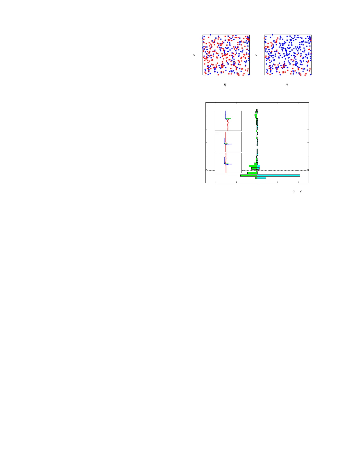
An Iterativ e Quadratic Method f or General-Sum Differ ential Games with F eedback Linearizable Dynamics David Fridovich-K eil*, V icenc ¸ Rubies-Royo*, and Claire J. T omlin Abstract — Iterative linear -quadratic (ILQ) methods are widely used in the nonlinear optimal control community . Recent work has applied similar methodology in the setting of multi- player general-sum differential games. Here, ILQ methods are capable of finding local equilibria in interactive motion planning problems in real-time. As in most iterative procedur es, however , this approach can be sensitiv e to initial conditions and hy- perparameter choices, which can result in poor computational performance or even unsafe trajectories. In this paper , we focus our attention on a br oad class of dynamical systems which are feedback linearizable, and exploit this structure to impro ve both algorithmic reliability and runtime. W e showcase our new algorithm in three distinct traffic scenarios, and observe that in practice our method con verges significantly more often and more quickly than was possible without exploiting the feedback linearizable structure. I . I N T RO D U C T I O N In robotics, a wide v ariety of decision making prob- lems, including lo w-lev el control, motion planning, and task planning, are often best expressed as optimal control problems. Specific algorithms and solution strategies may differ depending upon f actors such as system dynamics and cost structure; yet, modern methods such as model predictiv e control ha ve proven extremely effecti ve in many applications of interest. Still, optimal control formulations are fundamentally limited to solving decision problems for a single agent . Dynamic game theory—the study of games played over time—provides a natural e xtension of optimal control to the multi-agent setting. For example, nearby vehicles at an intersection (e.g., Fig. 1) mutually influence one another as they attempt to balance making forward progress in a de- sired direction while a voiding collision. Abstractly , dynamic games provide each agent, or “player, ” a separate input to the system, and allo w each player to hav e a different cost function which the y wish to optimize. Players may wish to cooperate with one another in some situations and not cooperate in others, leading to complicated, coupled optimal play . Moreover , dif ferent players may know different pieces of information at any point in time. Optimal play depends strongly upon this information structure; a player with an informational adv antage can often exploit that kno wledge to Department of EECS, UC Berkeley , { dfk, vrubies, tomlin } @eecs.berkeley.edu . ∗ indicates equal contribution. This research is supported by an NSF CAREER award, the Air Force Office of Scientific Research (AFOSR), NSF’ s CPS FORCES and V eHICaL projects, the UC-Philippine-California Advanced Research Institute, the ONR BRC grant for Multibody Systems Analysis, a DARP A Assured Autonomy grant, and the SRC CONIX Center . D. Fridovich-Keil is also supported by an NSF Graduate Research Fello wship. -20 -15 -10 -5 0 5 10 15 20 -20 0 20 40 60 80 100 120 140 -50 -40 -30 -20 -10 0 10 20 30 40 50 -40 -30 -20 -10 0 10 20 30 40 -40 -20 0 20 40 60 -30 -20 -10 0 10 20 30 40 50 60 (a) (b) (c) Fig. 1: Three traffic scenarios—(a) intersection, (b) high speed overtaking, and (c) roundabout merging—which we formulate as differential games and use to benchmark the performance of our method and a baseline [1]. the detriment of any competitors. For example, in poker a player who cheats and looks at the top card in the deck is more certain of who will win the next hand, and hence can assume less risk in betting. In this paper, we consider dynamic games played in con- tinuous time, or differential games. Historically , dif ferential games were first studied in zero-sum (perfectly competitiv e) settings such as pursuit-ev asion problems [2]. Here, optimal play is described by the Hamilton-Jacobi-Isaacs (HJI) PDE, in which the Hamiltonian includes a minimax optimization problem that encodes the instantaneous preferences of both players. These results extend to general-sum games as well, in which optimal play follows coupled HJ equations [3, 4]. Unfortunately , numerical solutions to these coupled PDEs often prove intractable because they operate on a densely discretized state space. Approximate dynamic programming methods [5] of fer a promising alternativ e; still, computational efficienc y remains a significant challenge. Recently , the robotics community has shown rene wed interest in dynamic and differential games [6–8], with a variety of ne w approximate algorithms for identifying locally optimal play . For example, Sadigh et al. [9] optimize the be- havior of a self-dri ving car while accounting for the reaction of a human driver . W ang et al. [10] demonstrate a real-time iterativ e best response algorithm for planning competitiv e trajectories in a 6-player drone racing game. Building upon the earlier sequential linear-quadratic method of [11] and the well-known iterativ e linear-quadratic regulator [12, 13], our own prior work [1] solves warm-started 3-player differential games in under 50 ms each, operating single-threaded on a consumer laptop. In this paper , we extend and improv e upon our pre vious work [1] by exploiting the structure in a broad class of dynamical systems. Many systems, including quadcopters and the planar unicycle and bicycle models commonly used to model automobiles, are feedback linearizable. That is, there exists a (nonlinear) control la w which renders the closed-loop input-output dynamics of these nonlinear sys- tems linear . Here, we dev elop an algorithm for identifying locally optimal play in differential games with feedback linearizable dynamics. W e establish theoretical equiv alence between the solutions identified using this algorithm and those which do not exploit the feedback linearizable struc- ture. By exploiting the structure, howe ver , our algorithm is able to tak e much lar ger steps at each iteration and generally con v erge to an equilibrium more quickly and more reliably than was previously possible. Experimental results in Section VI confirm these computational adv antages for the interactive traf fic scenarios shown in Fig. 1. I I . R E L A T E D W O R K T o put our work in context, here we provide a brief sum- mary of iterati ve linear-quadratic (ILQ) methods of solving differential games, other approximate techniques of solving games, and common ways in which feedback linearization is used to accelerate motion planning. A. ILQ methods and other appr oximate techniques Iterativ e linear-quadratic (ILQ) methods are increasingly popular in the nonlinear model predictive control (MPC) and motion planning communities [12, 14]. These algorithms refine an initial control law at each iteration by forming a Jacobian linearization of system dynamics and a quadratic approximation of cost, and solving the resulting LQR sub- problem. Because LQ games also offer an efficient solution, this approach has also been applied in the context of two- player zero-sum differential games by [11] and recently extended in [1] to the N -player general-sum setting. ILQ methods are local . For optimal control problems, this means that they generally con v erge to local optima; for differential games, if they con ver ge, they conv erge to local equilia. Im- portantly , these methods scale favorably with state dimension (cubic), number of players (cubic), and time horizon (linear), and [1] reports real-time operation for sev eral three-player examples. Iterativ e best response (IBR) algorithms comprise another class of methods for solving games. Here, in each iteration players sequentially solve (or approximately solve) the op- timal control problem which results when all other players’ strategies are fixed. IBR has been demonstrated in a wide variety of settings, including congestion games [15], drone racing [10], and autonomous dri ving [16]. As in the case of ILQ methods, con vergence is not generally guaranteed for arbitrary initializations. At best, IBR con ver ges to local Nash equilibria (e.g., [10]). Howe ver , by reducing the game to a sequence of optimal control problems, IBR algorithms can take advantage of existing MPC and planning tools. B. F eedback linearization in motion planning Feedback linearization is a popular differential geometric control technique which renders a class of nonlinear systems’ input-output response linear . W e provide a brief technical ov erview of feedback linearization in Section IV; here, we summarize its relev ance to motion planning. One of the early successes of feedback linearization was its effecti v eness in planning for chained systems, e.g., a car with multiple trailers [17, 18]. Feedback linearization (and the related notion of differential flatness) is also commonly used for minimum snap control of quadrotors [19, 20]. Here, the differentially flat structure of the underlying system dynamics allows planners to generate piece wise polynomial trajectories which the system can track exactly . This concept is extended to the case of differential games in [10], where each iteration of IBR yields a new spline trajectory . I I I . P RO B L E M F O R M U L AT I O N W e consider N -player , general-sum dif ferential games with control-affine dynamics. That is, we presume that the game state x ∈ R n ev olv es as ˙ x = f ( x ) + N X i =1 g i ( x ) u i , (1) where u i ∈ R k i is the control input of player i . In our examples (Section VI), x will be the concatenated states of multiple subsystems, but this is not strictly necessary . W e assume that (1) is full-state feedback linearizable, i.e. there exist outputs y = h ( x ) such that y and finitely many of its time deri vati v es e v olve linearly as a function of some auxiliary inputs z i ∈ R k i , for some control law u i := u i ( x, z i ) . A brief revie w of feedback linearization may be found in Section IV. Next, we suppose that each player i wishes to minimize a running cost ` i ov er finite time horizon T : J i ( u 1 , . . . , u N ) := Z T 0 ` i ( t, x, u 1 , . . . , u N ) dt . (2) W e shall require ` i to be C 2 in x, u j , ∀ j , uniformly in time t . Player i ’ s total cost J i then depends explicitly upon each player’ s control input signal u i ( · ) and implicitly upon the initial condition x (0) . Finally , we presume that each player i has access to the state x at every time t , but not other players’ control inputs u j , j 6 = i , i.e. u i ( t ) ≡ γ i  t, x ( t )  (3) for some measurable function γ i : [0 , T ] × R n → R k i . W e shall denote the set of such functions Γ i . For clarity , we shall also ov erload the notation of costs J i ( γ 1 ; . . . ; γ N ) ≡ J i  γ 1 ( · , x ( · )) , . . . , γ N ( · , x ( · ))  . Thus equipped with dynamics (1), costs (2), and informa- tion pattern (3), in principle, we seek Nash equilibria of the game. Definition 1: (Nash equilibrium, [21, Chapter 6]) A set of strategies ( γ ∗ 1 , . . . , γ ∗ N ) constitute a Nash equilibrium if no player has a unilateral incentiv e to deviate from his or her strategy . Precisely , the follo wing inequality must hold for each player i : J ∗ i ≡ J i ( γ ∗ 1 , . . . , γ ∗ i − 1 , γ ∗ i , γ ∗ i +1 , . . . , γ ∗ N ) ≤ J i ( γ ∗ 1 , . . . , γ ∗ i − 1 , γ i , γ ∗ i +1 , . . . , γ ∗ N ) , ∀ γ i ∈ Γ i . In practice, we may only be able to check if these con- ditions are satisfied locally in the neighborhood of strategy γ ∗ i , i.e., find local Nash equilibrium. As noted in [1] ILQ methods for games are known not to find ev en local Nash equilibria, b ut still be competiti ve and, importantly , efficient to compute. I V . B A C K G RO U N D : F E E D BA C K L I N E A R I Z A T I O N This section pro vides a brief re vie w of feedback lineariza- tion, a geometric control technique popularly used across a wide range of robotic applications including manipulation, quadrotor flight, and autonomous driving. Recall dynamics (1), and define the matrix g ( x ) := [ g 1 ( x ) , . . . , g N ( x )] ∈ R n × k and v ector u T = [ u T 1 , . . . , u T N ] ∈ R k , with k = P i k i the total control dimension. Thus, (1) may be rewritten as ˙ x = f ( x ) + g ( x ) u, y = h ( x ) (4) where y is the output of the system, and the functions f , g , and h are sufficiently smooth. A. Mechanics Suppose that (4) has well-defined vector relativ e degree ( r 1 , . . . , r k ) [22, Definition 9.15] and is full-state feedback linearizable. Then, there exists a matrix M ( x ) and vector m ( x ) such that the time deriv ati ves of the outputs y follow [ y ( r 1 ) 1 , . . . , y ( r k ) k ] T = M ( x ) u + m ( x ) . (5) Presuming the in vertibility of the so-called “decoupling matrix” M ( x ) , we may design the following feedback lin- earizing control la w as a function of both state x and an auxiliary input z ∈ R k : u ( x, z ) = M − 1 ( x )( z − m ( x )) , (6) which renders the input-output dynamics linear in the new auxiliary inputs z : [ y ( r 1 ) 1 , . . . , y ( r k ) k ] T = z . (7) Note that, as for u in (1) we shall consider z T = [ z T 1 , . . . , z T N ] to be a concatenation of auxiliary inputs for each player, with z i ∈ R k i . B. Change of coor dinates W e have seen how a careful choice of feedback linearizing controller u ( x, z ) renders the dynamics of the output y and its deriv ati ves linear . Define the state of this linear system as ξ := [ y 1 , . . . , y ( r 1 − 1) 1 , . . . , y k , . . . , y ( r k − 1) k ] T . Just as there is a bijectiv e map (6) between control u and auxiliary input z whene ver M ( x ) is in v ertible, there is also a bijection between state x and linear system state ξ , x = λ ( ξ ) [22] because (4) is full-state feedback linearizable. W e shall use both bijective maps (and their deriv ativ es) in Section V to rewrite costs (2) in terms of the linearized dynamics (7). V . M E T H O D S In this section we present our main contribution, a compu- tationally stable and efficient algorithm for identifying local equilibria of general-sum games with feedback linearizable dynamics. W e be gin in Section V -A by computing a feedback linearizing controller for unicycle dynamics, which we shall use as a running example throughout the paper . Then, in Section V -B we show how to transform the costs for each player to depend upon linear system state ξ and auxiliary inputs z i rather than state x and controls u i . In Section V -C we introduce the main algorithm, and finally in Section V -D we summarize the effects of using feedback linearization. A. F eedback linearization by example Consider the follo wing (single player) 4D unicycle dy- namical model: ˙ x =     ˙ p x ˙ p y ˙ θ ˙ v     =     v cos θ v sin θ w a     , y =  p x p y  (8) representing the ev olution of the positions p x and p y , the orientation θ , and speed v . The inputs w and a represent the angular rate and the acceleration. By taking time deri v ativ es of the output y follo wing the procedure from Section IV, we obtain the new set of states ξ = [ p x , ˙ p x , p y , ˙ p y ] T for the linearized system. Differentiation re veals that  ¨ p x ¨ p y  =  − v sin θ cos θ v cos θ sin θ   w a  . (9) From this result, we compute the in verse decoupling matrix and drift term as M − 1 ( x ) =  − sin θ/v cos θ /v cos θ sin θ  , m ( x ) = 0 . (10) Finally , we can also e xplicitly deri v e the state con v ersion map λ ( ξ ) λ ( ξ ) =      p x p y q ˙ p 2 x + ˙ p 2 y tan − 1 ( ˙ p y ˙ p x )      . (11) Now , consider a differential game with two players, each of whom independently follows dynamics (8). The in verse decoupling matrix M − 1 ( x ) and the Jacobian of the state con version map λ for the full system will be block diagonal. B. T r ansforming costs So far , we have introduced feedback linearization and shown ho w to deri ve the mappings from auxiliary input z to control u and linearized system state ξ to state x . T o exploit the feedback linearizable structure of (4) when solving the game, we must rewrite running costs ` i ( t, x, u 1 , . . . , u N ) in terms of ξ and z . Overloading notation, we shall denote the transformed running costs as ` i ( t ; ξ ; z 1 ; . . . ; z N ) ≡ ` i  t ; λ ( ξ ); u 1  λ ( ξ ) , z 1  ; . . . ; u N  λ ( ξ ) , z N   , (12) Algorithm 1: Feedback Linearized Iterative LQ Games Input: initial linearized system state ξ (0) and control strategies { γ 0 i } i ∈{ 1 ,...,N } , time horizon T Output: conv er ged control strategies { γ ∗ i } i ∈{ 1 ,...,N } for the linearized system 1 for iteration p = 1 , 2 , . . . do 2 µ p ≡ { ˆ ξ ( t ) , ˆ z i ( t ) } i ∈{ 1 ,...,N } ,t ∈ [0 ,T ] ← 3 getT rajectory  ξ (0) , { γ p − 1 i }  ; 4 { l i ( t ) , Q i ( t ) , R ij ( t ) } ← quadraticizeCost  µ p  ; 5 { ˜ γ p i } ← solveLQGame  { l i ( t ) , Q i ( t ) , R ij ( t ) }  ; 6 { γ p i } ← stepT ow ard  { γ p − 1 i , ˜ γ p i }  ; 7 if conver ged then 8 retur n { γ p i } where u i ( λ ( ξ ) , z i ) is giv en in (6). Section V -C presents our main algorithm; a core step will be to compute first and second deriv ativ es of each player’ s running cost with respect to the ne w state ξ and inputs z i . This may be done efficiently using the chain rule and exploiting known sparsity patterns for particular systems and costs. For completeness, howe v er , we shall ignore sparsity and illustrate computing the first deri v ati ve of ` i with respect to the j th dimension of ξ , denoted ξ j : ∂ ` i ∂ ξ j = n X p =1 ∂ ` i ∂ x p ∂ x p ∂ ξ j + N X n =1 k n X p =1 ∂ ` i ∂ u n,p n X q =1 ∂ u n,p ∂ x q ∂ x q ∂ ξ j (13) where u n,p is the p th entry of the n th player’ s control input. Second deriv ati ves may be computed similarly , though again we stress that for specific dynamics and cost functions it is often much more ef ficient to exploit the a priori known sparsity of partial deriv ati ves. Interestingly , we also observe that the terms arising from the second sum in (13), which account for the state-dependence of the feedback linearizing controllers (6), are often negligible in practice and may be dropped without significant impact on solution quality . C. Cor e algorithm Like the original iterative LQ game algorithm, we proceed from a set of initial strategies γ i for each player—understood now to map from ( t, ξ ) to z i —and iterativ ely refine them by solving LQ approximations. Our main contrib ution, there- fore, lies in the transformation of the game itself into the coordinates ξ , z i which correspond to feedback linearized dynamics. As we shall see in Section VI, iterati ve LQ approximations are much more stable in the transformed coordinates and con ver ge at least as quickly . Algorithm 1 outlines the major steps in the resulting algorithm. W e begin at the giv en initial condition ξ (0) for the linearized system and strategies γ 0 i for each player . Note that these strategies define control laws for the linearized system , i.e. z i ( t ) ≡ γ i  t, ξ ( t )  . At each iteration, we first (Algorithm 1, line 3) integrate the linearized dynamics (7) forward to obtain the current operating point ( ˆ ξ ( · ) , { ˆ z i ( · ) } ) . Then (Algorithm 1, line 4), we compute a quadratic approximation to each player’ s running cost in terms of the variations δξ := ξ − ˆ ξ and δ z j := z j − ˆ z j ` i ( t ; ξ ; z 1 ; . . . ; z N ) − ` i ( t ; ˆ ξ ; ˆ z 1 ; . . . ; ˆ z N ) ≈ δ ξ T l i ( t )+ 1 2 δ ξ T Q i ( t ) δ ξ + 1 2 N X j =1 δ z T j ( R ij ( t ) δ z j + 2 r ij ( t )) , (14) using the chain rule as in (13) to compute the terms l i , Q i and R ij for each player . Equipped with linear dynamics (7) and quadratic costs (14), the solution of the resulting general-sum LQ game is giv en by a set of coupled Riccati differential equations, which may be derived from the first order necessary condi- tions of optimality for each player [21, Chapter 6]. In practice (Algorithm 1, line 5), we numerically solve these equations in discrete-time using a time step of ∆ t . If a solution exists at the p th iteration, it is known to take the form ˜ γ p i ( t, ξ ) ≡ ˆ z i ( t ) − P p i ( t )  ξ ( t ) − ˆ ξ ( t )  − α p i ( t ) (15) for matrix P p i ( t ) and vector α p i ( t ) [21, Corollary 6.1]. W e cannot simply use these strategies at the ( p + 1) th iteration or we risk div erging, howe ver , without further as- sumptions on the curv ature and con v exity of running costs ` i . In fact, these costs are generally noncon ve x when expressed in terms of ξ and z j (12), which necessitates some care in updating strategies. T o address this issue (Algorithm 1, line 6), we follow a common practice in the ILQR and sequential quadratic programming literature (e.g., [23]) and introduce a step size parameter η ∈ (0 , 1] : γ p i ( t, ξ ) = ˆ z i ( t ) − P p i ( t )  ξ ( t ) − ˆ ξ ( t )  − η α p i ( t ) . (16) Observe that, taking η = 0 and recalling that ξ (0) = ˆ ξ (0) , we recov er the previous open-loop control signal γ p i ( t, ξ ) = ˆ z i , ∀ t ∈ [0 , T ] . T aking η = 1 , we recover the LQ solution from this iteration (15). As is common in the literature, we perform a backtracking linesearch on η , starting with initial value η 0 and terminating when the trajectory that results from (16) satisfies a trust region constraint at le vel  . In our experiments, we use an L ∞ constraint, i.e. k ξ ( t ) − ˆ ξ ( t ) k ∞ < , ∀ t, (17) and check that M − 1 exists at each time. D. Effect of feedback linearization In comparison to the non-feedback linearizable case, the linearized dynamics (7) are independent of trajectory (and hence also of iteration). That is, in the non-feedback lineariz- able case [1], each iteration be gins by constructing a Jacobian linearization of dynamics (1); this is superfluous in our case. As a consequence, lar ge changes in auxiliary input z between iterations—which lead to lar ge changes in state trajectory— are trivially consistent with the feedback linearized dynamics (7). By contrast, a large change in control u may take the nonlinear dynamics (1) far aw ay from the pre vious Jacobian linearization, which causes the algorithm from [1] to be fairly sensitiv e to step size η and trust region size  . W e study this sensitivity more carefully in Section VI. Finally , it is important to note that while many sys- tems of interest (e.g., manipulators, cars, and quadrotors) are feedback linearizable, this is not true of all systems. Additionally , there are two drawbacks of our algorithm that deserve mention. First, we must take care to avoid regions in which M − 1 does not exist. W e accomplish this by designing costs that penalize proximity to singularities. While this can potentially limit the range of behaviors, man y motion problems naturally incorporate these costs. Second, the transformed costs ` i ( t ; ξ ; . . . ) may ha ve much more varied, extreme curvature than the original costs ` i ( t, x, . . . ) . In some cases, this can make Algorithm 1 sensitive to linesearch parameters η 0 and  , even of fsetting the benefits mentioned abo ve. W e defer further discussion and empirical study for Section VI. V I . R E S U L T S In this section, we study the empirical performance of Algorithm 1. In Section VI-A, we quantify the improv ements in algorithmic stability from Section V -D for an intersection scenario. In Section VI-B, we discuss a case in which the e xtreme curvature of the transformed cost ` i ( t ; ξ ; . . . ) alluded to also in Section V -D which causes Algorithm 1 to con v erge v ery slo wly . In practice, howe ver , this is not necessarily a serious problem. In Section VI-C, we redesign this problematic cost function to depend explicitly upon ξ rather than x without changing the semantic character of equilibria. A. Impr ovements in solver stability T o showcase the benefits of our feedback linearization- based approach, we study the empirical sensiti vity of so- lutions to the initial step size η 0 and trust region size  hyperparameters from Section V -C. W e shall consider a three-player intersection example and compare the strategies identified by Algorithm 1 with those identified on the original dynamics, using the algorithm from [1]. Here, two cars, modeled with bicycle dynamics   ˙ p x ˙ p y ˙ θ   =   v cos θ v sin θ ( v /L ) tan φ   ,   ˙ v ˙ φ ˙ a   =   a ω κ   (18) (with inter -axle distance L and inputs ω controlling front wheel rate ˙ φ and κ controlling jerk), and a pedestrian modeled with dynamics (8) navigate an intersection. Like (8), bicycle dynamics (18) are feedback linearizable in the out- puts ( p x , p y ) . W e place quadratic penalties on each player’ s distance from the appropriate lane center and from a fixed goal location, as well as on the difference between speed v and a fixed nominal speed ¯ v . Players are also penalized quadratically within a fixed distance of one another 1 . 1 For details concerning weighing of different cost terms we re- fer the reader to our github repository at https://github.com/ HJReachability/ilqgames 0.2 0.4 0.6 0 2 4 6 8 10 Ours 0.2 0.4 0.6 0 2 4 6 8 10 Baseline Fig. 2: Distribution of pairs ( η 0 ,  ) colored by quality metric q . Pairs with low q are colored blue, and high q pairs are colored red. - 200 - 100 0 100 200 Number of trajectories (sampled uniformly in 0 , ) 0 10 20 30 40 50 60 Similarity to desired (x,y) trajectory Baseline Ours A B C B A C D D q* Fig. 3: Comparison of the proposed algorithm with the state of the art [1] for a three player intersection game. Histograms (left, baseline; right, ours) show that our method is much more numerically stable and conv erges more frequently . Insets labelled { A, B, C, D } show a typical trajectory for the associated bin. The dotted horizontal line shows threshold q ∗ , used to distinguish samples from Fig. 2. In order to assess the quality of a trajectory µ = ( ξ , z 1 , . . . , z N ) generated by a particular algorithm, we define the similarity metric to the desired trajectory to be: q ( µ, ˜ µ ) := max t ∈ [0 ,T ] k ξ ( t ) − ˜ ξ ( t ) k 2 , ( p x ,p y ) . (19) Here, we take ˜ µ := ( ˜ ξ , ˜ z 1 , . . . , ˜ z N ) to be the equilibrium trajectory which that algorithm ideally conv erges to. The norm measures Euclidean distance only in the ( p x , p y ) dimensions. T rajectories that diver ge or con ver ge to unrea- sonable solutions yield high v alues for q , while trajectories that closely match ˜ µ incur low values. W e fix the initial conditions and cost weights identically for both algorithms. Thus, an y trajectory µ identified by the solver will solely be a function of the initial step size η 0 and trust region size  . Therefore, we will ov erload the penalty metric notation as q ( η 0 ;  ) . Given this metric we study the quality of solutions ov er the ranges η 0 ∈ [0 . 1 , 0 . 75] and  ∈ [1 . 0 , 10 . 0] , and test 324 uniformly sampled ( η 0 ,  ) pairs. Fig. 2 displays the sampled pairs ov er the space of η 0 and  . For clarity , we set a success threshold q ∗ and color “successful” pairs with q ( η 0 ;  ) ≤ q ∗ blue, and “unsucessful” pairs red. Fig. 3 shows histograms of solution quality q for each algorithm, with a horizontal line denoting thresh- old q ∗ . W e observe that solving the game using feedback linearization con ver ges much more reliably than solving it for the original nonlinear system. Moreover , for conv erged trajectories with low q -v alue, the av erage computation time was 0 . 3982 ± 0 . 3122 s (mean ± standard deviation) for our method and 0 . 8744 ± 0 . 9582 s for the baseline. B. Sensitivity to transformed cost landscape Unfortunately , these results do not generalize to all games. As per Section V -D, in some cases the cost landscape gets much more complicated when e xpressed in linearized system coordinates ξ , z i . For e xample, a simple quadratic penalty on a single player’ s speed difference from nominal ¯ v in (8) is noncon ve x and non-smooth near the origin when expressed as a function of linearized system state ξ : ( v − ¯ v ) 2 ⇐ ⇒  ¯ v − q ˙ p 2 x + ˙ p 2 y  2 . (20) Consequences vary; the ef fect is negligible in the intersection example from Fig. 3, b ut it is more significant in the roundabout example below in Section VI-C, where cars must slow do wn before turning into the roundabout. C. Designing costs directly for the linearized system Fortunately , in practical settings of interest it is typically straightforward to design smooth, semantically equiv alent costs e xplicitly as functions of the linearized system coordi- nates ξ . For e xample, we can replace the nominal speed cost of (20) with a time-varying quadratic penalty in that player’ s position ( p x , p y ) : ( v − ¯ v ) 2 = ⇒  p x ( t ) − ¯ p x ( t )  2 +  p y ( t ) − ¯ p y ( t )  2 , (21) where  ¯ p x ( · ) , ¯ p y ( · )  defines the point on the lane center a distance ¯ v t from the initial condition. W e demonstrate the effecti veness of this substitution in two examples—mer ging into a roundabout, and ov ertaking a lead vehicle—in which the original cost (20) led to instability in Algorithm 1. In both cases, we also use simple quadratic penalties for z i (rather than transforming k u i k 2 into lin- earized coordinates), albeit with dif ferent weightings. Results for the roundabout merging and overtaking examples are shown in Figures 4 and 5, respecti vely . From the 324 samples in each (drawn from expanded ranges η 0 ∈ [0 . 1 , 1 . 0] ,  ∈ [1 , 50] ), we see that Algorithm 1 con ver ged more frequently than the method of [1]. Moreov er , when successful, the av erage computational time in the roundabout example was 0 . 2797 ± 0 . 1274 s for our method and 0 . 4244 ± 0 . 5259 s for the baseline. Runtimes for the ov ertaking example were 0 . 5112 ± 0 . 3228 s (ours) and 0 . 4417 ± 0 . 4142 s (baseline). Observe how runtimes for our approach cluster more tightly around the mean, indicating a more reliable conv ergence rate. V I I . C O N C L U S I O N W e have presented a novel algorithm for identifying local equilibria in dif ferential games with feedback linearizable dynamics. Our method works by repeatedly solving LQ games in the linearized system coordinates, rather than in the original system coordinates. By working with the linearized system, our algorithm becomes less sensitiv e to parameters such as initial step size and trust region size, which often leads it to con ver ge faster . Our method is fully general, i.e. - 200 - 100 0 100 200 Number of trajectories (sampled uniformly in 0 , ) 0 5 10 15 20 25 30 35 40 45 50 Similarity to desired (x,y) trajectory Baseline Ours A B C D E C B A E D Fig. 4: Comparison for a roundabout merging example with four cars. - 100 - 50 0 50 100 Number of trajectories (sampled uniformly in 0 , ) 0 5 10 15 20 25 30 35 Similarity to desired (x,y) trajectory Baseline Ours A B C B A C Fig. 5: Comparison for a three vehicle high speed overtaking maneuver . any cost expressed in terms of nonlinear system coordinates may also be expressed in terms of linearized coordinates. Howe v er , in some cases transforming costs in this way makes the cost landscape extremely complicated. In such cases, it is often possible to design semantically equi valent replacement costs directly in the linearized coordinates. W e test our method in a variety of competiti ve traffic scenarios. Using appropriately redesigned costs when necessary , our ex- periments confirm the computational stability and ef ficiency of our approach. R E F E R E N C E S [1] D. Fridovich-Keil et al. “Efficient Iterative Linear- Quadratic Approximations for Nonlinear Multi-Player General-Sum Differential Games”. arXiv pr eprint arXiv:1909.04694 (2019). [2] R. Isaacs. Games of pursuit . T ech. rep. Rand Corpo- ration, 1951. [3] A. W . Starr and Y .-C. Ho. “Nonzero-sum dif ferential games”. Journal of Optimization Theory and Applica- tions 3.3 (1969). [4] A. Starr and Y .-C. Ho. “Further properties of nonzero- sum differential games”. Journal of Optimization The- ory and Applications 3.4 (1969). [5] D. P . Bertsekas and J. N. Tsitsiklis. Neuro-dynamic pr ogr amming . Athena Scientific Belmont, MA, 1996. [6] A. Drev es and M. Gerdts. “A generalized Nash equi- librium approach for optimal control problems of autonomous cars”. Optimal Contr ol Applications and Methods 39.1 (2018). [7] A. Dre ves. “A best-response approach for equilibrium selection in two-player generalized Nash equilibrium problems”. Optimization 68.12 (2019). [8] G. W illiams et al. “Best response model predicti ve control for agile interactions between autonomous ground vehicles”. 2018 IEEE International Confer- ence on Robotics and A utomation (ICRA) . IEEE. 2018. [9] D. Sadigh et al. “Planning for autonomous cars that lev erage ef fects on human actions.” Robotics: Science & Systems . Ann Arbor, MI, USA. 2016. [10] Z. W ang, R. Spica, and M. Schwager . “Game Theo- retic Motion Planning for Multi-robot Racing”. Dis- tributed A utonomous Robotic Systems . Springer, 2019. [11] H. Mukai et al. “Sequential linear quadratic method for differential games”. Pr oc. 2nd D ARP A-JF A CC Symposium on Advances in Enterprise Control . Cite- seer . 2000. [12] W . Li and E. T odoro v. “Iterative linear quadratic regulator design for nonlinear biological movement systems.” ICINCO . 2004. [13] D. H. Jacobson and D. Q. Mayne. “Differential dy- namic programming” (1970). [14] J. v an den Berg. “Iterated LQR smoothing for locally- optimal feedback control of systems with non-linear dynamics and non-quadratic cost”. American Contr ol Confer ence (ACC) . IEEE. 2014. [15] A. Jonsson and M. Rovatsos. “Scaling up multiagent planning: A best-response approach”. International Confer ence on Automated Planning and Scheduling . 2011. [16] M. W ang et al. “Game Theoretic Planning for Self- Driving Cars in Competitiv e Scenarios”. Robotics: Science & Systems . 2019. [17] R. M. Murray and S. S. Sastry . “Nonholonomic mo- tion planning: Steering using sinusoids”. T ransactions on Automatic Contr ol 38.5 (1993). [18] P . Rouchon et al. “Flatness, motion planning and trailer systems”. Conference on Decision and Contr ol (CDC) . V ol. 3. IEEE. 1993. [19] D. Mellinger and V . K umar . “Minimum snap trajectory generation and control for quadrotors”. International Confer ence on Robotics and Automation . IEEE. 2011. [20] C. Richter, A. Bry, and N. Roy. “Polynomial trajec- tory planning for aggressive quadrotor flight in dense indoor en vironments”. Robotics Researc h . Springer, 2016. [21] T . Bas ¸ ar and G. J. Olsder. Dynamic Noncooperative Game Theory . SIAM, 1999. [22] S. Sastry. Nonlinear Systems: Analysis, Stability , and Contr ol . Springer, 1999. [23] Y . T assa, N. Mansard, and E. T odoro v. “Control- limited dif ferential dynamic programming”. Inter- national Confer ence on Robotics and Automation (ICRA) . IEEE. 2014.