Learning to Fuse Music Genres with Generative Adversarial Dual Learning

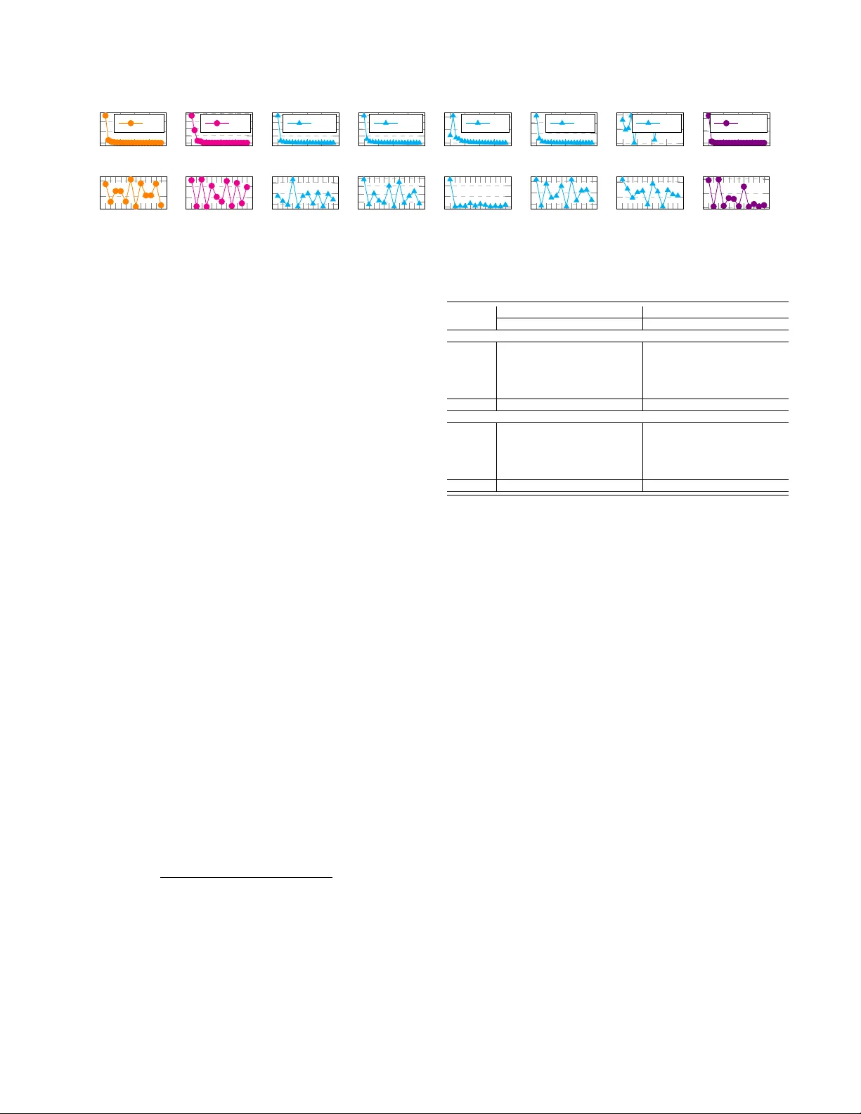
Learning to Fuse Music Genr es with Generativ e Adversarial Dual Learning Zhiqian Chen ∗ , Chih-W ei W u † , Y en-Cheng Lu ∗ , Alexander Lerch † and Chang-T ien Lu ∗ ∗ Computer Science Department, V ir ginia T ech Email: { czq,kevinlu,ctlu } @vt.edu † Center for Music T ec hnology , Geor gia Institute of T echnolo gy Email: { cwu307, alexander .ler ch } @gatech.edu Abstract —FusionGAN is a novel genre fusion framework for music generation that integrates the strengths of gener - ative adversarial networks and dual learning. In particular , the proposed method offers a dual learning extension that can effectively integrate the styles of the given domains. T o efficiently quantify the difference among diverse domains and av oid the vanishing gradient issue, FusionGAN provides a W asserstein based metric to approximate the distance between the target domain and the existing domains. Adopting the W asserstein distance, a new domain is created by combining the patterns of the existing domains using adversarial learning. Experimental results on public music datasets demonstrated that our approach could effectively merge two genres. I . I N T R O D U C T I O N Computational creativity is a liv ely research area that focuses on understanding and facilitating human creativity through the implementation of software programs [2]. W ith the rapid advances in data-driven algorithms such as deep learning [7], the exploration into computational creativity via machine learning approaches has become increasingly popular . Examples showing the potential of deep learning for creativ e approaches are the artistic style transfer on images [4] and videos [12]. Music, with its comple x hierarchical and sequential structure and its inherent emotional and aesthetic subjectivity , is an intriguing research subject at the core of human creativity . While there has been some work on generativ e models for music, research that in vestigates the capabilities of deep learning for creativ e applications such as style transfer is limited. This paper aims to fill this space by exploring the idea of style fusion in music with generative adversarial dual learning. In the field of unsupervised generative learning, genera- tiv e adversarial networks (GAN) [6] hav e recently gained considerable attention. It is important to note, howe ver , that GANs are designed to learn from a single domain and cannot discov er cross-domain knowledge. Inspired by dual learning in machine translation, sev eral recent publications propose methods to pair unlabeled data points in different domains by optimizing bi-directional reconstruction errors [14], [8], [16]. Although these methods are designed to address the challenge of multimodal learning, they do not address the problem of domain fusion. The goal of this paper is to provide a solution for fusing two or more groups of sequential patterns using unsupervised methods. Specifically , we focus on the problem of generating music with a fused music genre. T o combine genres using generative adversarial learning, we propose a framew ork for integrating multiple GANs. Unlike previous work, our study targets the creation of an unknown domain by mixing two given domains; a multi-way GAN-based model is proposed to absorb existing patterns and yield a new mixture. W ith the utilization of the W asserstein measure [1], we pose a distance constraint on the new domain that automatically balances its relation to the giv en domains. As a result, our model is capable of generating a mixed pattern after con ver gence. The main contributions of this paper are: • A novel framework for unsupervised music fusion : The dual learning scheme is e xtended to in volv e multi- ple domains by le veraging mutual regularization. In this way , the proposed framew ork enables the new domain to keep equal similarities with the giv en domains and produce a mixture of existing sequential patterns. • A sequence fusion method using GANs : T o apply unsupervised fusion learning, we extend the generativ e adversarial model so that multiple generators and dis- criminators can be updated by one another . • Formulation of an objective function indicating fu- sion progr ess : An objecti ve function based on W asser- stein distance is designed to integrate the information from multiple domains and represent learning progress. I I . R E L AT E D W O R K Music Genre Fusion: Fusion is mostly known as the sub-genre of jazz that emerged in the late ’60s, and that combines se veral musical styles such as funk, rock, and blues with the jazz harmony and improvisation [5]. The term can be generalized, howe ver , to any combinations of music genres. The creativ e combination of two or more genres obviously requires not only intimate kno wledge of the stylistic characteristics of the inv olved genres but also extensi ve compositional experience and skill to combine genres in a meaningful and satisfying way . Recently , Engel et al. [3] proposed a new approach of generating new musical sounds through interpolating the latent space learned by W av eNet [11] autoencoders. Additionally , Gatys et al. demonstrated the Deep Neural Networks’ (DNNs) capabili- ties of learning the artistic styles by blending the style of the training materials to the testing images using ConvNet [4]. Both examples show the great potential of using DNNs for merging two abstract concepts without the need for domain knowledge and explicitly defined rules. Cross-domain GAN: GAN [6], which has quickly risen to one of the most popular generative approaches, learns patterns without requiring adversarial e xamples or labels. In CGAN [10], the generator G has a conditional parameter c and will learn the conditional distribution of the data. Howe ver , those conditions need to be provided manually , somewhat similar to supervised learning. CoGAN [9] is proposed to learn a joint distribution with only samples drawn from the marginal distributions. DiscoGAN [8] solves the cross-domain pairing by minimizing bi-directional recon- struction loss, while DualGAN [14] takes advantage of the dual learning paradigm in machine translation. CycleGAN [16] presents a method whose mapping functions are cycle- consistent and proposes a cycle consistency loss function to further reduce the space of possible mapping functions. Different from the previous studies, our work raises a new problem, i.e., merging two sequential patterns into one. W e propose a GAN-based framework that merges two domains without manually tuning the distance between the given domains and the target domain. I I I . L E A R N I N G T O B L E N D M U S I C W I T H F U S I O N G A N A. Pr oblem Definition This paper aims to characterize music fusion across different genres in an unsupervised manner . Based on the data X A and X B from existing music domains D A , D B respectiv ely , our goal is to create a new domain D F which resembles both D A and D B . In the first phase, the ne w domain D F is expected to learn from D A , D B and keep an equal distance from both. Specifically , the generator G F of D F obtains feedback from the discriminators D A , D B of existing domains D A , D B , while the discriminator D F collects data from G F and D A , D B for iterativ e updating. The G F from the ne w domain minimizes the distance from the domains D A , D B , respectiv ely , and keeps the same distance from D A and D B . B. FusionGAN First, the framework initializes individual GAN models for existing domains. Maximum likelihood estimation using Long Short T erm Memory (LSTM) is applied to initialize the sequence generators G A ( G B ) . Then D A ( D B ) are trained giv en the domain data and sequence sampled from G A ( G B ) . Then GAN is employed to iterati vely enhance the G A ( G B ) and D A ( D B ). After pre-training, we build a GAN model for the new domain using the feedback from the models con- structed in the pre-training procedure. First, a new domain D F is initialized randomly and trained by both D A and D B . Follo wing the dual learning strategy , D A is enhanced by D B and D F in the second phase. Similarly , D B is improved by D A and D F . Such learning proceeds until conv ergence. The framew ork overvie w is shown in Figure 1. Figure 1: FusionGAN frame work In FusionGAN, we employ the W asserstein-1 distance for all discriminators because it is sensible when the learning distributions are supported by low dimensional manifolds [1]. T o av oid the intractable infimum in W asserstein-1 dis- tance, we resort to its Kantorovich-Rubinstein duality [13]: W ( P r , P θ ) = sup k f k L ≤ 1 E x ∼ P r [ f ( x )] − E x ∼ P θ [ f ( x )] . For the vanilla GAN, the goal is to find the optimal configuration of the parameters φ of discriminator ( f = D ). When the discriminator is optimized, the maximized W asserstein distance can be used as rew ard in the policy gradient process of the generator . Similarly , we define a three-way W asserstein distance as the objecti ve function: W ( P X A , P X B , P θ ) = L to measure the integrated distance between P θ and P X A , P X B . This measure should consider the relationship between e very pair of domains. The frame- work consists of three pairs of generators and discriminators, i.e., G A − D A , G B − D B , G F − D F , and two input data, i.e., X A , X B . For each discriminator , there are fiv e possible inputs, i.e., X A , X B , G A , G B , G F . Collecting all possible inputs w .r .t. the three discriminators, the objective function to maximize is defined as: L = W  P X A , P X B , P θ  E x ∼ P X A [ D A ( x )] − E x ∼ P X B [ D A ( x )] − E z ∼ p ( z ) [ D A ( G A ( z ))] − E z ∼ p ( z ) [ D A ( G B ( z ))] − E z ∼ p ( z ) [ D A ( G F ( z ))] − E x ∼ P X A [ D B ( x )] + E x ∼ P X B [ D B ( x )] − E z ∼ p ( z ) [ D B ( G A ( z ))] − E z ∼ p ( z ) [ D B ( G B ( z ))] − E z ∼ p ( z ) [ D B ( G F ( z ))] + E x ∼ P X A [ D F ( x )] + E x ∼ P X B [ D F ( x )] + E z ∼ p ( z ) [ D F ( G A ( z ))] + E z ∼ p ( z ) [ D F ( G B ( z ))] − E z ∼ p ( z ) [ D F ( G F ( z ))] , (1) where the first five terms are for D A , the second five terms are for D B , and the last five terms are for D F . This loss is used to update all the generators and discriminators. The following two subsections, III-C and III-D, will present the update rules using Eq. 1. C. D F Update of FusionGAN Removing the terms that are unrelated to D F in Eq. 1 (zero deri vati ve w .r .t. D F and G F ), we have the objectiv e function for updating D F and G F : L F = E x ∼ P X A [ D F ( x )] + E x ∼ P X B [ D F ( x )] + E z ∼ p ( z ) [ D F ( G A ( z ))] + E z ∼ p ( z ) [ D F ( G B ( z ))] − E z ∼ p ( z ) [ D F ( G F ( z ))] − E z ∼ p ( z ) [ D A ( G F ( z ))] − E z ∼ p ( z ) [ D B ( G F ( z ))] . (2) First, L F is calculated w .r .t. G F so as to update G F . Consid- ering dif ferentiating ∇ θ L F , the optimal G F is approximated as its con vergence. The proof is provided below to show that this deriv ative is principled under the optimality assumption. Theorem III.1 (FusionGAN Optimality Theorem) . Let P X A and P X B be any distribution, Let P θ be the distribution of G F θ ( Z ) with Z , a random variable with density p and G F θ a function satisfying E z ∼ p [ L ( θ , z )] < + ∞ , where L is Lipschitz constants. All functions are well-defined. Then ther e is a solution D F : X → R to the problem: W  P X A , P X B , P θ  = max k D F k L ≤ 1 L F . (3) and we have: ∇ θ L G F = ∇ θ W  P X A , P X B , P θ  = − E z ∼ p ( z ) ∇ θ X i ∈{ A,B ,F } D i ( G F ( z )) (4) Pr oof of Theor em III.1: Let us define L F = V ( ˜ D F , θ ) where ˜ D F lies in F = { ˜ D F : X → R , ˜ D F ∈ C b ( X ) , k D F k L ≤ 1 } and θ ∈ R d . By the Kantorovich- Rubinstein duality , there is an f ∈ F that satisfies: W  P X A , P X B , P θ  = sup ˜ D F ∈F V ( ˜ D F , θ ) = V ( D F , θ ) . Let us define X ∗ ( θ ) = { D F ∈ F : V ( D F , θ ) = W ( P X A , P X B , P θ ) } , which shows that X ∗ ( θ ) is non-empty . According to Theorem 1 in [1]: (1) if G F is continuous in θ , so is W ( P X A , P X B , P θ ) , (2) If G F is locally Lipschitz and satisfies E z ∼ p [ L ( θ , z )] < + ∞ , then W ( P X A , P X B , P θ ) is continuous and differentiable for any D F ∈ X ∗ ( θ ) when both terms are well-defined. Let D F ∈ X ∗ ( θ ) , which we knows exists since X ∗ ( θ ) is non-empty for all θ . Then: ∇ θ W  P X A , P X B , P θ  = ∇ θ V ( D F , θ ) = ∇ θ L F = − ∇ θ E z ∼ p ( z ) [ D F ( G F ( z )) + D A ( G F ( z )) + D B ( G F ( z ))] , (5) since D F is 1-Lipschitz. Furthermore, G F θ ( z ) is locally Lip- schitz as a function of ( θ , z ). Therefore, G F θ ( z ) is locally Lipschitz on ( θ , z ) with constants L ( θ , z ) . By Radamach- ers Theorem, D F ( G F θ ( z )) has to be differentiable almost ev erywhere for ( θ , z ) jointly . Re writing this, the set A = { ( θ , z ) : D F ◦ G F is not differentiable } has measure 0. By Fubinis Theorem, this implies that for almost ev ery θ the section A θ = { z : ( θ , z ) ∈ A } has measure 0. Let’ s fix a θ 0 such that the measure of A θ 0 is null. For this θ 0 we have ∇ θ D F ( G F θ ( z )) | θ 0 is well-defined for almost any z , and since p ( z ) has a density , it is defined p ( z ) almost ev erywhere. Giv en the condition E z ∼ p [ L ( θ , z )] < + ∞ , we hav e E z ∼ p ( z ) [ k∇ θ D F ( G F θ ( z )) k ] ≤ E z ∼ p ( z ) [ L ( θ 0 , z )] < + ∞ , (6) so E z ∼ p ( z ) [ ∇ θ f ( g θ ( z ))] is well-defined for almost e very θ 0 . T o keep the notation simple, we lea ve it implicit in the following equation that the E subjects to z ∼ p ( z ) . : 1 k θ − θ 0 k X i  E [ D i ( G F θ ( z ))] − E [ D i ( G F θ 0 ( z ))] − h ( θ − θ 0 ) , E [ ∇ θ [ D i ( G F θ ( z ))]] | θ 0 i  = 1 k θ − θ 0 k X i E  D i ( G F θ ( z )) − D i ( G F θ 0 ( z )) − h ( θ − θ 0 ) , ∇ θ [ D i ( G F θ ( z ))] | θ 0 i  ≤ 1 k θ − θ 0 k X i   k θ − θ 0 k L ( θ 0 , z ) + k θ − θ 0 k · k∇ θ [ D i ( G F θ ( z ))]   ≤ X i 2 L ( θ 0 , z ) = 6 L ( θ 0 , z ) , (7) where i ∈ { A, B , F } . By differentiability , the term inside the integral con verges p ( z ) to 0 as θ → θ 0 . Furthermore, and since E z ∼ p ( z ) [6 L ( θ 0 , z )] < + ∞ , we get by dominated con ver gence that Eq. 5 con verges to 0 as θ → θ 0 . So the result of Eq. 5 equals to: − E z ∼ p ( z ) [ ∇ θ D F ( G F ( z )) + ∇ θ D A ( G F ( z )) + ∇ θ D B ( G F ( z ))] . Therefore, the update rules for the parameters θ of G F is Eq. 4. Figure 2: FusionGAN: update G F The physical meaning is that all three discriminators can offer feedback to generator G F as sho wn in Fig. 2. The left cyan rectangle indicates D A , the middle pink one is D F , and the right yellow one D B . Similarly , the gradient w .r .t. the parameters φ of D F is: ∇ φ L F = ∇ φ  E x ∼ P X A [ D F ( x )] + E x ∼ P X B [ D F ( x )] + E z ∼ p ( z ) [ D F ( G A ( z ))] + E z ∼ p ( z ) [ D F ( G B ( z ))] − E z ∼ p ( z ) [ D F ( G F ( z ))]  . (8) Figure 3: FusionGAN: update D F As sho wn in Fig. 3, the update for D F actually implicitly balances itself between D A and D B . Howe ver , this update does not cover the degree of blending which may lead to an unbalanced mixture. Specifically , a good learning process for the discriminator D F should consider two factors: (1) minimizing the distance with D A , D B and D F simultane- ously and (2) maintaining a equal distance from D A and D B so as to satisfy both domains. T o satisfy (2) and push the discriminator D F to have a well-proportioned blending, an additional constraint is employed to further balance the ratio of existing domains, i.e., D A , D B : L F − bal =   E z ∼ p ( z ) [ D F ( G A ( z ))] − E z ∼ p ( z ) [ D F ( G B ( z ))]   +    E x ∼ P X A [ D F ( x )] − E x ∼ P X B [ D F ( x )]    . (9) D. D A and D B Update of FusionGAN After updating D F , FusionGAN will improve D A and D B . Since D A and D B are symmetric in the framew ork, we only discuss D A as shown in Fig. 9. Keeping related terms in Eq. 1, we get the loss function for D A : L A = E x ∼ P X A [ D A ( x )] − E x ∼ P X B [ D A ( x )] − E z ∼ p ( z ) [ D A ( G A ( z ))] − E z ∼ p ( z ) [ D A ( G B ( z ))] − E z ∼ p ( z ) [ D A ( G F ( z ))] − E z ∼ p ( z ) [ D B ( G A ( z ))] + E z ∼ p ( z ) [ D F ( G A ( z ))] . (10) T aking the deriv ati ve of L A w .r .t. D A , we hav e ∇ D A L A = ∇ D A  E x ∼ P X A [ D A ( x )] − E x ∼ P X B [ D A ( x )] − E z ∼ p ( z ) [ D A ( G A ( z ))] − E z ∼ p ( z ) [ D A ( G B ( z ))] − E z ∼ p ( z ) [ D A ( G F ( z ))]  . (11) Figure 4: FusionGAN: update D A There are four negativ e terms and one positive term in Eq. 11 w .r .t. D A . The training implicitly increases the positiv e terms and decreases the value of the negati ve terms. How- ev er , the inequalities in the two groups are not controlled. T o further control the distance among the three domains, we propose an inequality constraint for D A : D A ( X A ) ≥ D A ( G F ( z )) ≥ D A ( X B ) (12) Then combining Eq. 12 into loss function Eq. 11, it can be rewritten as: L A − bal = k D A ( X A ) − D A ( G F ( z )) k + k D A ( G F ( z )) − D A ( X B ) k . (13) Figure 5: FusionGAN: update G A Some inequalities that have been implicitly included in GAN training are not covered in Eq. 12, such as D A ( X A ) ≥ D A ( G A ) . Similar to the G F update in Fig. 5, the deri vati ve of L A w .r .t. G A is: ∇ G A L A = E z ∼ p ( z ) ∇ G A  − D A ( G A ( z )) − D B ( G A ( z )) + D F ( G A ( z ))  . (14) E. Algorithm Description The Algorithm 1 1 initializes the parameters of the discrim- inators and generators (line 1). T extCNN [15] and LSTM are employed to build the discriminators and generators respectiv ely . Gi ven X A , the generator is updated by maxi- mum likelihood estimation (line 3). From lines 4 to 5, D A receiv es the sequences generated by G A as negati ve data, and real data as positive samples. Between lines 6 and 16, a GAN procedure is applied to optimize D A and G A . D A returns regression scores that are treated as rewards for the policy gradient of G A . Similarly , D A improv es itself by the real world data X A and the data generated by G A . Our method proceeds to update D B and G B by using the same process from lines 3 to 16. D F repeats the same pre-training procedure from 3 to 16 with D F , G F , X F = X A + X B . From line 21 to 28, the framework iterativ ely updates the generators and discriminators from D F , D A , D B . Lines 21 to 24 are for D F , while lines 25 to 28 are for D A and D B . The update rules for the parameters of D F and G F hav e been covered in subsection (III-C), while those for the parameters of G A and D A are described in subsection 1 https://github .com/aquastar/fusion gan Algorithm 1: FusionGAN Input: Input data X A , X B from D A , D B Output: a generator and a discriminator: G F and D F 1 Randomly initialize G A , D A , G B , D B , G F , D F , generators/discriminators employ LSTM/T extCNN; 2 // Pre-training 3 T rain G A using maximum likelihood estimation on real data X A ; 4 Generate negati ve samples N A using G A ; 5 T rain binary classifier D A with N A and X A ; 6 repeat 7 for G A training do 8 Sample a sequence S 1: T = ( s 1 , ..., s T ) ∼ G A ; 9 Deriv e Q value as rewards R from D A ; 10 Update parameters θ of G A by policy gradient: θ ← θ + α ∇ θ R ; 11 end 12 for D A training do 13 Generate negati ve examples ∼ G A ; 14 T rain D A with negati ve samples and X A ; 15 end 16 until D A con ver ges ; 17 Repeat line 3 to 16 with D B , i.e., D B , G B , X B ; 18 Repeat line 3 to 5 with D F , i.e., D F , G F , X F = X A + X B ; 19 // FusionGAN training 20 repeat 21 for D F training do 22 Update parameters of D F using the sum of Eq. 8 and Eq. 9 : θ D F ← θ D F + α ∇ D F ( L F + L F − bal ) ; 23 Update parameters of G F using Eq. 4 θ G F ← θ G F + α ∇ G F L F ; 24 end 25 for D A training do 26 Update parameters of D A using the sum of Eq. 11 and Eq. 13 : θ D A ← θ D A + α ∇ D A ( L A + L A − bal ) ; 27 Update parameters of G A using Eq. 14: θ G A ← θ G A + α ∇ G A L A ; 28 end 29 Repeat line 25 to 28 with D B , i.e., D B , G B , X B ; 30 until D A , D B , D F con ver ges ; (III-D). Again, D B follows the same process as that of D A . The algorithm stops when the discriminators con ver ge. I V . E V A L U A T I O N T raining data includes two datasets called the W eimar jazz dataset 2 and the Essen Associative Code (EsA C) folk dataset 3 . Both of these datasets contain symbolic data of single-voiced tracks, which support our objectiv e of gener- ating solo melodies. The baseline methods include: 1) Random Mixing (RM) : RM randomly selects notes and duration from the pitch and duration distribution 2 http://jazzomat.hfm-weimar .de 3 http://www .esac-data.org 0 5 10 15 jazz 0 5 10 15 folk 0 5 10 15 GAN 0 5 10 15 MLE 0 5 10 15 RL 0 5 10 15 MC 0 5 10 15 RM 0 5 10 15 Fusion C D E F# G# A# C D E F# G# A# C D E F# G# A# C D E F# G# A# C D E F# G# A# C D E F# G# A# C D E F# G# A# C D E F# G# A# Figure 6: upper line: DD ( x-axis : duration length; y-axis : percentage); lower line: NPD ( x-axis : pitch class; y-axis : percentage) on the combination of X A and X B . 2) Monte Carlo Sampling (MC) : After calculating the note pitch and duration distributions on the combina- tion of X A and X B , MC samples notes and duration subject to these distributions. 3) Maximum Likelihood Estimation (MLE) : Employ- ing LSTM, MLE directly learns a pattern from the mixture of X A and X B by predicting the ne xt element. 4) GAN : The model directly learns a pattern from the mixture of X A and X B using GAN. 5) Reinfor cement Learning (RL) : After applying GAN on D A − G A , D B − G B , we exchange the discrimina- tors D A and D B which are treated as rewards function to G B and G A respectiv ely . A. Quantitative Study Due to the aesthetic nature of the task, a quantitativ e ev aluation can only gi ve a first impression of the power of the generativ e system. Here, we in vestigate the distance between pitch and note duration distributions, kno wingly discarding all sequential information of the melodies. The ideal output should keep equally close to the giv en domains and minimize this distance. T wo distributions of properties are selected for the study . 1) Duration Distribution (DD) : Notes are categorized by their durations. 2) Normalized Pitch Distrib ution (NPD) : All tok ens are categorized into C/C#/D/D#/E/F/F#/G/G#/A/A#/B. T o quantify the similarity between distributions, two symmetric metrics, the Euclidean distance ( EUD ) and the W asserstein-1 metric (Earth Mover distance ( EM )), are employed to calculate the distance between the distributions of generated sequences and those of domains X A and X B . Intuitiv ely , the distance between X A and X B , between X A , D F , and between X B , D F should satisfy the triangle inequality , and the optimal configuration should minimize the inequality , i.e., min Dif f = k X A − G F ( z ) k + k X B − G F ( z ) k − k X A − X B k , Ratio = k X A − G F ( z ) k + k X B − G F ( z ) k k X A − X B k . Figure 6 (top) sho ws the note duration distributions (DD) and T able I (top) gi ves the corresponding distance measures. The note duration distribution of jazz and folk hav e shapes that resemble the power law distribution. The shape of RM is very different from jazz or folk. V isually , RL ’ s duration distribution does not match that of jazz and folk because the portion of notes at the length of 0 and 1 (the peak) were T able I: Distance between Distributions (the lo wer the better) EUD EM Diff Ratio Diff Ratio DD RM 39742.2 1.375 2757.6 1.461 MLE 24546.4 1.231 2005.2 1.335 GAN 24765.2 1.233 2064.3 1.345 RL 37971.2 1.358 2629.0 1.439 MC 13988.7 1.132 1289.2 1.215 Fusion 19452.6 1.183 1831.9 1.306 NPD RM 19586.6 1.647 5231.0 1.643 MLE 15921.4 1.526 4147.5 1.510 GAN 16807.1 1.555 4098.0 1.504 RL 16927.1 1.559 4399.2 1.541 MC 11175.0 1.369 2660.2 1.327 Fusion 11564.6 1.382 3182.5 1.391 relativ ely higher than that of jazz or folk. The other baselines ( GAN , MLE , MC ) appear similar to the gi ven domains because they conform to the power law distributions. Fusion is roughly at the same le vel of MC . Note that, giv en our ev aluation metrics, MC has the best performance in this experiment since it directly samples notes from the true distribution. This disregard of sequential information, howe ver , results in unnatural rhythmic qualities of the music clips generated by MC . Figure 6 (bottom) sho ws the pitch distributions (NPD) and T able I (bottom) giv es the corresponding distance measures. RL ’ s pitch distribution is —due to overfitting— different from that of jazz and folk, which shows its low capacity in modeling pitch distribution. The single peak at D# as generated by GAN does not match either the jazz or folk distributions. The distributions of the other baselines are difficult to categorize as a good or bad match. Since MC is directly sampled from real distributions, its configurations should be exactly the same as that of the optimal fusion. MC shows two valle ys at C# and F#, and two peaks at C and G, which should be e xpected. RM satisfies one of them (F# is a valle y), while RM meets only one standard (C is the peak). GAN fails in all the characteristic pitch classes, and both MLE and Fusion meet all of them. Quantitatively , the ratio of RM in NPD is the highest which means that RM is the worst in modeling pitch. GAN and RL improve RM by around 10%. As one of the two distributions that look most similar to the original distrib utions, MLE outperforms RM , RL , and GAN . Our method Fusion has the second lowest ratio after MC . Howe ver , as mentioned abov e, the MC does not consider the sequential consistence, resulting in bad ev aluations in the listening test described in Sect. IV -B. B. User Study via Listening T est T o ev aluate the subjectiv e quality of the generated se- quences, a user study was conducted via Amazon Mechan- ical T urk. The listening test was di vided into three steps: 1) Qualification test : “Listen to the music, and choose one genr e below that most matches the music” . This is to test the ev aluators’ qualification level. The provided choices are (A) jazz, (B) folk, (C) neither . 2) Fusion recognition : “Listen to the attached music, and then choose the choice that most matches the music” Possible answers are (A) pure jazz, (B) pure folk, (C) mixtur e of jazz and folk, (D) neither . Each of the pieces of music generated by our proposed method and the baselines are assigned to one such question. 3) Musicality : “Listen to the attached music in 2nd step, who do you think its composer” , the allo wed answers are (A) expert, (B) newbie , (C) robot . Similarly , each generated sample is associated with one such question. W e randomly drew from the training data and prepared 800 sets for the first question. In the first step, 66.5% of candidates chose the correct answer , which is an acceptable rate gi ven the inherent difficulties of genre identification for av erage listeners. The statistics resulting from the v alid an- swers are sho wn in T able II. Each of the methods generated 500 samples, which were randomly selected for the second and third questions. As shown in T able II, the best system based on the percentage of mixtur e is MLE . A closer look at MLE , howe ver , reveals the unbalanced distribution between jazz and folk , which implies its bias towards the jazz genre. On the other hand, RM is the best system based on the balance between jazz and folk , but the high percentage of neither suggests the confusion of the listeners. It is clear that a single criterion is insufficient for determining the best system. Therefore, we design a metric to summarize the results and represent the fusion level ( FL ) of the ev aluated systems with the following equation: maximize FL = 1 − k C j azz − C f olk k + C neither C j azz + C f olk + C mixture + C neither , where C i indicates the count of i . k C j azz − C f olk k means the unbalanced error , and C neither can be treated as another type of error . A higher FL value implies better fusion. In the M usicality test, MLE (45.5%), GAN (42.0%), and Fusion (43.8%) were voted by the majority as expert . Overall, Fusion sho ws a balanced performance in both F usionr ecog nition and M usical ity tests, which demon- strates the effecti veness of our proposed method. V . C O N C L U S I O N In this paper , we proposed a three-way GAN-based learn- ing frame work to integrate multiple domains. A W asser- stein distance based metric is introduced to indicate the blending progress. The ev aluation inv estigated objective metrics looking at the pitch and note duration distributions of the generated data. A user study explicitly illustrates the validity of the proposed method as compared to the baselines, as the melodies generated by our model were preferred by the majority of users. While the listening test results are encouraging, future work will benefit from T able II: Listening test results Fusion r ecognition jazz folk mixtur e neither FL RM 25.0% 22.5% 12.5% 40% 57.5% MLE 43.6% 9.1% 30.9% 16.4% 49.1% GAN 34.0% 17.0% 26.0% 14% 69% RL 20.1% 28.3% 20.8% 30.8% 61% MC 32.0% 2.0% 14.0% 52% 16% Fusion 35.9% 25.0% 20.0% 19.1% 70% Musicality expert newbie r obot RM 22.5% 50.0% 27.5% MLE 45.5% 21.8% 32.7% GAN 42.0% 32.0% 26.0% RL 32.1% 37.7% 30.2% MC 30.0% 36.0% 34.0% Fusion 43.8% 28.1% 28.1% removing ke y dependence of the training data, a careful look into perceptually meaningful ev aluation metrics that take into account the sequential nature of music, and a careful listening test design, including human-composed melodies for comparison. R E F E R E N C E S [1] M. Arjovsky , S. Chintala, and L. Bottou, “W asserstein gan, ” arXiv:1701.07875 , 2017. [2] S. Colton, R. L. de M ´ antaras, and O. Stock, “Computational creativity: Coming of age, ” AI Magazine , vol. 30, no. 3, p. 11, 2009. [3] J. Engel, C. Resnick, A. Roberts, S. Dieleman, D. Eck, K. Si- monyan, and M. Norouzi, “Neural audio synthesis of musical notes with wa venet autoencoders, ” , 2017. [4] L. A. Gatys, A. S. Ecker , and M. Bethge, “A Neural Algo- rithm of Artistic Style, ” arXiv preprint , pp. 3–7, 2015. [5] J. Gerald David, Encyclopedia of African American Society . London: SA GE Publications, Inc., 2005. [6] I. Goodfello w , J. Pouget-Abadie, M. Mirza, B. Xu, D. W arde- Farle y , S. Ozair , A. Courville, and Y . Bengio, “Generativ e adversarial nets, ” in NIPS , 2014, pp. 2672–2680. [7] G. E. Hinton, S. Osindero, and Y .-W . T eh, “ A fast learning algorithm for deep belief nets, ” Neur al computation , v ol. 18, no. 7, pp. 1527–1554, 2006. [8] T . Kim, M. Cha, H. Kim, J. Lee, and J. Kim, “Learning to discov er cross-domain relations with generative adversarial networks, ” , 2017. [9] M.-Y . Liu and O. Tuzel, “Coupled generativ e adversarial networks, ” in NIPS , 2016, pp. 469–477. [10] M. Mirza and S. Osindero, “Conditional Generativ e Adver - sarial Nets, ” arXiv preprint , 2014. [11] A. v . d. Oord, S. Dieleman, H. Zen, K. Simon yan, O. V inyals, A. Grav es, N. Kalchbrenner, A. Senior , and K. Kavukcuoglu, “W av enet: A generative model for raw audio, ” , 2016. [12] M. Ruder, A. Dosovitskiy , and T . Brox, “ Artistic style transfer for videos, ” in German Conference on P attern Recognition . Springer , 2016, pp. 26–36. [13] C. V illani, Optimal transport: old and ne w . Springer Science & Business Media, 2008, vol. 338. [14] Z. Y i, H. Zhang, P . T an, and M. Gong, “Dualgan: Unsu- pervised dual learning for image-to-image translation, ” arXiv pr eprint arXiv:1704.02510 , 2017. [15] X. Zhang and Y . LeCun, “T ext understanding from scratch, ” arXiv pr eprint arXiv:1502.01710 , 2015. [16] J.-Y . Zhu, T . Park, P . Isola, and A. A. Efros, “Unpaired image-to-image translation using cycle-consistent adversarial networks, ” , 2017.