Visco-potential free-surface flows and long wave modelling
In a recent study [DutykhDias2007] we presented a novel visco-potential free surface flows formulation. The governing equations contain local and nonlocal dissipative terms. From physical point of view, local dissipation terms come from molecular vis…
Authors: Denys Dutykh (1) ((1) LAMA, University of Savoie)
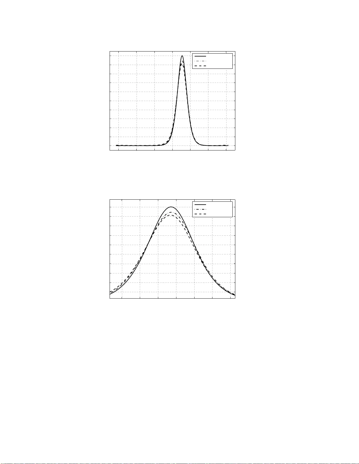
Visco-p oten tial free-surface flo ws and long w a v e mo delling Den y s Dut ykh a , ∗ a CMLA, ENS Cachan, CNRS, PRES UniverSud, 61 Av. Pr esident Wi lson, F-94230 Cachan, F r anc e 1 Abstract In a previous study [DD07b] w e presen ted a no v el visco-p otentia l free surface flo ws form ulation. The go ve rning equations con tain lo cal and nonlo cal dissipativ e terms . F rom ph ysical point of view, lo cal dissipation terms come fr om molecular viscos- it y but i n pract ical co mputations, rather eddy viscosit y should b e used. On the other hand, nonlo cal d issipativ e term repr esen ts a correction due to the p resence of a b ott om b oundary la y er. Using the standard p r o cedure of Boussinesq equations deriv ation, w e co me to nonlo cal long w av e equations. In this article w e analyse disp ersion relation p rop erties of prop osed mo d els. The effect of nonlo cal term on solitary and linear p r ogressiv e wa v es atte n uation is inv estigated. Finally , w e p resen t some computations with viscous Boussinesq equations solv ed by a F ourier typ e sp ectral metho d. Key wor ds: free-surface flo ws , viscous damping, long wa ve mo dels, Boussinesq equations, dissipativ e Kortew eg-de V ries equation, b ottom b ou n dary la y er P ACS: 47.35.Bb, 47.35.Fg , 47.10.ad 1 In tro duction Ev en though the irrotational theory of free-surface flows can predict succe ss- fully man y observ ed wa v e phenomena, viscous effects cannot b e neglected under certain circum stances. Ind eed the que stion of dissipation in p oten tial flo ws of fluid with a free surface is an imp ortant one. As stated b y [ LH92 ], ∗ Corresp ond ing author. Email addr ess: D enys.Duty kh@univ- savoie.fr (Den ys Dut ykh). 1 No w at LAMA, Univ er s it y of Sav oie, CNRS, Campus S cien tifique, 73376 Le Bourget-du-Lac Cedex, F rance Preprint sub mitted to Eu r. J. Mech. B/Fluids Octob er 22, 2018 it w ould b e con v enien t to hav e equations and b oundary conditions of com- parable simplicit y as for undamp ed free-surface flows. The p eculiarity here lies in the fact that the viscous term in the Navie r–Stok es (NS) equations is iden tically equal to zero for a v elo cit y deriving from a p o ten t ia l. There is also a problem with b oundary conditions. It is we ll kno wn that t he usual non-slip condition on the solid b oundaries do es not allow to simulate free surface flo ws in a finite con t ainer. Hence, some further mo difications are required to p ermit the free surface particles to slide along the solid b oundary . These difficulties w ere o v ercome in our recen t w ork [ DD07b ] a nd [ D DZ08 ]. The effects of viscosit y on gravit y wa v es ha v e b een addressed since the end of the nineteen th cen tury in the contex t of the linearized Nav ier–Stok es (NS) equations. It is we ll-kno wn that La m b [ Lam32 ] studied this question in the case of oscillatory w av es on deep water. What is less kno wn is tha t Boussinesq studied this effect as w ell [ Bou95 ]. In this particular case they b oth sho w ed that dα dt = − 2 ν k 2 α, (1) where α denotes the wa v e amplitude, ν t he kinematic viscosit y of the fluid and k = 2 π / ℓ the w av en um b er of the deca ying w av e. Here ℓ stands for the w av elength. This equation leads to the classical law for viscous deca y , namely α ( t ) = α 0 e − 2 ν k 2 t . (2) Let us consider a simple n umerical application with g = 9 . 8 m/s 2 , ℓ = 3 m and molecular viscosit y ν = 10 − 6 m 2 /s . According to the formula ( 2 ), this w av e will tak e t 0 ≈ 8 × 10 4 s or ab out one da y b efore losing one half of its amplitude. This w av e will attain v elo cit y c p = r g k ≈ 2 . 16 m/s and tra v el the distance equal to L = c p · t 0 ≈ 170 k m . This estimation is exaggerated since the classical r esult of Boussinesq a nd Lamb do es not tak e in to account energy dissipation in the b ottom b oundary lay er. W e will discuss the question of linear progressiv e w av es atten uation in Section 5 . Another p oin t is that the molecular viscosit y ν should b e replaced b y eddy viscosit y ν t whic h is more a ppro priate in most practical situations (see Remark 6 fo r more details). The imp ortance of viscous effects f or w ater w av es has b een observ ed in v arious exp erimental studies. F or example, in [ ZG71 ] one can read . . . Ho w ev er, the amplitude disagrees somewhat, and w e supp ose that this migh t b e due to the viscous dissipation. . . [ W u81 ] also mentions this drawbac k of the classical w ater wa v e theory: 2 . . . the p eak a mplitudes observ ed in the exp erimen ts are slightly smaller than those predicted b y the theory . This discrepancy can b e ascrib ed to the neglect of the viscous effects in the theory. . . Another example is the conclusion of [ BPS81 ]: . . . it was found that the inclusion of a dissipativ e term w a s m uc h more im- p ortant than the inclusion of the nonlinear term, although the inclusion of the nonlinear term w as undoubtedly b eneficial in describing the observ a- tions. . . Another source of dissipation is due to b ottom f r iction. An accurate computa- tion of the b ottom shear stress ~ τ is crucial for calculating sedimen t transp o rt fluxes. Consequen tly , the predicted morpholog ical changes will greatly dep end on t he c hosen shear stress mo del. T raditionally , this quantit y is mo delled b y a Ch´ ezy -t yp e la w ~ τ | z = − h = C f ρ | ~ u h | ~ u h , where ~ u h = ~ u ( x, y , − h, t ) is the fluid v elo cit y a t the b o ttom, C f is the friction co efficien t and ρ is the fluid densit y . Two other oft en used laws can b e fo und in [ DD07a , Section 4.3], for example. One problem with this mo del is that ~ τ and ~ u h are in phase. It is well kno wn [ LSV O06 ] that in the case of a laminar b oundary lay er, the b ottom stress ~ τ | z = − h is π 4 out of phase with resp ect to the b ottom v elo cit y . W ater w a v e energy can b e dissipated by differen t ph ysical mec hanisms. The researc h comm unit y agrees at least on one p oin t: the molecular viscosit y is unimp ortant. No w let us discuss more debatable statements . F or example if w e tak e a tsunami wa v e a nd estimate its Reynolds n um b er, w e find Re ≈ 10 6 . So, the flow is clearly t urbulent and in practice it can b e mo delled by v arious eddy viscosit y mo dels . On the other hand, in lab oratory experimen ts the Reynolds n um b er is muc h more mo derat e and sometimes w e can neglect this effect. When non breaking w av es feel the b ottom, the most efficien t mec hanism of energy dissipation is the bo t t o m boundary lay er. This is the fo cus of our pap er. W e briefly discuss the fr ee surface b oundary lay er a nd explain wh y we do not tak e it in to accoun t in this study . Finally , the most imp ortan t (and the most c ha llenging) mec hanism of energy dissipation is wa v e breaking. This pro cess is extremely difficult from the mathematical but also the phy sical and numeric al p oin ts of view since w e ha v e to deal with multiv alued functions, t op ological c ha ng es in the flow and complex turbulen t mixing pro cesses. Now aday s the practitioners can only b e happy to mo del roughly this pro ces s b y a dding ad- ho c dissipativ e terms when the w a v e b ecome s steep enough. In this w ork we k eep the features of undamp ed free-surface flo ws while adding dissipativ e effects. The class ical theory of visc ous p otential flows is based on pressure and b oundary conditions corrections [ JW04 ] due to the presence of 3 viscous stresses. W e presen t here another approa c h. Curren tly , po ten tia l flo ws with ad-ho c dissipativ e terms are used for example in direct n umerical sim ulations of w eak turbulence of gra vit y w av es [ DKZ03 , DKZ04 , ZKPD05 ]. There ha v e also b een sev eral attempts to in tro duce dis- sipativ e effects in to long w av e mo delling [ Mei94 , DD07a , CG07 , Kha97 ]. W e w o uld like to underline that the last pap er [ Kha97 ] contains also a nonlo cal dissipativ e term in time. The presen t w o rk is a direct con tin uation of the recen t studies [ DDZ08 , DD07b ]. In [ DDZ08 ] the authors considered p erio dic w av es in infinite depth a nd deriv a- tion was done in tw o-dimensional (2D) case, while in [ DD0 7 b ] w e remov ed these t w o hypotheses and all the computations are done in 3 D. This po int is imp ortant since the v orticit y structure is more complicated in 3D. In other w o r ds w e considered a g eneral wa v etrain on the free surface of a fluid la y er of finite depth. As a result w e obta ined a formulation whic h contains a nonlo cal term in the b ottom kinematic condition. Later w e discov ered that the nonlo cal term in exactly the same form was deriv ed in [ LO04 ]. The inclusion o f this term is natural since it represen ts the correction to po ten t ia l flow due to the presence of a b oundary la y er. Moreov er, this term is predominan t since its magnitude scales with O ( √ ν ), while o t her terms in the f r ee-surface b oundary conditions a re of order O ( ν ). The imp ortance of this effect w as po in ted out in the classical literat ur e on the sub ject [ Lig78 ]: . . . Bottom friction is the most imp ortant wherev er the w a ter depth is sub- stan tially less than a wa v elength so that the w a v es induce significant hor- izon tal motions near the b o ttom; the asso ciated energy dissipation ta kes place in a b oundary lay er b etw een them and the solid b otto m. . . This quotation means that this type of phenomenon is particularly imp ortant for shallo w w ater wa v es lik e tsunamis, for example [ DD06 , Dut07 ]. Here w e presen t sev eral n umerical computations based on the newly derived gov erning equations and analyse disp ersion r elatio n prop erties. W e w ould lik e to men t ion here a pap er of N. Sugimoto [ Sug91 ]. The author considered initial- v alue problems for the Burgers equation with the inclusion of a hereditary in tegral known as the fractional deriv ative of order 1 2 . The form of this term w as justified in previous w orks [ Sug89 , Sug90 ]. Note, that from fractional calculus p oint of view our nonlo cal term ( 6 ) is also a half-order in tegral. Other researc hers hav e obtained nonlo cal corrections but they differ from ours [ KM75 ]. This discrepancy can b e explained b y a differen t scaling c hosen b y Kakutani & Matsuuc hi in the b oundary la y er. Consequen tly , their go v erning equations contain a nonlo cal term in space. The p erformance of the presen t nonlo cal term ( 6 ) w as studied in [ LSV O06 ]. The authors carr ied out in a wa v e 4 tank a set of exp erimen ts, analyzing the damping and shoaling of solitary w av es. It is shown that the viscous damping due to the b ottom b o undary la y er is w ell represen ted by the no nlo cal term. Their n umerical results fit w ell with the experiments . The mo del not only prop erly predicts the w av e heigh t at a giv en p oint but also pro vides a go o d represen tation o f the c hang es on the shap e and celerit y of the soliton. W e can conclude that the exp erimen tal study b y P . Liu et al. [ LSV O06 ] v alidates t his theory . The presen t article is organized as follo ws. In Section 2 we estimate the rate of viscous dissip ation in differen t regions of the fluid domain. Then, w e presen t basic ideas of deriv ation and come up with visco-p otential free-surface flows form ulation. A t the end of Section 3 we give corresp onding long w av e mo dels : nonlo cal Boussinesq and KdV equations. Section 4 is completely dev ot ed t o the analysis of linear disp ersion relation of complete and long w a v e mo dels in tro duced in previous section. Last tw o sections deal with linear progressiv e and solitary w av es attenuation resp ectiv ely . Finally , the pap er is ended by some conclusions a nd p ersp ectiv es. 2 Anatom y of dissipation In this section w e briefly discuss the con tribution of differen t flo w regions in to w a t er w av e energy dissipation. W e con ven tionally [ Mei94 ] divide t he flow into three regions illustrated o n Figure 1 . On this figure S f and S b stand for free surface and b ottom resp ectiv ely . Then, R i , R f and R b denote the interior region, free surfa ce and b ott om b o undar y lay ers. P S f r a g r e p la c e m e n t s O ~ x z S f S b R f R b R i Figure 1. Conv en tional p artition of the fl o w region in to int erior region and free surface, b ottom b oundary la yers. In order to make some estimates we in tro duce the notation which will b e used in this section: µ is the dynamic viscos it y , δ = O ( √ µ ) is the b oundary la y er 5 thic kness, t 0 is t he c haracteristic time, a 0 is t he c haracteristic w av e a mplitude and ℓ is the w av elength. W e assume tha t the flo w is go v erned by the incompressible Navie r-Stok es equations: ∇ · ~ u = 0 , ∂ ~ u ∂ t + ~ u · ∇ ~ u + 1 ρ ∇ p = ~ g + 1 ρ ∇ · τ , where τ is the viscous stress tensor τ ij = 2 µε ij , ε ij = 1 2 ∂ u i ∂ x j + ∂ u j ∂ x i . W e m ultiply the second equation b y ~ u and in tegrate o ver the doma in Ω with b oundary ∂ Ω to get the follow ing energy bala nce equation: 1 2 Z Ω ∂ ∂ t ρ | ~ u | 2 d Ω + 1 2 Z ∂ Ω ρ | ~ u | 2 ~ u · ~ n dσ = = Z ∂ Ω − p I + τ ~ n · ~ u dσ + Z Ω ρ ~ g · ~ u d Ω − 1 2 µ Z Ω τ : τ d Ω | {z } T . In this identit y eac h term has a precise ph ysical meaning. The left-hand side is the tota l rate of energy c hange in Ω. The second term is the flux o f energy across the b oundary . On the righ t- ha nd side, the first in tegral represen ts the rate o f work by surface stresses acting o n the b oundary . The second integral is the rate of w ork done b y the gravit y force throughout the volume , and the third in tegra l T is the rate of viscous dissipation. W e fo cus o ur atten tion on the last term T . W e estimate the order of magnitude of the rate of dissipation in v arious r egio ns of the fluid. W e start b y the inte rior region R i . Outside the b oundary la y ers, it is reasonable to expect that the rate of strain is dominated by the irrotational part of the v elo cit y whose scale is a 0 t 0 and the length scale is the wa v elength ℓ . The energy dissipation rate is then O T R i ∼ 1 µ µ a t 0 ℓ 2 · ℓ 3 = µ a t 0 2 ℓ ∼ O ( µ ) . Inside the b otto m b oundary la y er the normal gradien t of the solenoidal part 6 of ~ u dominates the strain rate, so tha t O T R b ∼ 1 µ µ a t 0 δ 2 · δ ℓ 2 = µ δ aℓ t 0 2 ∼ O ( µ 1 2 ) . A free surface b oundary lay er also exists . Its impor tance dep ends on the free surface conditions. Consider first the classical case of a clean surface. The stress is mainly controlled by the p otential v elo cit y field whic h is o f the same order as in the main b ody of the fluid. Because of the small v olume O ( δ ℓ 2 ) the r a te o f dissipation in the free surfa ce boundar y lay er is only O T R f ∼ 1 µ µ a t 0 ℓ 2 · δ ℓ 2 = µδ a t 0 2 ∼ O ( µ 3 2 ) . F rom the ph ysical p oin t of view it is we ak er, since only the zero shear stress condition on the f r ee surface is required. Another extreme case is when the free surface is heavily con taminated, for example, b y oil slic ks. The stress in the free surface b o undary la y er can then b e as great as in the b oundary la y er near a solid w all. In the presen t study we do not t r eat suc h extreme situations and the surface con tamination is assumed to b e absen t . The previous scalings suggest the following diagram whic h represen ts the hi- erarc h y o f dissipativ e terms: O µ 1 2 | {z } R b ֒ → O ( µ ) | {z } R i ֒ → O µ 3 2 | {z } R f ֒ → . . . It is clear that the largest energy dissipation tak es place inside the b ottom b oundary la y er. W e take in to a ccoun t only tw o first phenomena fro m this diagram. Consequen tly , all dissipative terms of order O ( µ 3 2 ) and higher will b e neglected. Remark 1 In lab or atory exp e rim ents, surfac e waves ar e c onfine d b y side wal ls as wel l. Th e r ate o f attenuation due to the side-w a l l b oundary layers was c om- pute d in [ ML73 ]. F or sim p l i c ity, in the pr esent study we c onsider an unb ounde d in horizontal c o or din ates domain (s e e Figur e 1 ). 7 3 Deriv ation Consider the linearized 3D incompressible NS equations describing free-surface flo ws in a fluid la y er of unifo rm depth h : ∂~ v ∂ t = − 1 ρ ∇ p + ν ∆ ~ v + ~ g , ∇ · ~ v = 0 , (3) with ~ v the v elo cit y v ector, p the pressure, ρ the fluid densit y and ~ g the acceler- ation due to grav it y . W e represen t ~ v = ( u, v , w ) in the f o rm of the Helmholtz– Lera y decomp osition: ~ v = ∇ φ + ∇ × ~ ψ , ~ ψ = ( ψ 1 , ψ 2 , ψ 3 ) . (4) After substitution of the decomp osition ( 4 ) in to ( 3 ), one notices that the equations a re v erified provided that the functions φ and ~ ψ satisfy the follow ing equations: ∆ φ = 0 , φ t + p − p 0 ρ + g z = 0 , ∂ ~ ψ ∂ t = ν ∆ ~ ψ . Next w e discuss the b oundary conditions. W e assume that the velocity field satisfies t he con v en tional no-slip condition at the b ottom ~ v | z = − h = ~ 0, while at the free surface w e ha v e the usual kinematic condition, which can b e stated as η t + ~ v · ∇ η = w . After linearization it b ecomes simply η t = w . Dynamic condition states that the forces mus t b e equal on b oth sides of t he free surface: [ ~ σ · ~ n ] ≡ − ( p − p 0 ) ~ n + τ · ~ n = 0 at z = η ( x, t ) , where ~ σ is the stress tensor, [ f ] denotes the jump o f a function f a cross the free surface, ~ n is t he normal to the free surface and τ the viscous part of the stress tensor ~ σ . The basic idea consists in expressing the v ortical part o f the v elo cit y field ∇ × ~ ψ in terms of the v elo cit y p oten tial φ and the free surface elev at io n η using differential o r pseudo differen tial op erators. In this section w e just sho w final results while the details of computation can b e fo und in [ DD07b , Dut07 ]. Let us b egin by the free-surface kinematic condition ∂ η ∂ t = w ≡ ∂ φ ∂ z + ∂ ψ 2 ∂ x − ∂ ψ 1 ∂ y , z = 0 . 8 Using the absence of tangen tial stresses o n the free surface, one can replace the r o tational part in the kinematic b oundary condition: η t = φ z + 2 ν ∆ η . In order to accoun t fo r the presence of viscous stresses, we hav e to mo dify the dynamic free-surface condition as we ll. This is done using the balance of normal stresses at the free surface: σ z z = 0 at z = 0 ⇒ p − p 0 = 2 ρν ∂ w ∂ z ≡ 2 ρν ∂ 2 φ ∂ z 2 + ∂ 2 ψ 2 ∂ x∂ z − ∂ 2 ψ 1 ∂ y ∂ z . In [ DD0 7b ] it is sho wn t ha t ∂ 2 ψ 2 ∂ x∂ z − ∂ 2 ψ 1 ∂ y ∂ z = O ( ν 1 2 ), so Bernoulli’s equation b ecomes φ t + g η + 2 ν φ z z + O ( ν 3 2 ) = 0 . (5) Since w e only consider w eak dissipation ( ν ∼ 10 − 6 − 10 − 3 m 2 /s), w e neglect terms of o r der o ( ν ). The second step in our deriv ation consists in introducing a b oundary lay er correction at the b ottom. In the presen t study w e assume the b oundary lay er to b e laminar. The ques tion of turbulen t b oundary lay er w as in ves tigated in [ Liu06 ]. Hence, the b ottom b oundary condition b ecomes ∂ φ ∂ z z = − h = r ν π t Z 0 ∇ 2 ~ x φ 0 | z = − h √ t − τ dτ = − r ν π t Z 0 φ 0 z z | z = − h √ t − τ dτ . (6) One recognizes on the righ t-hand side a half-order integral op erator. The last equation sho ws tha t the effect o f the diffusion pro ce ss in the b oundary la y er is not instan t a neous. The result is cumulativ e and it is w eigh ted b y ( t − τ ) − 1 2 in fa v our of the presen t time. Summarizing the deve lopmen ts made ab ov e and generalizing our equations b y including nonlinear terms, we obtain a set of viscous p oten tial fr ee-surface flo w equations: ∆ φ = 0 , ( ~ x, z ) ∈ Ω = R 2 × [ − h, η ] (7) η t + ∇ η · ∇ φ = φ z + 2 ν ∆ η , z = η (8) φ t + 1 2 |∇ φ | 2 + g η = − 2 ν φ z z , z = η (9) φ z = − r ν π t Z 0 φ z z √ t − τ dτ , z = − h. (10) A t the presen t stage, the addition of nonlinear terms is rather a conjecture. Ho w ev er, a recen t study by Liu et al. [ LPC07 ] suggests that t his conjecture 9 is rather true. The autho rs inv estigated the imp ort ance of nonlinearit y in the b ottom b oundary lay er for a solitary wa v e solution. They came to the conclusion that “t he nonlinear effects are not v ery significant”. Using this we akly da mp ed p oten tial flow f orm ulation and describ ed in previous w o r ks pro cedure [ DD07a , Section 4] of Boussinesq equations deriv ation, one can derive the follow ing system o f equations with horizontal ve lo city ~ u θ defined at the depth z θ = − θh , 0 ≤ θ ≤ 1 : η t + ∇ · (( h + η ) ~ u θ ) + h 3 θ 2 2 − θ + 1 3 ! ∇ 2 ( ∇ · ~ u θ ) = 2 ν ∆ η + r ν π t Z 0 ∇ · ~ u θ √ t − τ dτ , (11) ~ u θ t + 1 2 ∇| ~ u θ | 2 + g ∇ η − h 2 θ 1 − θ 2 ! ∇ ( ∇ · ~ u θ t ) = 2 ν ∆ ~ u θ . (12) F or simplicit y , in this study w e presen t go v erning equations only on the flat b ottom, but generalization can b e done for g eneral bathyme try . Khabakhpa- shev [ Kha87 ], Liu & Or fila [ LO0 4 ] also derive d a similar set of Boussinesq equations in terms of depth-av eraged ve lo city . Our equations ( 11 ) – ( 12 ) ha ve lo cal dissipativ e terms in addition and they are form ula ted in terms o f the v e- lo cit y v ariable defined at arbitrary water lev el that is b eneficial fo r dispersion relation prop erties. 3.1 T otal ene r gy de c ay in visc o-p otential flow Let us consider a fluid lay er infinite in horizon tal co ordinates ~ x = ( x, y ), b ounded b elo w b y the flat b otto m z = − h and a b o v e by the free surface. T otal energy o f w ater w av es is giv en b y the follo wing form ula: E = Z Z R 2 η Z − h 1 2 |∇ φ | 2 dz d~ x + g 2 Z Z R 2 η 2 d~ x. W e would lik e to men tion here that Zakharov sho wed [ Zak68 ] this expression to b e the Hamiltonian for classical w ater w a v e problem with suitable c hoice of canonical v aria bles: η and ψ := φ ( ~ x, z = η , t ). In this section w e are interes ted in t he evolution of the total energy E with time. This question is in v estigated b y computing the deriv ativ e d E dt with resp ect to time t . Obviously , when one considers the classical p oten tial free surface flo w form ulatio n [ Lam32 ], we ha v e d E dt ≡ 0, since no dissipation is in tro duced in to the gov erning equations. W e p erfo rmed the computation of d E dt in t he framew o rk of the visco-p o t en tia l fo rm ulation and giv e here the final result: 10 d E dt = r ν π Z Z R 2 φ t | z = − h t Z 0 φ z z | z = − h √ t − τ dτ d~ x + 2 ν Z Z R 2 ∂ t ( ∇ φ | z = η · ∇ η ) d~ x. In this iden tity , the first term on the right hand side comes from the b oundary la y er and is predominan t in the energy decay since its magnitude scales with O ( √ ν ). The second term has its origins in free surface b oundary conditions. Its magnit ude is O ( ν ), th us it has less imp ort a n t impact on the energy balance. This topic will b e inv estigated further in future studies. 3.2 Dissip ative KdV e quation In this section w e deriv e a viscous Kortew eg-de V ries (KdV) equation f rom just obtained Boussinesq equations ( 11 ), ( 12 ). Since KdV-ty p e equations mo del only unidirectional w av e propagat io n, our a t ten tio n is na turally restricted to 1D case. In order to p erform asymptotic computatio ns, all the equations ha ve to b e switc hed to nondimens ional v aria bles as it is explained in [ DD07a , Sec- tion 2]. W e find the v elo cit y v ariable u in this form: u θ = η + εP + µ 2 Q + . . . where ε , µ are nonlinearit y and disp ersion par a meters respectiv ely (see [ DD07a ] for their definition), P and Q are unkno wn at the presen t momen t. Using the metho ds similar to those used in [ DD07a , Section 6.1], one can easily sho w that P = − 1 4 η 2 , Q = θ − 1 6 − θ 2 2 η xx . This result immediately yields the follow ing asymptotic represen tation of the v elo cit y field u θ = η − 1 4 εη 2 + µ 2 θ − 1 6 − θ 2 2 η xx + . . . (13) Substituting the last formula ( 13 ) in to equation ( 1 1 ) and switc hing again to dimensional v ariables, o ne o bta ins this visc ous KdV-type equation: η t + r g h ( h + 3 2 η ) η x + 1 6 h 3 η xxx − r ν π t Z 0 η x √ t − τ dτ = 2 ν η xx . (14) This equation will b e used in Section 5 t o study the damping of linear progres- siv e w av es. Inte gral damping terms are reasonably w ell kno wn in the con text of KdV type equations. V arious nonlo cal corrections can b e found, for example, in the fo llo wing references [ BS71 , Che68 , Mil76 , GPT03 ]. A similar no nlo cal K dV equation w as already deriv ed in [ KM75 ]. They used a differen t scaling in b oundary lay er whic h resulted in dissipativ e term nonlo- 11 cal in space. Later, Matsuuc hi [ Mat76 ] p erformed a comparison of n umerical computations with their mo del equation a gainst lab oratory data. They show ed that their mo del do es not repro duce w ell the phase shift: . . . it may b e concluded tha t our mo dified K-dV equation can desc rib e the observ ed w a v e b eha viours except the fact that the phase shift obtained b y the calculatio ns is not confirmed by their exp eriments . Excellen t p erformance of the mo del ( 14 ) with resp ect to exp erimen ts was sho wn in [ LSVO06 ]. 4 Disp ersion relation of complete and Boussinesq nonlo cal equa- tions In t eresting information ab o ut the gov erning equations can b e obtained fro m the linear disp ersion relation analysis. In t his section we are going to analyse the new set of equations ( 7 )–( 10 ) f or the complete w ater wa v e pro blem and the corr espo nding long w av e asymptotic limit ( 11 ) , ( 12 ). T o simplify the computatio ns, w e consider the tw o-dimensional problem. The generalization to higher dimensions is straigh tforw ard and is p erfor med b y replacing the w av en umber k b y its mo dulus | ~ k | in v ectorial case. T raditionally the gov erning equations are linearized and the b otto m is assumed t o b e flat. The last h yp o thesis is made thr o ughout this study . After all these simplifica- tions the new set of equations b ecomes φ xx + φ z z = 0 , ( x, z ) ∈ R × [ − h, 0] , (15) η t = φ z + 2 ν η xx , z = 0 , (16) φ t + g η + 2 ν φ z z = 0 , z = 0 , (17) φ z + r ν π t Z 0 φ z z √ t − τ dτ = 0 , z = − h. (18) The next classical step consists in finding solutions of the sp ecial for m φ ( x, z , t ) = ϕ ( z ) e i ( kx − ω t ) , η ( x, t ) = η 0 e i ( kx − ω t ) . (19) F rom con tin uity equation ( 15 ) w e can determine the structure of the function ϕ ( z ): ϕ ( z ) = C 1 e k z + C 2 e − k z . Altogether w e hav e three unknown constan ts 2 ~ C = ( C 1 , C 2 , η 0 ) and three b oundary conditio ns ( 16 )–( 18 ) whic h can b e view ed as a linear system with 2 Since the presen t problem is linear, w e ha ve effectiv ely only t wo degrees of freedom 12 resp ect to ~ C : M ~ C = ~ 0 . (20) The matrix M has the follo wing elemen ts M = k − k iω − 2 ν k 2 iω − 2 ν k 2 iω − 2 ν k 2 − g e − k h 1 + k F ( t, ω ) e k h − 1 + k F ( t, ω ) 0 where the function F ( t, ω ) is defined in the following w a y: F ( t, ω ) := r ν π t Z 0 e iω ( τ )( t − τ ) √ t − τ dτ . (21) In order to hav e non trivial solutions of ( 15 )–( 18 ), the determinan t o f the sys- tem ( 20 ) has to b e equal to zero det M = 0. It give s us a relatio n b etw een ω and w av en um b er k . This relation is called the linear disp ersion relation: D ( ω , k ) := ( iω − 2 ν k 2 ) 2 + g k ta nh( k h ) − k F ( t, ω ) ( iω − 2 ν k 2 ) 2 tanh( k h ) + g k ≡ 0 . (22) A similar pro cedure can b e follo w ed for Boussinesq equations ( 11 ), ( 12 ). W e do not give here the details o f the computations but only the final result: D b ( ω , k ) := ( iω − 2 ν k 2 ) 2 + b ( k h ) 2 iω ( iω − 2 ν k 2 ) + g hk 2 (1 − a ( k h ) 2 ) − g k 2 F ( t, ω ) ≡ 0 , (23) where w e introduced the following notation: a := θ 2 2 − θ + 1 3 , b := θ 1 − θ 2 . Unfortunately , the r elat io ns D ( ω , k ) ≡ 0 and D b ( ω , k ) ≡ 0 cannot b e solved analytically to giv e an explicit dep endence of ω on k as for the classic al wa- ter w av e problem. Consequen t ly , w e apply a quadrature fo rm ula to discretize the nonlo cal term F ( t n , ω ), where t n denotes the discrete time v a riable. The resulting algebraic equation with resp ect to ω ( t n ; k ) is solv ed analytically . Remark 2 Con tr ary to the c l a s sic al water wave pr ob l e m a n d, by c onse quenc e, standar d Boussinesq e quations ( their disp ersion r elation c an b e found in [ DD07a , Se ction 3.2], for example ) wher e the disp ersion r elation do es not dep end on time ω 2 − g k tanh( k h ) ≡ 0 , (24) her e we have a d ditional ly the dep endenc e o f ω ( k ; t ) on time t as a p a r ame- ter. It is a c onse quenc e of the pr esenc e o f the nonl o c al term in time in the but it is not imp ortan t for our pu rp oses. 13 b ottom b oundary c ond i tion ( 10 ). Physic al ly it me an s that the b oundary layer “r ememb ers” the flow history. Remark 3 The r e is one subtle p oint in the deriv ation pr ese n te d ab o v e . In fact, al l c omputations wer e p erforme d as if the fr e quency ω wer e indep endent fr om time. Our final r esult s hows that time t ap p e ars explicitly in the dis - p ersion r elations ( 22 ), ( 23 ) . Developments made ab ove make sense under the assumption of slo w variation of ω with time t . This statement c an b e writ- ten i n mathematic al form ∂ ω ∂ t ≪ 1 . It is r ather a c onje ctur e her e and wil l b e examin e d in futur e studies. We had to make this a s sumption in or der to avoid c omplic ate d inte g r o-differ ential e quations and, c onse quently, simplify the analysis. 4.1 A n alytic al limit for in finite time In the previous section w e sho w ed that the disp ersion relation of our visco- p oten tial formulation is time dep enden t . It is natural to ask what happ ens when time ev olv es. Here w e compute the limiting state of the disp ersion curv es ( 22 ), ( 23 ) as t → + ∞ . Namely , w e will take this limit in equations ( 2 2 ), ( 2 3 ) assuming, of course, tha t it exists ∃ ω ∞ ( k ) := lim t → + ∞ ω t ( k ) . Time t comes in disp ersion relations through the argumen t of the function F ( t, ω ) defined in ( 21 ). Its limit can b e easily computed to giv e lim t → + ∞ F ( t, ω ) = s ν π ω ∞ + ∞ Z 0 e ip √ p dp = s ν ω ∞ e i π 4 . No w we are ready to write down the final results: D ( ω ∞ , k ) := ( iω ∞ − 2 ν k 2 ) 2 + g k ta nh( k h ) − s ν ω ∞ k e i π 4 ( iω ∞ − 2 ν k 2 ) 2 tanh( k h ) + g k ≡ 0 , D b ( ω ∞ , k ) := ( iω ∞ − 2 ν k 2 ) 2 + b ( k h ) 2 iω ∞ ( iω ∞ − 2 ν k 2 ) + g hk 2 (1 − a ( k h ) 2 ) − g k 2 s ν ω ∞ e i π 4 ≡ 0 . 14 In order to solv e nume rically nonlinear equation D ( ω ∞ , k ) = 0 (or D b ( ω ∞ , k ) = 0 when one is in terested in Boussinesq equations) with resp ect to ω ∞ , w e apply a Newton-type metho d. The iterations con v erg e very quic kly since w e use analytical expressions for the Jacobian dD dω ∞ ( dD b dω ∞ , corresp ondingly). Deriv ativ e computation is straightforw ard. Limiting disp ersion curv es are plot t ed (see Figure 7 ) and discussed in the next section. 4.2 Discussion Numerical snapshots of the no nclassical disp ersion relation 3 at differen t times for complete and Boussines q equations are g iv en on Figures ( 2 )–( 6 ). The v alue of the eddy viscosit y ν is tak en from T a ble 1 and w e consider a one meter depth fluid la y er ( h = 1 m). W e will try to make sev eral commen ts on the o btained results. Remark 4 R e c al l that these snapshots wer e obtain e d under the assumption that ω is slow ly varying in time. The validity of this appr oxim a tion is exa m ine d and discusse d in [ Dut08 ]. Just a t the b eginning (when t = 0) , there is no effect of the nonlo cal term. This is why on Figure 2 new and classical 4 curv es are sup erimp osed. With no surprise, the phase v elo cit y of Boussinesq equations represen ts w ell only long w av es limit (let us say up to k h ≈ 2). When time ev olv es, w e can see tha t the main effect of nonlo cal term consists in slow ing down long w av es (see Figures 3 – 5 ). Namely , in the vicinit y of k h = 0 the real part of the phase v elo cit y is sligh tly smaller with r esp ect to the classical formulation. F rom ph ysical p oin t of view this situation is comprehensible since only long w a v es “feel” the b ottom and, by consequence, are affected b y b ottom b o undary la y er. On the other hand, the imaginary part of the phase v elo cit y is resp onsible for the wa v e amplitude attenuation. The minim um of Im c p ( k ) in the region of long w a v es indicates that there is a “preferred” w a v elength whic h is attenu ated the most. In the range of short w a v es the imaginary part is monotonically decreasing. In practice it means that high-f requency comp onents are damp ed b y the mo del. This prop erty can be adv an tageous in n umerics, for example. On Figure 6 w e depicted the real part of c p ( k ) with zo om made on long and mo derate w av es. The reader can see that nonlo cal full and Boussinesq equations ha v e similar b eha viour in the vicinit y of k h = 0. 3 T o b e precise, we plot real and imaginary p arts of the dimensionless p hase v elocity whic h is defined as c p ( k ) := 1 √ g h ω ( k ) k . 4 In this section expression “classical” refers to complete w ater w av e problem or its disp ersion relation corresp ond ingly . 15 0 2 4 6 8 10 12 0.2 0.4 0.6 0.8 1 Re c p /(gh) 1/2 Nonlocal equations Classical equations Nonlocal Boussinesq Classical Boussinesq 0 2 4 6 8 10 12 −0.02 −0.015 −0.01 −0.005 0 kh Im c p /(gh) 1/2 Nonlocal equations Nonlocal Boussinesq Figure 2. Real and im aginary part of disp er s ion cu r v e at t = 0. At the b eg inning, the nonlo cal term has no effect. T h us, the r eal parts of the classical water w a ve pr oblem and new set of equ ations are exactly s up erimp osed on this fi gure. T he imaginary part represen ts only local dissipation at this stage. No w let us discuss the limiting state of phase ve lo city curv es as t → + ∞ . It is depicted on Figure 7 . One can see singular b eha viour in the vicinity of zero. This situation is completely normal since v ery long w av es are highly affected b y b ottom b oundary la y er. W e w ould lik e to commen t more on the b eha viour of curv es o n F igure 7 since it is not easy t o distinguish them with graphical resolution. W e will concen tra t e on the upp er image b ecause ev erything is clear b elo w with imaginary part. In the vicinit y of k h = 0 we ha v e the sup erp osition of nonlo cal models (complete set of equations ( 7 ) – ( 1 0 ) and Boussinesq equations ( 11 ) – ( 12 )). When w e gradually mov e to short w av es, w e hav e t he sup erp osition of complete clas- sical and nonlo cal ( 7 ) – ( 10 ) water wa v e problems. Mean while, Boussinesq system giv es sligh tly differen t phase v elo cit y for k h ≥ 3. This is comprehen- sible since we cannot simplify considerably the problem and ha v e uniformly go o d approx imation ev erywhere. V arious Boussinesq systems ar e designed to repro duce the b eha viour of long wa v es. 5 A tten uation of linear progressiv e wa v es In this Section we in v estigate the damping r a te of linear progressiv e w av es. Th us, the first step consists in linearizing dissipativ e KdV equation ( 14 ) to 16 0 2 4 6 8 10 12 0.2 0.4 0.6 0.8 1 Re c p /(gh) 1/2 0 2 4 6 8 10 12 −0.02 −0.015 −0.01 −0.005 0 kh Im c p /(gh) 1/2 Nonlocal equations Classical equations Nonlocal Boussinesq Classical Boussinesq Nonlocal equations Nonlocal Boussinesq Figure 3. Ph ase velocit y at t = 1. Boundary la yer effects start to b e visible: the real part of the v elo cit y sligh tly d r ops do wn and the straigh t lines of the imaginary part are deformed by the non lo cal term. Within graph ical accuracy , the classical and their nonlo cal coun terp arts are sup erimp osed. 0 2 4 6 8 10 12 0.2 0.4 0.6 0.8 1 Re c p /(gh) 1/2 0 2 4 6 8 10 12 −0.02 −0.015 −0.01 −0.005 0 kh Im c p /(gh) 1/2 Nonlocal equations Classical equations Nonlocal Boussinesq Classical Boussinesq Nonlocal equations Nonlocal Boussinesq Figure 4. Ph ase v elocity at t = 2. Nonlo cal term slows do wn long w av es since th e real part of the p hase v elo cit y decreases. obtain the follo wing nonlo cal Airy equation: η t + r g h hη x + 1 6 h 3 η xxx − r ν π t Z 0 η x √ t − τ dτ = 2 ν η xx (25) In other w ords, w e can say that we r estrict our atten tion o nly to small ampli- tude wa v es. No w we mak e the next assumption. W e lo ok for a particular form 17 0 2 4 6 8 10 12 0.2 0.4 0.6 0.8 1 Re c p /(gh) 1/2 0 2 4 6 8 10 12 −0.02 −0.015 −0.01 −0.005 0 kh Im c p /(gh) 1/2 Nonlocal equations Classical equations Nonlocal Boussinesq Classical Boussinesq Nonlocal equations Nonlocal Boussinesq Figure 5. Ph ase v elocit y at t = 4. On Figure 6 w e p lot a zo om on long and mod erate w a ves. 0 0.5 1 1.5 2 0.7 0.75 0.8 0.85 0.9 0.95 1 kh Re c p (k)/(gh) 1/2 Nonlocal equations Classical equations Nonlocal Boussinesq Classical Boussinesq (a) Zo om on long w a ves. Classical and corresp ondin g Boussinesq equations are almost sup erimp osed in this region. 2 2.2 2.4 2.6 2.8 3 0.58 0.6 0.62 0.64 0.66 0.68 0.7 kh Re c p (k)/(gh) 1/2 Nonlocal equations Classical equations Nonlocal Boussinesq Classical Boussinesq (b) Z o om on mo derate wa v elengths. In this region classical and nonlo cal com- plete equations are almost su p erim- p osed. In the same time one can n otice a little difference in Boussinesq mod els. Figure 6. Real part of the phase v elo cit y at t = 4. of the solutions: η ( x, t ) = A ( t ) e ik ξ , ξ = x − q g ht. (26) where k is the w a v enum b er and A ( t ) is called the complex amplitude, since | η ( x, t ) | = |A ( t ) | . In tegr o -differen tial equation gov erning the temp oral ev olu- tion o f A ( t ) can b e easily derived by substituting the sp ecial represen tat io n ( 26 ) into linearized KdV equation ( 25 ): d A dt − i 6 r g h ( k h ) 3 A ( t ) + 2 ν k 2 A ( t ) − ik r g ν π h t Z 0 A ( τ ) √ t − τ dτ = 0 . (27) 18 0 2 4 6 8 10 12 14 0.2 0.4 0.6 0.8 1 kh Re c p (k)/(gh) 1/2 Phase velocity at t = + ∞ Nonlocal equations Classical equations Nonlocal Boussinesq 0 2 4 6 8 10 12 14 −0.1 −0.08 −0.06 −0.04 −0.02 0 kh Im c p (k)/(gh) 1/2 Nonlocal equations Nonlocal Boussinesq Figure 7. Limiting steady state of th e phase v elo cit y at t → + ∞ . In our applications we a r e rather in terested in tempor a l ev olution o f the ab- solute v a lue |A ( t ) | . It is straigh tforw ard to deriv e the gov erning equation for the squared wa v e amplitude: d |A| 2 dt + 4 ν k 2 |A ( t ) | 2 − ik r g ν π h t Z 0 ¯ A ( t ) A ( τ ) − A ( t ) ¯ A ( τ ) √ t − τ dτ = 0 . If we denote b y A r ( t ) and A i ( t ) real and imaginar y parts of A ( t ) resp ectiv ely , the la st equation can b e further simplified: d |A| 2 dt + 4 ν k 2 |A ( t ) | 2 + 2 k r g ν π h t Z 0 A r ( t ) A i ( τ ) − A i ( t ) A r ( τ ) √ t − τ dτ = 0 . (28) Just deriv ed integro-differen tial equation represen ts a generalisation to the classical equation ( 1 ) b y Boussinesq [ Bou95 ] and Lamb [ Lam32 ] for t he peri- o dic, linear w av e amplitude ev olution in a visc ous fluid. W e recall that no v el in tegral term is a direct conseq uence of the b o ttom b oundary la y er mo delling. Unfortunately , equation ( 28 ) cannot b e used directly for numeric al computa- tions since w e need to kno w the follow ing combin ation of real and imaginary parts A r ( t ) A i ( τ ) − A i ( t ) A r ( τ ) for τ ∈ [0 , t ]. It represen t s a new and non- classical asp ect o f the presen t theory . Equation ( 28 ) allo ws us to discuss the relativ e imp ortance of lo cal and nonlo- cal dissipativ e terms for long w av es. In fact, when w e consider the deep-w a t er appro ximation, only lo cal dissipativ e terms are presen t in the go v erning equa- tions [ DDZ08 ]. On the other hand, in shallo w w aters the in tegral term is predominan t . It means that there is an intermed iate depth where bot h dissi- 19 p ar ameter definition value ν eddy viscosit y 10 − 3 m 2 s g gra vity accele ration 9 . 8 m s 2 h w ater depth 3600 m ℓ w a vele ngth 50 k m k w a ven umb er = 2 π ℓ m − 1 T able 1 V alues of the p arameters u sed in the numerical computations of the linear progres- siv e w a ves amplitude. These v alues corresp ond to a t ypical I ndian Ocean tsunami. pativ e terms hav e equal magnitude. This depth can b e estimated when one switc hes to dimensionless fo rm of the equation ( 28 ). Comparing the co effi- cien ts in fron t of dissipativ e terms g iv es the following transcenden tal equation for the “critical” depth h ∗ : h ∗ = g 4 π ω ν k 2 where ω is the c haracteristic w a v e frequency . In n umerical computations it is adv an tageous to in tegrate exactly lo cal terms in equation ( 27 ). It is done b y ma king the following c ha ng e of v ariables: A ( t ) = e − 2 ν k 2 t e i 6 √ g h ( kh ) 3 t ˜ A ( t ) . One can easily show that new function ˜ A ( t ) satisfies the following equation: d ˜ A dt = ik r g ν π h t Z 0 e 2 ν k 2 ( t − τ ) e − i 6 √ g h ( kh ) 3 ( t − τ ) √ t − τ ˜ A ( τ ) dτ On Figure 8 we plot a solution of integro-differen tial equation ( 27 ). All pa- rameters related to this case are giv en in T able 1 . These v alues w ere c hosen to sim ulate a ty pical tsunami in Indian Ocean [ DD06 ]. W e ha ve to say that the w av e amplitude damping is en tirely due to the dissipation in b o undary la y er since lo cal terms ar e unimp o rtan t for sufficien tly long w a ves . It means that classical formula ( 2 ) give s almo st constan t v alue α 0 of the amplitude α ( t ) on the time scale of sev eral hours, since the factor 2 ν k 2 is of o rder ≈ 10 − 11 for parameters giv en in T able 1 . 6 Solitary wa v e propagation In this section w e w ould lik e to sho w the effect of nonlo cal term on the solitary w av e atten uation. F or simplicit y , w e will consider wa v e propagat io n in a 1D 20 0 1 2 3 4 5 6 0.9 0.92 0.94 0.96 0.98 1 1.02 t, hours |A(t)|/|A(0)| Amplitude of linear progressive waves Figure 8. Amplitude of linear p rogressiv e w a ves as a function of time. V alues of all parameters are giv en in T able 1 . c ha nnel. The question of the b ottom shear stress effect on the solitary w av e propagation w a s considered for the first time in [ Keu48 ]. F or n umerical in tegration of equations ( 11 ), ( 12 ) w e use the same F ourier- t yp e sp ectral metho d tha t w a s describ ed in [ DD0 7 a , Section 5]. Obviously this metho d has to b e sligh tly adapted b ecause of the presence of nonlo cal in time term. W e hav e to say that this term neces sitates the storage of ∇ · ~ u ( n ) at previous time steps. Hence, lo ng time computations can b e memory consuming. The v alues of all dimensionle ss pa rameters a re giv en in T able 2 . D imensionless viscosit y ν is related to other physic al parameters in the follo wing w ay: ν 2 = ¯ ν ℓ √ g h , where ¯ ν is kinematic viscosit y , ℓ is the c haracteristic wa v elength and h is the t ypical depth. Remark 5 F r om numeric al p oin t o f view, the inte gr al term t R 0 φ z z ( ~ x, − h,τ ) √ t − τ dτ c an p ose some pr oblem s in the vicinity of the upp er limit τ = t . Pr ob ably the b est way to de al with this pr oblem is to sep ar ate the inte gr al in two p arts: t Z 0 φ z z ( ~ x, − h, τ ) √ t − τ dτ = t − δ Z 0 φ z z ( ~ x, − h, τ ) √ t − τ dτ + t Z t − δ φ z z ( ~ x, − h, τ ) √ t − τ dτ , δ > 0 . The first inte gr al c an b e c ompute d in a usual wa y without any sp e cia l c ar e. Then one a p plies to the se c ond inte gr al a sp e cial clas s of Gauss quadr atur e 21 p ar ameter definition value ε nonlinearit y 0 . 02 µ disp ersion 0 . 06 ν eddy viscosit y 0 . 001 c soliton v elo city 1 . 0 2 θ z θ = − θ h 1 − √ 5 / 5 x 0 soliton cen ter at t = 0 − 1 . 5 T able 2 V alues of the dimensionless parameters used in the n umerical computations. formulas with weighting func tion ( t − τ ) − 1 2 . But ther e is another wel l-known trick that we des crib e her e. This te chnique c an b e i m plemente d in simpler way. We r ewrite our inte gr al in the fo l lowing way t Z 0 φ z z ( ~ x, − h, τ ) √ t − τ dτ = t Z 0 φ z z ( ~ x, − h, t ) √ t − τ dτ + t Z 0 φ z z ( ~ x, − h, τ ) − φ z z ( ~ x, − h, t ) √ t − τ dτ . The fi rs t inte gr al in the right hand si d e c an b e evaluate d analytic al ly whi l e the se c ond on e do e s not c ontain any singularity under the assumption o f differ en- tiability of τ 7→ φ z z ( ~ x, − h, τ ) at τ = t : t Z 0 φ z z ( ~ x, − h, τ ) √ t − τ dτ = 2 √ tφ z z ( ~ x, − h, t ) + t Z 0 φ z z ( ~ x, − h, τ ) − φ z z ( ~ x, − h, t ) √ t − τ dτ . Remark 6 What is the value of ν to b e taken in numeric al simulations? T her e is surprisingly little publishe d information of this s ubje ct. What is cle ar is that the mole cular d iffusion is to o smal l to mo del true visc ous damping and one should r ather c onsider the e ddy visc os ity p ar ameter. Som e inter esting infor- mation on this subje ct c an b e found in [ TSL07 ]: We have sp ent a c onsi d er able amount of time and effort se eking further publishe d i n formation on visc ous effe c ts on ship waves. This se n tenc e c onfirms our appr ehension. The authors of this w o rk c ame to the fo l lowing c onclusion . . . we r eiter ate that a visc osity o f ab out ν = 0 . 00 5 m 2 /s ga ve r e ason- able agr e eme nt w i th longitudinal cut r esults (including app ar ent dam ping of tr ansverse waves). 22 In ano ther famous p ap er [ BPS8 1 ] one c an find: . . . Such a de c ay r a te le a ds to a value for µ in ( M ∗ ) o f 0.014. . . In their work µ is the c o efficie nt in fr ont of the di s s ip ative term i n BB M e quation: η t + η x + 3 2 η η x − µη xx − 1 6 η xxt = 0 . It is i m p ortant to underlin e that this e quation is written in dime n sionless variables. Thus, the value r ep orte d in that study has to b e r esc ale d with r esp e ct to other physic al p ar ameters. Liu and Orfil la [ LO04 ] r ep ort the value of e ddy visc osi ty ν = 0 . 001 m 2 /s . If we summarize al l the r emarks made ab ove, we c an c onclude that the value of the or der 10 − 3 – 10 − 2 m 2 /s should give r e asonable r es ults. 6.1 Appr oximate solitary wave s o lution In order to provide an initial condition for equations ( 11 ), ( 1 2 ), w e are going to o bt a in an approx imate solitary w av e solution for nondissipativ e 1D v ersion of these equations ov er the flat b ottom: η t + (1 + εη ) u x + µ 2 θ 2 2 − θ + 1 3 u xxx = 0 , u t + η x + ε 2 ( u 2 ) x − µ 2 θ 1 − θ 2 u xxt = 0 . Then, w e apply the same approac h as in Section 3.2 or in [ DD 0 7a , Section 6.1]. W e do not pro vide the computatio ns here since they are simple and can b e done without a ny difficulties. The final result is the fo llowing: η ( x, t ) = 2( c − 1) ε sec h 2 q 6( c − 1) 2 µ ( x + x 0 − ct ) and the v elo city is given by f orm ula ( 13 ). In the numerical results presen ted here, we use η ( x, 0 ) and u ( x, 0) as initial conditions. 6.2 Discussion On F igures 9 – 11 w e presen t three curv es. They depict the free surface elev a- tion according to thr ee differen t formulations. The first corresp onds t o classical 23 −3 −2 −1 0 1 2 3 0 0.2 0.4 0.6 0.8 1 1.2 1.4 1.6 1.8 2 t = 0.500 x η No dissipation Local Nonlocal Figure 9. Comparison among t wo d issipativ e and nond issipativ e Boussinesq equa- tions. Snapshots of the f ree surface at t = 0 . 5 −3 −2 −1 0 1 2 3 0 0.2 0.4 0.6 0.8 1 1.2 1.4 1.6 1.8 2 t = 1.000 x η No dissipation Local Nonlocal Figure 10. Comp arison among t wo diss ip ativ e and nondissipativ e Boussinesq equa- tions. Snapshots of the f ree surface at t = 1 . 0 Boussinesq equations without dissipation. The second one to dissipativ e sys- tem with differential or lo cal terms (for example, ν ∆ ~ u in momentum conser- v ation equation) and the third curv e corresponds to the new set of equations ( 11 ), ( 1 2 ). On Fig ure 12 w e made a zo om on the soliton crest. It can b e seen that Boussinesq equations with nonlo cal term provide stronger atten uation of the a mplitude. In the same time, as it was sho wn in the previous section, this nonlo cal term sligh tly slo ws do wn the solitary w a v e. In order to sho w explicitly the rate of amplitude attenu ation, w e plot on Fig- 24 −3 −2 −1 0 1 2 3 0 0.2 0.4 0.6 0.8 1 1.2 1.4 1.6 1.8 2 t = 2.000 x η No dissipation Local Nonlocal Figure 11. Comp arison among t wo diss ip ativ e and nondissipativ e Boussinesq equa- tions. Snapshots of the f ree surface at t = 2 . 0 0 0.2 0.4 0.6 0.8 1 1.2 0.2 0.4 0.6 0.8 1 1.2 1.4 1.6 1.8 2 t = 2.000 x η No dissipation Local Nonlocal Figure 12. Comp arison among t wo diss ip ativ e and nondissipativ e Boussinesq equa- tions. Zo om on the solito n crest at t = 2 . 0 ure 13 t he graph of the following application t → sup − π
Original Paper
Loading high-quality paper...
Comments & Academic Discussion
Loading comments...
Leave a Comment