Learning to Pivot with Adversarial Networks

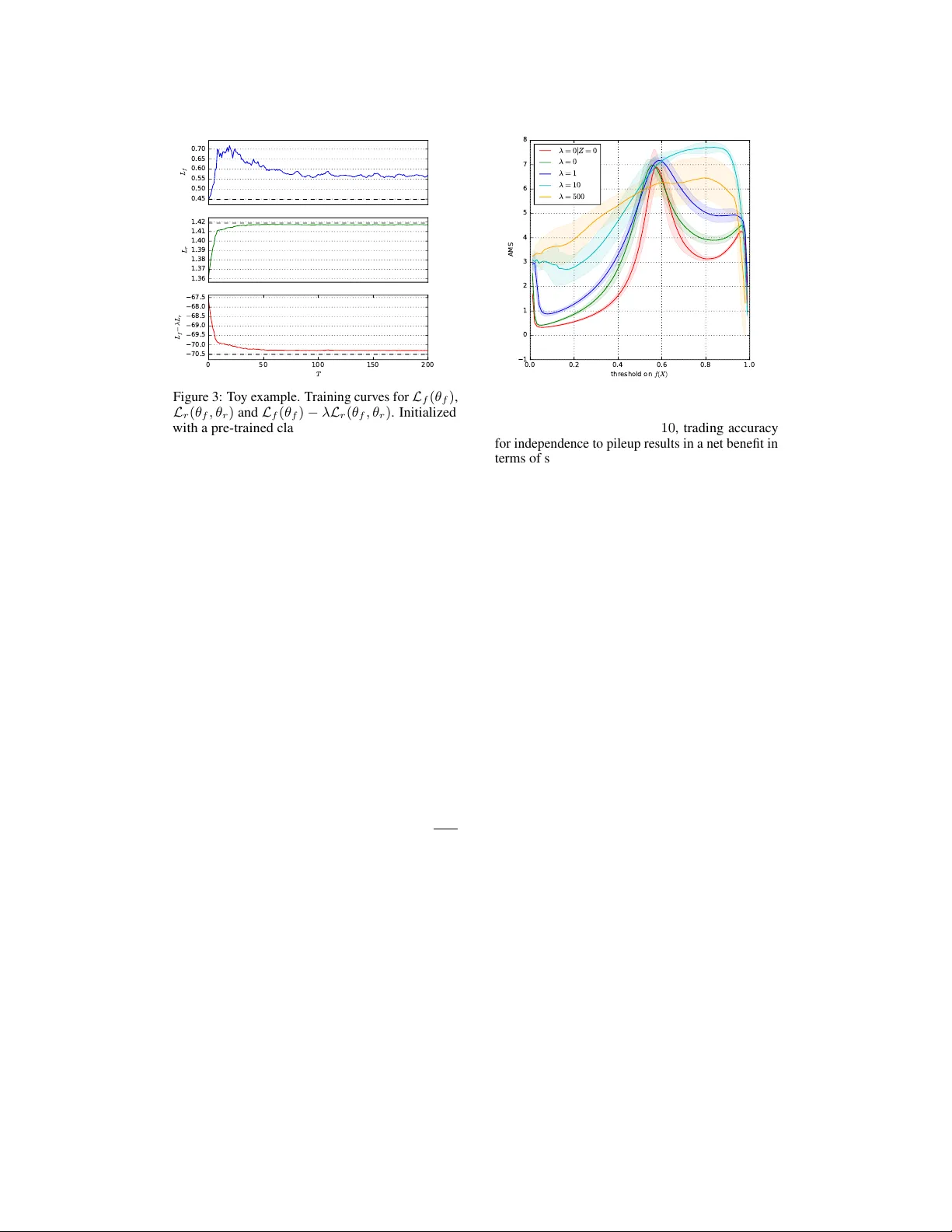
Lear ning to Piv ot with Adv ersarial Networks Gilles Louppe New Y ork Univ ersity g.louppe@nyu.edu Michael Kagan SLA C National Accelerator Laboratory makagan@slac.stanford.edu K yle Cranmer New Y ork Univ ersity kyle.cranmer@nyu.edu Abstract Sev eral techniques for domain adaptation hav e been proposed to account for dif ferences in the distrib ution of the data used for training and testing. The majority of this w ork focuses on a binary domain label. Similar problems occur in a scientific context where there may be a continuous family of plausible data generation processes associated to the presence of systematic uncertainties. Robust inference is possible if it is based on a piv ot – a quantity whose distribution does not depend on the unknown v alues of the nuisance parameters that parametrize this family of data generation processes. In this work, we introduce and deriv e theoretical results for a training procedure based on adversarial networks for enforcing the piv otal property (or , equiv alently , fairness with respect to continuous attributes) on a predicti ve model. The method includes a hyperparameter to control the trade- off between accuracy and robustness. W e demonstrate the ef fectiv eness of this approach with a toy example and e xamples from particle physics. 1 Introduction Machine learning techniques hav e been used to enhance a number of scientific disciplines, and they hav e the potential to transform ev en more of the scientific process. One of the challenges of applying machine learning to scientific problems is the need to incorporate systematic uncertainties, which affect both the rob ustness of inference and the metrics used to ev aluate a particular analysis strategy . In this work, we focus on supervised learning techniques where systematic uncertainties can be associated to a data generation process that is not uniquely specified. In other words, the lack of systematic uncertainties corresponds to the (rare) case that the process that generates training data is unique, fully specified, and an accurate representativ e of the real world data. By contrast, a common situation when systematic uncertainty is present is when the training data are not representative of the real data. Sev eral techniques for domain adaptation ha ve been developed to create models that are more robust to this binary type of uncertainty . A more generic situation is that there are se veral plausible data generation processes, specified as a family parametrized by continuous nuisance parameters, as is typically found in scientific domains. In this broader conte xt, statisticians have for long been working on robust inference techniques based on the concept of a pi vot – a quantity whose distribution is in v ariant with the nuisance parameters (see e.g., (Degroot and Schervish, 1975)). Assuming a probability model p ( X, Y , Z ) , where X are the data, Y are the target labels, and Z are the nuisance parameters, we consider the problem of learning a predicti ve model f ( X ) for Y conditional on the observed v alues of X that is robust to uncertainty in the unkno wn value of Z . W e introduce a flexible learning procedure based on adversarial netw orks (Goodfello w et al., 2014) for enforcing that f ( X ) is a piv ot with respect to Z . W e deri ve theoretical results proving that the procedure con verges tow ards a model that is both optimal and statistically independent of the nuisance parameters (if that model exists) or for which one can tune a trade-of f between accurac y and robustness (e.g., as dri ven by a higher le vel objectiv e). In particular, and to the best of our knowledge, our contrib ution is the first solution for imposing pi votal constraints on a predicti ve model, w orking regardless of the 31st Conference on Neural Information Processing Systems (NIPS 2017), Long Beach, CA, USA. Classifier f X θ f f ( X ; θ f ) L f ( θ f ) ... Adversary r γ 1 ( f ( X ; θ f ); θ r ) γ 2 ( f ( X ; θ f ); θ r ) . . . θ r ... Z p θ r ( Z | f ( X ; θ f )) P ( γ 1 , γ 2 , . . . ) L r ( θ f , θ r ) Figure 1: Architecture for the adversarial training of a binary classifier f against a nuisance parameters Z . The adversary r models the distribution p ( z | f ( X ; θ f ) = s ) of the nuisance parameters as observed only through the output f ( X ; θ f ) of the classifier . By maximizing the antagonistic objective L r ( θ f , θ r ) , the classifier f forces p ( z | f ( X ; θ f ) = s ) tow ards the prior p ( z ) , which happens when f ( X ; θ f ) is independent of the nuisance parameter Z and therefore pi votal. type of the nuisance parameter (discrete or continuous) or of its prior . Finally , we demonstrate the effecti veness of the approach with a toy e xample and examples from particle physics. 2 Problem statement W e be gin with a family of data generation processes p ( X, Y , Z ) , where X ∈ X are the data, Y ∈ Y are the tar get labels, and Z ∈ Z are the nuisance parameters that can be continuous or cate gorical. Let us assume that prior to incorporating the ef fect of uncertainty in Z , our goal is to learn a regression function f : X → S with parameters θ f (e.g., a neural network-based probabilistic classifier) that minimizes a loss L f ( θ f ) (e.g., the cross-entropy). In classification, values s ∈ S = R |Y | correspond to the classifier scores used for mapping hard predictions y ∈ Y , while S = Y for regression. W e augment our initial objectiv e so that inference based on f ( X ; θ f ) will be robust to the value z ∈ Z of the nuisance parameter Z – which remains unknown at test time. A formal way of enforcing robustness is to require that the distribution of f ( X ; θ f ) conditional on Z (and possibly Y ) be in variant with the nuisance parameter Z . Thus, we wish to find a function f such that p ( f ( X ; θ f ) = s | z ) = p ( f ( X ; θ f ) = s | z 0 ) (1) for all z , z 0 ∈ Z and all values s ∈ S of f ( X ; θ f ) . In w ords, we are looking for a predicti ve function f which is a piv otal quantity with respect to the nuisance parameters. This implies that f ( X ; θ f ) and Z are independent random v ariables. As stated in Eqn. 1, the piv otal quantity criterion is imposed with respect to p ( X | Z ) where Y is marginalized out. In some situations ho wever (see e.g., Sec. 5.2), class conditional independence of f ( X ; θ f ) on the nuisance Z is preferred, which can then be stated as requiring p ( f ( X ; θ f ) = s | z , y ) = p ( f ( X ; θ f ) = s | z 0 , y ) (2) for one or sev eral specified values y ∈ Y . 3 Method Joint training of adversarial networks was first proposed by (Goodfellow et al., 2014) as a w ay to build a generati ve model capable of producing samples from random noise z . More specifically , the authors pit a generati ve model g : R n → R p against an adversarial classifier d : R p → [0 , 1] whose antagonistic objecti ve is to recognize real data X from generated data g ( Z ) . Both models g and d are trained simultaneously , in such a way that g learns to produce samples that are difficult to identify by d , while d incrementally adapts to changes in g . At the equilibrium, g models a distrib ution whose samples can be identified by d only by chance. That is, assuming enough capacity in d and g , the distribution of g ( Z ) ev entually conv erges tow ards the real distribution of X . 2 Algorithm 1 Adversarial training of a classifier f against an adversary r . Inputs: training data { x i , y i , z i } N i =1 ; Outputs: ˆ θ f , ˆ θ r . 1: for t = 1 to T do 2: for k = 1 to K do 3: Sample minibatch { x m , z m , s m = f ( x m ; θ f ) } M m =1 of size M ; 4: W ith θ f fixed, update r by ascending its stochastic gradient ∇ θ r E ( θ f , θ r ) := ∇ θ r M X m =1 log p θ r ( z m | s m ); 5: end for 6: Sample minibatch { x m , y m , z m , s m = f ( x m ; θ f ) } M m =1 of size M ; 7: W ith θ r fixed, update f by descending its stochastic gradient ∇ θ f E ( θ f , θ r ) := ∇ θ f M X m =1  − log p θ f ( y m | x m ) + log p θ r ( z m | s m )  , where p θ f ( y m | x m ) denotes 1 ( y m = 0)(1 − s m ) + 1 ( y m = 1) s m ; 8: end f or In this work, we repurpose adversarial networks as a means to constrain the predictiv e model f in order to satisfy Eqn. 1. As illustrated in Fig. 1, we pit f against an adversarial model r := p θ r ( z | f ( X ; θ f ) = s ) with parameters θ r and associated loss L r ( θ f , θ r ) . This model takes as input realizations s of f ( X ; θ f ) and produces as output a function modeling the posterior probability density p θ r ( z | f ( X ; θ f ) = s ) . Intuitively , if p ( f ( X ; θ f ) = s | z ) v aries with z , then the corresponding correlation can be captured by r . By contrast, if p ( f ( X ; θ f ) = s | z ) is in variant with z , as we require, then r should perform poorly and be close to random guessing. T raining f such that it additionally minimizes the performance of r therefore acts as a re gularization towards Eqn. 1. If Z takes discrete v alues, then p θ r can be represented as a probabilistic classifier R → R |Z | whose j th output (for j = 1 , . . . , |Z | ) is the estimated probability mass p θ r ( z j | f ( X ; θ f ) = s ) . Similarly , if Z takes continuous v alues, then we can model the posterior probability density p ( z | f ( X ; θ f ) = s ) with a sufficiently flexible parametric family of distrib utions P ( γ 1 , γ 2 , . . . ) , where the parameters γ j depend on f ( X, θ f ) and θ r . The adversary r may take an y form, i.e. it does not need to be a neural network, as long as it exposes a differentiable function p θ r ( z | f ( X ; θ f ) = s ) of sufficient capacity to represent the true distribution. Fig. 1 illustrates a concrete example where p θ r ( z | f ( X ; θ f ) = s ) is a mixture of gaussians, as modeled with a mixture density network (Bishop, 1994)). The j th output corresponds to the estimated value of the corresponding parameter γ j of that distribution (e.g., the mean, v ariance and mixing coefficients of its components). The estimated probability density p θ r ( z | f ( X ; θ f ) = s ) can then be ev aluated for any z ∈ Z and any score s ∈ S . As with generativ e adv ersarial networks, we propose to train f and r simultaneously , which we carry out by considering the value function E ( θ f , θ r ) = L f ( θ f ) − L r ( θ f , θ r ) (3) that we optimize by finding the minimax solution ˆ θ f , ˆ θ r = arg min θ f max θ r E ( θ f , θ r ) . (4) W ithout loss of generality , the adversarial training procedure to obtain ( ˆ θ f , ˆ θ r ) is formally presented in Algorithm 1 in the case of a binary classifier f : R p → [0 , 1] modeling p ( Y = 1 | X ) . For reasons further explained in Sec. 4, L f and L r are respectiv ely set to the expected value of the negati ve log-likelihood of Y | X under f and of Z | f ( X ; θ f ) under r : L f ( θ f ) = E x ∼ X E y ∼ Y | x [ − log p θ f ( y | x )] , (5) L r ( θ f , θ r ) = E s ∼ f ( X ; θ f ) E z ∼ Z | s [ − log p θ r ( z | s )] . (6) The optimization algorithm consists in using stochastic gradient descent alternatively for solving Eqn. 4. Finally , in the case of a class conditional pi vot, the settings are the same, except that the adversarial term L r ( θ f , θ r ) is restricted to Y = y . 3 4 Theoretical r esults In this section, we show that in the setting of Algorithm 1 where L f and L r are respectiv ely set to expected value of the negati ve log-likelihood of Y | X under f and of Z | f ( X ; θ f ) under r , the minimax solution of Eqn. 4 corresponds to a classifier f which is a piv otal quantity . In this setting, the nuisance parameter Z is considered as a random variable of prior p ( Z ) , and our goal is to find a function f ( · ; θ f ) such that f ( X ; θ f ) and Z are independent random variables. Importantly , classification of Y with respect to X is considered in the context where Z is marginalized out, which means that the classifier minimizing L f is optimal with respect to Y | X , b ut not necessarily with Y | X , Z . Results hold for a nuisance parameters Z taking either cate gorical or continuous v alues. By ab use of notation, H ( Z ) denotes the differential entropy in this latter case. Finally , the proposition below is deri ved in a non-parametric setting, by assuming that both f and r ha ve enough capacity . Proposition 1. If there exists a minimax solution ( ˆ θ f , ˆ θ r ) for Eqn. 4 such that E ( ˆ θ f , ˆ θ r ) = H ( Y | X ) − H ( Z ) , then f ( · ; ˆ θ f ) is both an optimal classifier and a pivotal quantity . Pr oof. For fix ed θ f , the adversary r is optimal at ˆ ˆ θ r = arg max θ r E ( θ f , θ r ) = arg min θ r L r ( θ f , θ r ) , (7) in which case p ˆ ˆ θ r ( z | f ( X ; θ f ) = s ) = p ( z | f ( X ; θ f ) = s ) for all z and all s , and L r reduces to the expected entropy E s ∼ f ( X ; θ f ) [ H ( Z | f ( X ; θ f ) = s )] of the conditional distribution of the nuisance parameters. This expectation corresponds to the conditional entropy of the random v ariables Z and f ( X ; θ f ) and can be written as H ( Z | f ( X ; θ f )) . Accordingly , the value function E can be restated as a function depending on θ f only: E 0 ( θ f ) = L f ( θ f ) − H ( Z | f ( X ; θ f )) . (8) In particular , we have the lo wer bound H ( Y | X ) − H ( Z ) ≤ L f ( θ f ) − H ( Z | f ( X ; θ f )) (9) where the equality holds at ˆ θ f = arg min θ f E 0 ( θ f ) when: • ˆ θ f minimizes the negati ve log-likelihood of Y | X under f , which happens when ˆ θ f are the parameters of an optimal classifier . In this case, L f reduces to its minimum value H ( Y | X ) . • ˆ θ f maximizes the conditional entropy H ( Z | f ( X ; θ f )) , since H ( Z | f ( X ; θ )) ≤ H ( Z ) from the properties of entropy . Note that this latter inequality holds for both the discrete and the differential definitions of entrop y . By assumption, the lower bound is activ e, thus we have H ( Z | f ( X ; θ f )) = H ( Z ) because of the second condition, which happens exactly when Z and f ( X ; θ f ) are independent v ariables. In other words, the optimal classifier f ( · ; ˆ θ f ) is also a piv otal quantity . Proposition 1 suggests that if at each step of Algorithm 1 the adversary r is allowed to reach its optimum giv en f (e.g., by setting K sufficiently high) and if f is updated to improve L f ( θ f ) − H ( Z | f ( X ; θ f )) with sufficiently small steps, then f should con ver ge to a classifier that is both optimal and piv otal, provided such a classifier exists. Therefore, the adversarial term L r can be regarded as a w ay to select among the class of all optimal classifiers a function f that is also piv otal. Despite the former theoretical characterization of the minimax solution of Eqn. 4, let us note that formal guarantees of con ver gence to wards that solution by Algorithm 1 in the case where a finite number K of steps is taken for r remains to be proven. In practice, the assumption of existence of an optimal and pivotal classifier may not hold because the nuisance parameter directly shapes the decision boundary . In this case, the lower bound H ( Y | X ) − H ( Z ) < L f ( θ f ) − H ( Z | f ( X ; θ f )) (10) is strict: f can either be an optimal classifier or a piv otal quantity , but not both simultaneously . In this situation, it is natural to rewrite the v alue function E as E λ ( θ f , θ r ) = L f ( θ f ) − λ L r ( θ f , θ r ) , (11) 4 0.0 0.2 0.4 0.6 0.8 1.0 f ( X ) 0.0 0.5 1.0 1.5 2.0 2.5 3.0 3.5 4.0 p ( f ( X ) ) p ( f ( X ) | Z = − σ ) p ( f ( X ) | Z = 0 ) p ( f ( X ) | Z = + σ ) 1.0 0.5 0.0 0.5 1.0 1.5 2.0 1.0 0.5 0.0 0.5 1.0 1.5 2.0 2.5 3.0 Z = − σ Z = 0 Z = + σ µ 0 µ 1 | Z = z 0.1 0.2 0.3 0.4 0.5 0.6 0.7 0.8 0.9 1.0 0.0 0.2 0.4 0.6 0.8 1.0 f ( X ) 0.0 0.5 1.0 1.5 2.0 2.5 3.0 3.5 4.0 p ( f ( X ) ) p ( f ( X ) | Z = − σ ) p ( f ( X ) | Z = 0 ) p ( f ( X ) | Z = + σ ) 1.0 0.5 0.0 0.5 1.0 1.5 2.0 1.0 0.5 0.0 0.5 1.0 1.5 2.0 2.5 3.0 Z = − σ Z = 0 Z = σ µ 0 µ 1 | Z = z 0.12 0.24 0.36 0.48 0.60 0.72 0.84 Figure 2: T oy example. (Left) Conditional probability densities of the decision scores at Z = − σ, 0 , σ without adversarial training. The resulting densities are dependent on the continuous parameter Z , indicating that f is not piv otal. (Middle left) The associated decision surface, highlighting the fact that samples are easier to classify for values of Z abov e σ , hence explaining the dependenc y . (Middle right) Conditional probability densities of the decision scores at Z = − σ, 0 , σ when f is built with adversarial training. The resulting densities are now almost identical to each other , indicating only a small dependency on Z . (Right) The associated decision surf ace, illustrating how adv ersarial training bends the decision function vertically to erase the dependency on Z . where λ ≥ 0 is a hyper-parameter controlling the trade-off between the performance of f and its independence with respect to the nuisance parameter . Setting λ to a large value will preferably enforces f to be pi votal while setting λ close to 0 will rather constraint f to be optimal. When the lo wer bound is strict, let us note ho wev er that there may exist distinct b ut equally good solutions θ f , θ r minimizing Eqn. 11. In this zero-sum game, an increase in accuracy would e xactly be compensated by a decrease in pi votality and vice-v ersa. How to best navig ate this Pareto frontier to maximize a higher-le vel objecti ve remains a question open for future w orks. Interestingly , let us finally emphasize that our results hold using only the (1D) output s of f ( · ; θ f ) as input to the adv ersary . W e could similarly enforce an intermediate representation of the data to be piv otal, e.g. as in (Ganin and Lempitsky, 2014), b ut this is not necessary . 5 Experiments In this section, we empirically demonstrate the effecti veness of the approach with a toy example and examples from particle physics. Notably , there are no other other approaches to compare to in the case of continuous nuisance parameters, as further explained in Sec. 6. In the case of binary parameters, we do not expect results to be much dif ferent from previous works. 5.1 A toy example with a continous nuisance parameter As a guiding to y example, let us consider the binary classification of 2D data drawn from multiv ariate gaussians with equal priors, such that x ∼ N  (0 , 0) ,  1 − 0 . 5 − 0 . 5 1  when Y = 0 , (12) x | Z = z ∼ N  (1 , 1 + z ) ,  1 0 0 1  when Y = 1 . (13) The continuous nuisance parameter Z here represents our uncertainty about the location of the mean of the second gaussian. Our goal is to b uild a classifier f ( · ; θ f ) for predicting Y giv en X , but such that the probability distribution of f ( X ; θ f ) is in variant with respect to the nuisance parameter Z . Assuming a gaussian prior z ∼ N (0 , 1) , we generate data { x i , y i , z i } N i =1 , from which we train a neural network f minimizing L f ( θ f ) without considering its adversary r . The network architecture comprises 2 dense hidden layers of 20 nodes respectiv ely with tanh and ReLU acti vations, follo wed by a dense output layer with a single node with a sigmoid acti vation. As shown in Fig. 2, the resulting classifier is not piv otal, as the conditional probability densities of its decision scores f ( X ; θ f ) show large discrepancies between v alues z of the nuisance parameters. While not sho wn here, a classifier trained only from data generated at the nominal value Z = 0 would also not be pi votal. 5 0.45 0.50 0.55 0.60 0.65 0.70 L f 1.36 1.37 1.38 1.39 1.40 1.41 1.42 L r 0 50 100 150 200 T 70.5 70.0 69.5 69.0 68.5 68.0 67.5 L f − λ L r Figure 3: T oy example. Training curves for L f ( θ f ) , L r ( θ f , θ r ) and L f ( θ f ) − λ L r ( θ f , θ r ) . Initialized with a pre-trained classifier f , adversarial training was performed for 200 iterations, mini-batches of size M = 128 , K = 500 and λ = 50 . 0.0 0.2 0.4 0.6 0.8 1.0 t h r e s h o l d o n f ( X ) 1 0 1 2 3 4 5 6 7 8 AMS λ = 0 | Z = 0 λ = 0 λ = 1 λ = 1 0 λ = 5 0 0 Figure 4: Physics example. Approximate median significance as a function of the decision threshold on the output of f . At λ = 10 , trading accurac y for independence to pileup results in a net benefit in terms of statistical significance. Let us now consider the joint training of f against an adversary r implemented as a mixture density network modeling Z | f ( X ; θ f ) as a mixture of fiv e gaussians. The network architecture of r comprises 2 dense hidden layers of 20 nodes with ReLU activ ations, followed by an output layer of 15 nodes corresponding to the means, standard deviations and mixture coef ficients of the gaussians. Output nodes for the mean values come with linear activ ations, output nodes for the standard deviations with exponential activ ations to ensure positivity , while output nodes for the mixture coefficients implement the softmax function to ensure positi vity and normalization. When running Algorithm 1 as initialized with the classifier f obtained pre viously , adversarial training ef fectively reshapes the decision function so it that becomes almost independent on the nuisance parameter, as shown in Fig. 2. The conditional probability densities of the decision scores f ( X ; θ f ) are now v ery similar to each other, indicating only a residual dependency on the nuisance, as theoretically expected. The dynamics of adversarial training is illustrated in Fig. 3, where the losses L f , L r and L f − λ L r are ev aluated after each iteration. In the first iterations, we observe that the global objecti ve L f − λ L r is minimized by making the classifier less accurate, hence the corresponding increase of L f , but which results in a classifier that is more piv otal, hence the associated increase of L r and the total net benefit. As learning goes, minimizing E requires making predictions that are more accurate, hence decreasing L f , or that are e ven less dependent on Z , hence shaping p θ r to wards the prior p ( Z ) . Indeed, L f ev entually starts decreasing, while remaining bounded from belo w by min θ f L f ( θ f ) as approximated by the dashed line in the first plot. Similarly , L r tends tow ards the dif ferential entropy H ( Z ) of the prior (where H ( Z ) = log( σ √ 2 π e ) = 1 . 419 in the case of a standard normal), as sho wn by the dashed line in the second plot. Finally , let us note that the ideal situation of a classifier that is both optimal and pi votal is unreachable for this problem, as sho wn in the third plot by the of fset between L f − λ L r and the dashed line approximating H ( Y | X ) − λH ( Z ) . 5.2 High energy physics examples Binary Case Experiments at high energy colliders like the LHC (Evans and Bryant, 2008) are searching for evidence of new particles beyond those described by the Standard Model (SM) of particle physics. A wide array of theories predict the e xistence of ne w massive particles that would decay to known particles in the SM such as the W boson. The W boson is unstable and can decay to two quarks, each of which produce collimated sprays of particles kno wn as jets. If the exotic particle is heavy , then the W boson will be moving v ery fast, and relativistic ef fects will cause the two jets from its decay to mer ge into a single ‘ W -jet’. These W -jets hav e a rich internal substructure. Howe ver , jets are also produced ubiquitously at high energy colliders through more mundane processes in the SM, which leads to a challenging classification problem that is beset with a number of sources of systematic uncertainty . The classification challenge used here is common in jet substructure studies 6 (see e.g. (CMS Collaboration, 2014; A TLAS Collaboration, 2015, 2014)): we aim to distinguish normal jets produced copiously at the LHC ( Y = 0 ) and from W -jets ( Y = 1 ) potentially coming from an exotic process. W e reuse the datasets used in (Baldi et al., 2016a). Challenging in its own right, this classification problem is made all the more difficult by the presence of pileup, or multiple proton-proton interactions occurring simultaneously with the primary interaction. These pileup interactions produce additional particles that can contribute significant ener gies to jets unrelated to the underlying discriminating information. The number of pileup interactions can v ary with the running conditions of the collider , and we want the classifier to be robust to these conditions. T aking some liberty , we consider an extreme case with a categorical nuisance parameter, where Z = 0 corresponds to ev ents without pileup and Z = 1 corresponds to ev ents with pileup, for which there are an av erage of 50 independent pileup interactions overlaid. W e do not expect that we will be able to find a function f that simultaneously minimizes the classification loss L f and is pivotal. Thus, we need to optimize the hyper-parameter λ of Eqn. 11 with respect to a higher-le vel objectiv e. In this case, the natural higher-le vel context is a hypothesis test of a null hypothesis with no Y = 1 e vents ag ainst an alternate h ypothesis that is a mixture of Y = 0 and Y = 1 ev ents. In the absence of systematic uncertainties, optimizing L f simultaneously optimizes the power of a classical hypothesis test in the Neyman-Pearson sense. When we include systematic uncertainties we need to balance the classification performance against the robustness to uncertainty in Z . Since we are still performing a hypothesis test against the null, we only wish to impose the piv otal property on Y = 0 ev ents. T o this end, we use as a higher le vel objecti ve the Approximate Median Significance (AMS), which is a natural generalization of the po wer of a hypothesis test when systematic uncertainties are taken into account (see Eqn. 20 of Adam-Bourdarios et al. (2014)). For se veral values of λ , we train a classifier using Algorithm 1 but consider the adversarial term L r conditioned on Y = 0 only , as outlined in Sec. 2. The architecture of f comprises 3 hidden layers of 64 nodes respectiv ely with tanh, ReLU and ReLU activ ations, and is terminated by a single final output node with a sigmoid acti vation. The architecture of r is the same, b ut uses only ReLU activ ations in its hidden nodes. As in the previous e xample, adversarial training is initialized with f pre-trained. Experiments are performed on a subset of 150000 samples for training while AMS is e v aluated on an independent test set of 5000000 samples. Both training and testing samples are weighted such that the null hypothesis corresponded to 1000 of Y = 0 ev ents and the alternate hypothesis included an additional 100 Y = 1 ev ents prior to any thresholding on f . This allows us to probe the efficac y of the method proposed here in a representati ve background-dominated high energy physics en vironment. Results reported below are a verages ov er 5 runs. As Fig. 4 illustrates, without adv ersarial training (at λ = 0 | Z = 0 when building a classifier at the nominal value Z = 0 only , or at λ = 0 when building a classifier on data sampled from p ( X, Y , Z ) ), the AMS peaks at 7 . By contrast, as the piv otal constraint is made stronger (for λ > 0 ) the AMS peak mov es higher, with a maximum v alue around 7 . 8 for λ = 10 . Trading classification accuracy for robustness to pileup thereby results in a net benefit in terms of the power of the hypothesis test. Setting λ too high howe ver (e.g. λ = 500 ) results in a decrease of the maximum AMS, by focusing the capacity of f too strongly on independence with Z , at the expense of accuracy . In ef fect, optimizing λ yields a principled and effecti ve approach to control the trade-off between accuracy and robustness that ultimately maximizes the po wer of the en veloping hypothesis test. Continous Case Recently , an independent group has used our approach to learn jet classifiers that are independent of the jet mass (Shimmin et al., 2017), which is a continuous attribute. The results of their studies show that the adversarial training strategy w orks v ery well for real-world problems with continuous attributes, thus enhancing the sensiti vity of searches for new physics at the LHC. 6 Related work Learning to piv ot can be related to the problem of domain adaptation (Blitzer et al., 2006; Pan et al., 2011; Gopalan et al., 2011; Gong et al., 2013; Baktashmotlagh et al., 2013; Ajakan et al., 2014; Ganin and Lempitsk y, 2014), where the goal is often stated as trying to learn a domain-in variant representation of the data. Likewise, our method also relates to the problem of enforcing fairness in classification (Kamishima et al., 2012; Zemel et al., 2013; Feldman et al., 2015; Edwards and Storkey, 2015; Zaf ar et al., 2015; Louizos et al., 2015), which is stated as learning a classifier that is 7 independent of some chosen attribute such as gender , color or age. For both families of methods, the problem can equiv alently be stated as learning a classifier which is a pi votal quantity with respect to either the domain or the selected feature. As an example, unsupervised domain adaptation with labeled data from a source domain and unlabeled data from a tar get domain can be recast as learning a predicti ve model f (i.e., trained to minimize L f ev aluated on labeled source data only) that is also a piv ot with respect to the domain Z (i.e., trained to maximize L r ev aluated on both source and target data). In this context, (Ganin and Lempitsky, 2014; Edwards and Storke y, 2015) are certainly among the closest to our work, in which domain in variance and fairness are enforced through an adversarial minimax setup composed of a classifier and an adv ersarial discriminator . Follo wing this line of w ork, our method can be reg arded as a unified generalization that also supports a continuously parametrized family of domains or as enforcing fairness o ver continuous attributes. Most related work is based on the strong and limiting assumption that Z is a binary random variable (e.g., Z = 0 for the source domain, and Z = 1 for the target domain). In particular, (P an et al., 2011; Gong et al., 2013; Baktashmotlagh et al., 2013; Zemel et al., 2013; Ganin and Lempitsky, 2014; Ajakan et al., 2014; Edwards and Storkey, 2015; Louizos et al., 2015) are all based on the minimization of some form of diver gence between the two distrib utions of f ( X ) | Z = 0 and f ( X ) | Z = 1 . For this reason, these works cannot directly be generalized to non-binary or continuous nuisance parameters, both from a practical and theoretical point of view . Notably , Kamishima et al. (2012) enforces fairness through a prejudice regularization term based on empirical estimates of p ( f ( X ) | Z ) . While this approach is in principle suf ficient for handling non-binary nuisance parameters Z , it requires accurate empirical estimates of p ( f ( X ) | Z = z ) for all values z , which quickly becomes impractical as the cardinality of Z increases. By contrast, our approach models the conditional dependence through an adversarial network, which allows for generalization without necessarily requiring a growing number of training e xamples. A common approach to account for systematic uncertainties in a scientific context (e.g. in high ener gy physics) is to take as fixed a classifier f built from training data for a nominal v alue z 0 of the nuisance parameter , and then propagate uncertainty by estimating p ( f ( x ) | z ) with a parametrized calibration procedure. Clearly , this classifier is ho wever not optimal for z 6 = z 0 . T o overcome this issue, the classifier f is sometimes built instead on a mixture of training data generated from se veral plausible v alues z 0 , z 1 , . . . of the nuisance parameter . While this certainly impro ves classification performance with respect to the marginal model p ( X, Y ) , there is no reason to expect the resulting classifier to be pi votal, as sho wn previously in Sec. 5.1. As an alternativ e, parametrized classifiers (Cranmer et al., 2015; Baldi et al., 2016b) directly take (nuisance) parameters as additional input v ariables, hence ultimately providing the most statistically powerful approach for incorporating the effect of systematics on the underlying classification task. In practice, parametrized classifiers are also computationally expensi ve to build and ev aluate. In particular, calibrating their decision function, i.e. approximating p ( f ( x, z ) | y , z ) as a continuous function of z , remains an open challenge. By contrast, constraining f to be pi votal yields a classifier that can be directly used in a wider range of applications, since the dependence on the nuisance parameter Z has already been eliminated. 7 Conclusions In this work, we proposed a flexible learning procedure for building a predictiv e model that is independent of continuous or categorical nuisance parameters by jointly training tw o neural networks in an adv ersarial fashion. From a theoretical perspecti ve, we moti vated the proposed algorithm by showing that the minimax value of its value function corresponds to a predicti ve model that is both optimal and piv otal (if that models exists) or for which one can tune the trade-off between power and robustness. From an empirical point of vie w , we confirmed the effecti veness of our method on a toy example and a particle physics e xample. In terms of applications, our solution can be used in any situation where the training data may not be representativ e of the real data the predictiv e model will be applied to in practice. In the scientific context, the presence of systemat ic uncertainty can be incorporated by considering a f amily of data generation processes, and it would be worth re visiting those scientific problems that utilize machine learning in light of this technique. Moreover , the approach also e xtends to cases where independence of the predictive model with respect to observed random variables is desired, as in fairness for classification. 8 References Adam-Bourdarios, C., Co wan, G., Germain, C., Guyon, I., Kégl, B., and Rousseau, D. (2014). The higgs boson machine learning challenge. In NIPS 2014 W orkshop on High-ener gy Physics and Machine Learning , v olume 42, page 37. Ajakan, H., Germain, P ., Larochelle, H., La violette, F ., and Marchand, M. (2014). Domain-adversarial neural networks. arXiv pr eprint arXiv:1412.4446 . Altheimer , A. et al. (2012). Jet Substructure at the T ev atron and LHC: New results, ne w tools, new benchmarks. J. Phys. , G39:063001. Altheimer , A. et al. (2014). Boosted objects and jet substructure at the LHC. Report of BOOST2012, held at IFIC V alencia, 23rd-27th of July 2012. Eur . Phys. J . , C74(3):2792. A TLAS Collaboration (2014). Performance of Boosted W Boson Identification with the A TLAS Detector. T echnical Report A TL-PHYS-PUB-2014-004, CERN, Genev a. A TLAS Collaboration (2015). Identification of boosted, hadronically-decaying W and Z bosons in √ s = 13 T eV Monte Carlo Simulations for A TLAS. T echnical Report A TL-PHYS-PUB-2015-033, CERN, Genev a. Baktashmotlagh, M., Harandi, M., Lovell, B., and Salzmann, M. (2013). Unsupervised domain adaptation by domain in variant projection. In Pr oceedings of the IEEE International Conference on Computer V ision , pages 769–776. Baldi, P ., Bauer , K., Eng, C., Sadowski, P ., and Whiteson, D. (2016a). Jet substructure classification in high-energy physics with deep neural netw orks. Physical Review D , 93(9):094034. Baldi, P ., Cranmer, K., Faucett, T ., Sadowski, P ., and Whiteson, D. (2016b). Parameterized neural networks for high-ener gy physics. Eur . Phys. J . , C76(5):235. Bishop, C. M. (1994). Mixture density networks. Blitzer , J., McDonald, R., and Pereira, F . (2006). Domain adaptation with structural correspondence learning. In Pr oceedings of the 2006 confer ence on empirical methods in natural language pr ocessing , pages 120–128. Association for Computational Linguistics. CMS Collaboration (2014). Identification techniques for highly boosted W bosons that decay into hadrons. JHEP , 12:017. Cranmer , K., Pav ez, J., and Louppe, G. (2015). Approximating likelihood ratios with calibrated discriminativ e classifiers. arXiv pr eprint arXiv:1506.02169 . Degroot, M. H. and Schervish, M. J. (1975). Probability and statistics . 1st edition. Edwards, H. and Storke y , A. J. (2015). Censoring representations with an adversary . arXiv pr eprint arXiv:1511.05897 . Evans, L. and Bryant, P . (2008). LHC Machine. JINST , 3:S08001. Feldman, M., Friedler , S. A., Moeller , J., Scheidegger , C., and V enkatasubramanian, S. (2015). Certifying and remo ving disparate impact. In Pr oceedings of the 21th A CM SIGKDD International Confer ence on Knowledge Discovery and Data Mining , pages 259–268. A CM. Ganin, Y . and Lempitsky, V . (2014). Unsupervised Domain Adaptation by Backpropagation. arXiv pr eprint arXiv:1409.7495 . Gong, B., Grauman, K., and Sha, F . (2013). Connecting the dots with landmarks: Discriminativ ely learning domain-inv ariant features for unsupervised domain adaptation. In Proceedings of The 30th International Confer ence on Machine Learning , pages 222–230. Goodfellow , I., Pouget-Abadie, J., Mirza, M., Xu, B., W arde-Farley , D., Ozair, S., Courville, A., and Bengio, Y . (2014). Generativ e adv ersarial nets. In Advances in Neural Information Pr ocessing Systems , pages 2672–2680. 9 Gopalan, R., Li, R., and Chellappa, R. (2011). Domain adaptation for object recognition: An unsupervised approach. In Computer V ision (ICCV), 2011 IEEE International Confer ence on , pages 999–1006. IEEE. Kamishima, T ., Akaho, S., Asoh, H., and Sakuma, J. (2012). Fairness-aw are classifier with prejudice remov er regularizer . Machine Learning and Knowledge Discovery in Databases , pages 35–50. Louizos, C., Swersky , K., Li, Y ., W elling, M., and Zemel, R. (2015). The variational fair autoencoder . arXiv pr eprint arXiv:1511.00830 . Pan, S. J., Tsang, I. W ., Kwok, J. T ., and Y ang, Q. (2011). Domain adaptation via transfer component analysis. Neural Networks, IEEE T ransactions on , 22(2):199–210. Shimmin, C., Sadowski, P ., Baldi, P ., W eik, E., Whiteson, D., Goul, E., and Søgaard, A. (2017). Decorrelated Jet Substructure T agging using Adversarial Neural Networks. Zafar , M. B., V alera, I., Rodriguez, M. G., and Gummadi, K. P . (2015). Fairness constraints: A mechanism for fair classification. arXiv pr eprint arXiv:1507.05259 . Zemel, R. S., W u, Y ., Swersky , K., Pitassi, T ., and Dwork, C. (2013). Learning fair representations. ICML (3) , 28:325–333. 10