A greedy anytime algorithm for sparse PCA

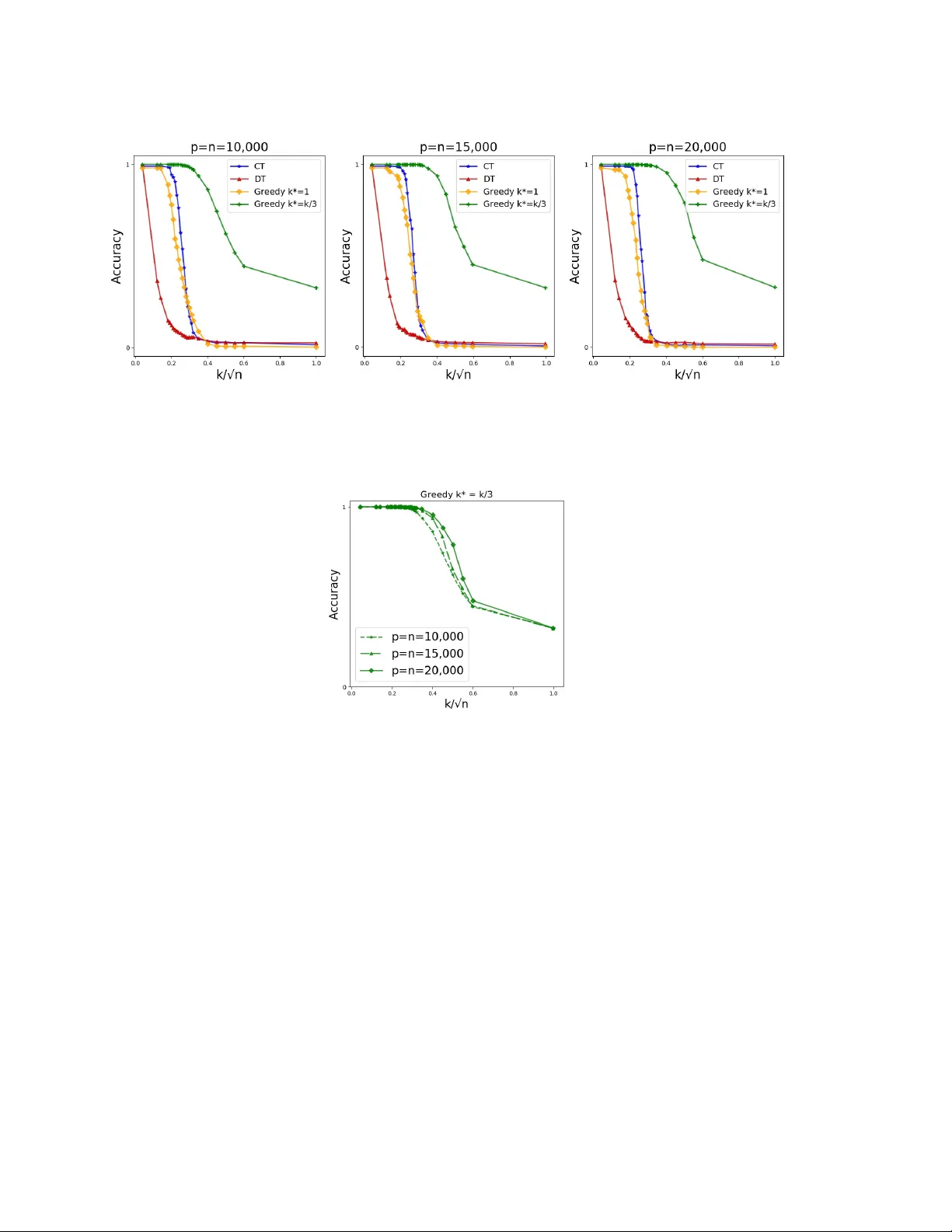
A greedy an ytime algorithm for sparse PCA Guy Holtzman ∗ Adam Soffer † Dan Vilenc hik ‡ F ebruary 13, 2020 Abstract The taxing computational effort that is in volv ed in solving some high-dimensional statistical problems, in particular problems in volving non-con v ex optimization, has pop- ularized the dev elopment and analysis of algorithms that run efficien tly (p olynomial- time) but with no general guarantee on statistical consistency . In light of the ever- increasing compute p o wer and decreasing costs, a more useful c haracterization of al- gorithms is b y their abilit y to calibrate the in v ested computational effort with v arious c haracteristics of the input at hand and with the av ailable computational resources. F or example, design an algorithm that alwa ys guarantees statistical consistency of its output b y increasing the running time as the SNR weak ens. W e prop ose a new greedy algorithm for the ` 0 -sparse PCA problem which supp orts the calibration principle. W e provide b oth a rigorous analysis of our algorithm in the spik ed co v ariance mo del, as w ell as sim ulation results and comparison with other existing metho ds. Our findings show that our algorithm recov ers the spik e in SNR regimes where all p olynomial-time algorithms fail while running in a reasonable parallel-time on a cluster. 1 In tro duction Principal comp onen ts analysis (PCA) is the mainsta y of mo dern mac hine learning and statistical inference, with a wide range of applications inv olving m ultiv ariate data, in b oth science and engineering [ And84 , Jol02 ]. The application of PCA to high-dimensional data, where features are plentiful (large p ) but samples are relativ ely scarce (small n ) suffers from t wo ma jor limitations: (1) the principal comp onen ts are typically a linear combination of all features, whic h hinders their interpretation and subsequent use; and (2) while PCA is consistent in the classical setting ( p is fixed and n go es to infinity) [ And84 , Mui82 ], it is generally inconsistent in high-dimensions [ Joh01 , Pau07 , BL08 , Nad08 , JL09 ]. This phenomenon is more generally known as the “Curse of Dimensionality” [ Don00 ]. The lack of consistency and interpretabilit y in the high-dimensional setting encouraged researc hers to design regularized estimation schemes, where additional structural informa- tion on the parameters describing the statistical mo dels is assumed an d in particular v arious ∗ Ben-Gurion Unv ersit y of the Negev, Beer-Shev a, Israel † Ben-Gurion Unv ersit y of the Negev, Beer-Shev a, Israel ‡ Ben-Gurion Unv ersit y of the Negev, Beer-Shev a, Israel. 1 sparsit y assumptions. One such p opular mo del is the ` 0 -sparse PCA, or k -sparse PCA as w e call it from now on. The input to k -sparse PCA is a pair ( X , k ), where X is an n × p design matrix and k the desired sparsity level. The goal is to find a unit vector v that has at most k non-zero entries, a k -sparse vector, such that the v ariance of X in v ’s direction is maximal. While standard (non-restricted) PCA can b e efficien tly solved by computing the eigen- v ectors of a symmetric matrix, its k -sparse v arian t has a discrete com binatorial fla vor that turns it NP-hard [ Nat95 ]. Nev ertheless, computationally efficient heuristics for k -sparse PCA w ere prop osed and analyzed under v arious assumptions on the distribution of X and the parameters n, p and k , e.g. [ JL09 , A W09 , dEGJL04 , KNV15 , DM16 ]. The performance of all the aforecited algorithms features a rather undesirable phase- transition behavior (at least on the benchmark distribution that was studied in eac h pap er). Eac h algorithm A performs w ell up to a certain SNR threshold τ A , and its p erformance deteriorates as the SNR drops b elo w τ A (w e formalize the notion of signal-to-noise-ratio in Section 3 ). Such a threshold b eha vior is exp ected in a w orse-case setting, as the problem is NP-hard. Ho w ev er, the results of [ BR13b , BR13a , KNV15 , BB19 ] suggest that the threshold b eha vior might p ersist ev en in the av erage-case setting, as long as the algorithms b elong to the p olynomial-time family . Throughout w e let v ∗ ∈ R p denote the solution of the k -sparse PCA problem and I ∗ ⊆ { 1 , . . . , p } the supp ort of v ∗ . W e denote by Σ = 1 n X T X the sample co v ariance matrix, assuming X is cen tered. In what follows, w e consider the equiv alen t problem of finding the supp ort set I ∗ rather than v ∗ . 2 Our con tribution An ytime algorithms provide the abilit y to achiev e results of b etter qualit y in return for running time [ Zil96 ]. W e implemen t this philosophy in the context of the sparse PCA problem. W e prop ose a new algorithm that consists of a tunable parameter that allo ws increasing the running time as the SNR weak ens. Th us the algorithm maintains a steady success rate and av oids the aforemen tioned threshold b eha vior. If necessary , the algorithm in vests sup er p olynomial-time. T o understand our algorithm, it will b e conv enien t to reformulate k -sparse PCA as follo ws. F or a fixed symmetric matrix Σ ∈ R p × p , define f (Σ) λ 1 : 2 { 1 ,...,p } → R by f (Σ) λ 1 ( S ) = λ 1 (Σ S ) , where Σ S is the principal submatrix of Σ corresp onding to the v ariables in S and λ 1 is its largest eigen v alue. F or simplicity we abbreviate f (Σ) λ 1 b y f λ 1 as Σ is alw ays clear from the context. The k -sparse PCA problem is the solution of I ∗ = argmax S ⊆{ 1 ,...,p } |S | = k f λ 1 ( S ) . (2.1) Our algorithm is comp osed of tw o routines. The first, which we call GreedySprasePCA, receiv es a real v alued function f : 2 { 1 ,...,p } → R (for example f λ 1 ), a seed S ∗ ⊆ { 1 , . . . , p } 2 of size k ∗ ≤ k , and a solution size k . It greedily completes S ∗ to a candidate solution of k -sparse PCA. GreedySPCA( f , S ∗ , k ) : 1: k ∗ ← |S ∗ | 2: for all i ∈ { 1 , . . . , p } \ S ∗ do 3: a i ← f ( S ∗ ∪ { i } ) 4: end for 5: sort the a i ’s as a i 1 ≥ a i 2 ≥ ... ≥ a i p − k ∗ 6: return S ∗ ∪ { i 1 , . . . , i k − k ∗ } The next routine, SeedSparsePCA (SSPCA for short) enumerates o ver all p ossible seeds of a given size k ∗ , completes eac h one using GreedySPCA, and returns the “b est” solution. SSPCA ( f 1 , f 2 , k , k ∗ ) : 1: for all seeds S ∗ ⊆ { 1 , . . . , p } of size k ∗ do 2: S ( S ∗ ) ← GreedySPCA( f 1 , S ∗ , k ) 3: end for 4: return argmax S ∗ f 2 ( S ( S ∗ ) ) Note that SSPCA is actually a family of algorithms, depending on the h yp er-parameters f 1 , f 2 . W e shortly discuss the choice of these parameters. The running time of SSPCA is  p k ∗  O ( pk ∗ + k log k ). By v arying k ∗ one obtains a hierarc hy of algorithms, whic h for our c hoice of f 1 , f 2 ranges from Diagonal Thresholding [ JL09 ] (for k ∗ = 0) up to the naiv e exhaustive search (for k ∗ = k ). The hierarc hy realizes the any time principle. Another attractive feature of SSPCA, esp ecially for practitioners, is the fact that it is completely white-b ox with only one simple tunable parameter, k ∗ . F urthermore, SSPCA can easily be parallelized and run in a multi-core cluster envir onment. The co de we share is written in that wa y . The following tw o conditions are sufficient for SSPCA( f 1 , f 2 , k , k ∗ ) to reco v er at least ( δ − ξ )-fraction of I ∗ , for tw o n um b ers δ, ξ ∈ [0 , 1] . C1. There exists a golden se e d S ∗ of size k ∗ suc h that GreedySPCA( f 1 , S ∗ , k ) outputs a set I satisfying |I ∩ I ∗ | ≥ δ k . C2. Σ is ξ -sep ar able with resp ect to f 2 . Namely , for every tw o sets I , J of size k , if |I ∩ I ∗ | − |J ∩ I ∗ | ≥ ξ k then f 2 ( I ) > f 2 ( J ). F or C1 and C2 to b e meaningful, one should think of golden seeds with δ close to 1, and f 2 -separabilit y with ξ close to 0. Prop osition 4.1 formally asserts the sufficiency of these conditions. 3 Figure 1: The plot p ortrays the accuracy a v eraged ov er 25 executions in the uniform un biased spik ed co v ariance mo del (USPCA), parametrized to suit a w eak SNR regime ( n = p = 1000 , k = 8 , β = 0 . 5). The compared algorithms are SSPCA with v arious seed sizes, Diagonal Thresholding (DT) [ JL09 ], Co v ariance Thresholding (CT) [ BL08 ], LARS regression [ ZHT06 ] and a naive exhaustiv e searc h that w as allow ed the same running time as SSPCA with k ∗ = 3. F ull details of the executions are giv en in Section 8 . The av erage running time is stated b elow each algorithm name. The reported running time of SSPCA and the preempted exhaustiv e search is a parallel-time using 90 Intel Xeon Processor E7-4850 v4 (40M Cache, 2.10 GHz) cores. The definition of k -sparse PCA in Eq. ( 2.1 ) suggests the c hoice f 2 = f λ 1 , whic h is indeed what w e chose. F or the rigorous analysis, we chose f 1 = f av g ( S ) = 1 |S | P i,j ∈S Σ i,j , namely the av erage ro w sum in Σ S . Note that for ev ery S , f λ 1 ( S ) ≥ f av g ( S ) by plugging the c haracteristic vector of S in the Ra yleigh-quotient definition of λ 1 . In the simulation part, w e exp erimented with other functions as well. Details in Section 8 . W e analyze SSPCA rigorously in the well-kno wn spik ed cov ariance model, which is formally defined in Section 3 . Theorem 4.2 establishes the scaling of k ∗ as a function of the parameters ( n, p, k ), for which condition C1 holds with δ = 1. Theorem 4.3 and Corollary 4.4 explicate the gap parameter ξ in condition C2 as a function of ( n, p, k ), from which the regime where ξ = o (1) is obtained. T ogether they guarantee the recov ery of (1 − o (1))- fraction of I ∗ , up to the information limit. Our results are asymptotic, namely , they hold with probabilit y (w.p.) tending to 1 as the parameters of the problem ( n, p, k ) go to infinit y . The probabilit y is taken only o ver the choice of the design matrix X . Figure 1 summarizes sim ulations that sho w how our approac h implements the an ytime paradigm: increasing k ∗ (and subsequently the running time of SSPCA) translates to the desired increase in the solution quality . W e further compared the p erformance of SSPCA when allo wed “p olynomial-time” ( k ∗ = 1 , 2) to three p opular p olynomial-time algorithms. Figure 1 sho ws that SSPCA is b etter than all three. Finally , w e show that SSPCA with k ∗ = 3 outperforms the naiv e exhaustiv e search when b oth are running for the same amoun t of time. This suggests the following rule-of-thum b: Rather than trying to nail do wn I ∗ b y going ov er as man y sets of size k as p ossible using time budget T , w e suggest to skim 4 through a larger n umber of smaller sets of size k ∗ < k , completing eac h one in a greedy manner (GreedySPCA). Finally , let us men tion that indep enden tly of this result, a different anytime algorithm for k -sparse PCA was obtained in [ DKWB19 ]. The algorithm also emplo ys a controlled exhaustiv e search part, but the ov erall algorithmic approach is differen t. The algorithm w as rigorously analyzed in the spiked cov ariance mo del as w ell and, in terestingly , both algorithms hav e the same asymptotic run-time, namely the same requirement on the seed size. In fact, [ DKWB19 ] pro vide evidence that this requiremen t is tight. 3 The Spik ed Cov ariance Mo del The spiked cov ariance mo del was suggested by Johnstone in 2001 [ Joh01 ] to mo del a com- bined effect of a lo w-dimensional signal buried in high-dimensional noise. In this pap er, we consider the Gaussian case with a single spike, where the p opulation cov ariance matrix is Σ = β v ∗ v ∗ T + I p . The parameter β ≥ 0 is the signal strength, v ∗ ∈ R p is the plan ted spik e assumed to b e a k -sparse unit-length v ector. The algorithmic task is to reco ver I ∗ , the supp ort of v ∗ , given n iid samples x 1 , . . . , x n from N (0 , Σ). The SNR is gov erned b oth b y β and k . The larger β and the smaller k the stronger the SNR and the easier the task. There is an extensiv e literature on efficient algorithms for sparse PCA, which w ere rigorously analyzed under v arious v ariants of the mo del just describ ed, e.g. [ A W09 , CMW13 , SSM13 , JL09 , DM16 , KNV15 , WBS16 ]. All these algorithms succeed in the regime where the sparsit y lev el satisfies k = ˜ O ( p β 2 n ) (w e use the ˜ O ( · ) notation in the common w ay , namely logarithmic factors are ignored). The b est sparsit y asymptotically is achiev ed for example by Cov ariance Thresholding (CT) [ DM16 ], remaining consistent up to k 0  p β 2 n (the notation f  g stands for f /g → c for some constan t c > 0). It was further shown that under the plan ted clique hardness assumption there is no p olynomial-time algorithm that asymptotically beats k 0 [ BB19 , BR13b , BR13a ]. Ev en without the plan ted clique assumption, [ KNV15 ] show that the SDP relaxation suggested b y [ dEGJL04 ] and analyzed by [ A W09 ], fails to recov er v ∗ b ey ond k 0 . The threshold k 0 is commonly referred to as the computational threshold, which we denote from no w on b y k comp . W e informally call the regime k >> k comp the weak SNR regime, and k ≤ k comp the strong SNR regime. Finally , an information-limit w as pro v en for k ≥ k inf o  β 2 n/ log p [ A W09 , BR13b , CMW15 , WBS14 ], and a matching algorithmic result for the naiv e exhaustive search [ VL12 , CMW13 , BR13a , BBH18 ]. While the b oundaries b et ween the different SNR regimes are well understo o d, at least asymptotically , the following question remains op en: Question: what is the (minimal) c omputational c omplexity r e quir e d to find the supp ort of v ∗ in the we ak SNR r e gime, namely when k comp ≤ k ≤ k inf o ? The analysis of SSPCA in the next sections provides an answer. 5 4 Results Our results refer to the follo wing choice of hyper-parameters for SSPCA: f 1 = f av g ( S ) = 1 |S | X i,j ∈S Σ i,j , f 2 = f λ 1 ( S ) = λ 1 (Σ S ) . F urthermore, w e assume the uniform biase d sp arse PCA mo del (UBSPCA), namely non-zero en tries of v ∗ are all equal to 1 / √ k . In the simulation part w e lift the same-sign restriction and use the uniform unbiase d sp arse PCA mo del (USPCA), where entries equal ± 1 / √ k . The next prop osition asserts the sufficiency of conditions C1, C2. Prop osition 4.1 ( δ, ξ − Sufficient Conditions) . If Σ is ξ -sep ar able (Condition C2) and ther e exists a golden se e d S 0 of size k ∗ such that Gr e e dySPCA ( X, k , S 0 ) outputs a set I 0 satisfying |I 0 ∩ I ∗ | ≥ δ k (Condition C1) then SSPCA outputs a set I satisfying |I ∩ I ∗ | ≥ ( δ − ξ ) k . The proof of Prop osition 4.1 is giv en in Section 5 . Our next theorem establishes the scaling of k ∗ for the existence of a seed from which I ∗ is recov ered exactly (condition C1 with δ = 1). Theorem 4.2 (Golden seed) . L et Σ b e distribute d ac c or ding to the UBSPCA mo del. As- sume that p/n → c ≥ 0 , and k ≤ n · min { β 2 ,β } C log n for a sufficiently lar ge universal c onstant C . If k ∗ ≥ j C k 2 log n β 2 n k (4.1) then w.p. tending to 1 as ( n, p, k ) → ∞ ther e exists a se e d S ∗ ⊆ I ∗ of size at most k ∗ for which the output of Gr e e dySPCA ( f av g , S ∗ , k ) is I ∗ . Theorem 4.2 is pro ven in Section 6 . The next theorem pro vides a general sp ectral separabilit y property of spik ed co v ariance matrices. It implies condition C2 as an immediate corollary . Theorem 4.3 (Sp ectral Separation) . L et Σ b e distribute d ac c or ding to the UBSPCA mo del with p/n → c > 0 . Set Γ = C  (1+ β ) k log n n  0 . 5 for a suitably chosen c onstant C . With pr ob ability tending to 1 as ( n, p, k ) → ∞ , for every δ ∈ [0 , 1] and for every set I ⊆ { 1 , . . . , p } of size k that satisfies |I ∩ I ∗ | = δ k , λ 1 (Σ I ) ∈  1 + δ β − Γ , 1 + δ β + Γ + β k  . Corollary 4.4 (Condition C2) . Under the c onditions of The or em 4.3 , for every two sets I , J of size k , if |I ∩ I ∗ | − |J ∩ I ∗ | > ξ k then λ 1 (Σ I ) > λ 1 (Σ J ) , for ξ that satisfies ξ = 1 k + O s (1 + β ) k k inf o ! , (4.2) wher e k inf o  β 2 n/ log p was define d in Se ction. 3 6 Theorem 4.3 is pro ven in Section 7 and Corollary 4.4 is prov en in Section 7.4 . Corollary 4.4 with I = I ∗ w as already pro ven for example in [ VL12 , CMW13 , BR13a , BBH18 ] and in a more general sparse PCA mo del. Corollary 4.4 adds that even if the seed suffices to reco ver only part of I ∗ , which might as well b e the case in practice (finite problem size), SSPCA will nev ertheless pick up this information. This p oin t is demonstrated in Figure 1 , where all executions of SSPCA end up with partial recov ery . The next theorem concludes our result and is an immediate corollary of all the statemen ts in this section. Theorem 4.5. Under the c onditions of The or em 4.2 , if k ∗ satisfies the lower b ound in Eq. ( 4.1 ) , then w.p. tending to 1 as ( n, p, k ) → ∞ , SSPCA ( f av g , f λ 1 , k , k ∗ ) r e c overs at le ast (1 − O ( √ α ) − 1 /k ) -fr action of I ∗ , wher e α = (1 + β ) k /k inf o . F or example, in the regime where DT and SDP fully recov er I ∗ , i.e. k = O ( k comp / √ log p ), SSPCA requires a seed of size 0 to recov er I ∗ and runs in time O ( p log p ). When k  k comp the seed size is k ∗ = O (log n ) and the running time is quasi-p olynomial, p O (log n ) . Sim ula- tions suggest that up to the computational threshold, ev en for a fairly large problem size ( n = p = 20 , 000), it suffices to c ho ose k ∗ = 1 to recov er I ∗ exactly (see Figure 2 ). In the w eak SNR regime, i.e. k = n 0 . 5+ ε , the seed size scales as n 2 ε log n . This means that the computational effort is exp { n 2 ε log n } , which is exp onen tial in ( k / √ n ) 2 (square the excess ab o ve the computational threshold) rather than in k itself (the naiv e exhaustive search approac h). The results in [ DKWB19 ][Thm 2.14] provide rigorous evidence that the exact scaling that we obtained for k ∗ in Eq. ( 4.1 ) is asymptotically optimal. Sim ulation (Section 8 ) suggests that SSPCA succeeds also when the UBSPCA assump- tion is relaxed, namely the same-sign assumption is lifted. In this case, the b est performance is ac hieved when the hyper-parameter f av g is replaced with f ` 1 , which is the av erage row ` 1 -norm rather than the av erage ro w sum. The parameter f 2 = f λ 1 remains the same. 5 Pro of of Prop osition 4.1 Supp ose by contradiction that conditions C1 and C2 hold but SSPCA outputs a set J for whic h |J ∩ I ∗ | < ( δ − ξ ) k . Consider a point in the execution of SSPCA where a golden seed S 0 is explored. By Condition C1, GreedySPCA completes S 0 to a set I satisfying |I ∩ I ∗ | ≥ δ k . The latter together with the contradiction assumption giv e |I ∩ I ∗ | − |J ∩ I ∗ | > δ k − ( δ − ξ ) k = ξ k . In this case C2 guarantees that λ 1 (Σ I ) > λ 1 (Σ J ). Therefore the last line of SSPCA ensures that J cannot b e the output of the algorithm. 6 Pro of of Theorem 4.2 F or con venience, let us assumes w.l.o.g. that the supp ort of v ∗ is the first k v ariables, namely I ∗ = { 1 , . . . , k } . Our candidate for a golden seed is any subset S ∗ of I ∗ . F or concreteness we fix S ∗ = { 1 , . . . , k ∗ } . W e show that when GreedySPCA is called with this 7 subset, then the k − k ∗ v ariables that it adds to S ∗ in line 6, all b elong to { 1 , . . . , k } , thus outputting I ∗ . W e b egin by writing the distribution of the i th sample from N (0 , β v ∗ v ∗ T + I p ) explicitly as x i = p β u i v ∗ + ξ i , (6.1) where ξ i ∈ R p is a noise vector whose entries are all i.i.d. N (0 , 1), and u i ∼ N (0 , 1). F urthermore, all the u i ’s and ξ i ’s are indep endent of each other. By the greedy rule in line 3 of GreedySPCA, the k − k ∗ v ariables in { 1 , . . . , p } \ S ∗ that will b e chosen are those with largest v alue of f av g ( S ∗ ∪ { i } ). W e rewrite f av g ( S ∗ ∪ { i } ) as f av g ( S ∗ ∪ { i } ) = 1 k ∗ +1 X s,t ∈S ∗ ∪{ i } Σ s,t = k ∗ k ∗ +1 f av g ( S ∗ ) + 2 k ∗ +1 X s ∈S ∗ Σ is ! | {z } c i ( S ∗ ) + 1 k ∗ +1 Σ ii := (6.2) := k ∗ k ∗ +1 f av g ( S ∗ ) + 1 k ∗ +1 (2 c i ( S ∗ ) + Σ ii ) . The only part in Eq. ( 6.2 ) that dep ends on i is its total cov ariance with S ∗ (whic h we denote by c i ), and its v ariance Σ ii . In high lev el, the algorithm succeeds since c i is muc h bigger than c j for all pairs i ∈ I ∗ , j / ∈ I ∗ . W e no w turn to make this argumen t formal. Lemma 6.1. Under the c onditions of The or em 4.2 , for a fixe d S ∗ ⊆ I ∗ of size k ∗ , w.p. at le ast 1 − 1 /n , every i ∈ I ∗ satisfies c i ≥ 0 . 4 β k ∗ /k . Lemma 6.2. Under the c onditions of The or em 4.2 , for a fixe d S ∗ ⊆ I ∗ of size k ∗ , w.p. at le ast 1 − 1 /n , every j / ∈ I ∗ satisfies c j ≤ 0 . 3 β k ∗ /k . Lemma 6.3. Under the c onditions of The or em 4.2 , with pr ob ability at le ast 1 − 1 /n , for every i ∈ I ∗ , j / ∈ I ∗ , Σ j j − Σ ii ≤ 0 . 1 β k ∗ /k . W e use Lemmas 6.1 , 6.2 and 6.3 to complete the pro of of the theorem. Let ∆ ij = f av g ( S ∗ ∪ { i } ) − f av g ( S ∗ ∪ { j } ). T o pro ve that GreedySPCA outputs I ∗ w e need to show that ∆ ij > 0 for every i ∈ I ∗ , j / ∈ I ∗ . Using Lemmas 6.1 – 6.3 , w e hav e k · ∆ ij ≥ 2(0 . 4 β k ∗ /k − 0 . 3 β k ∗ /k ) − 0 . 1 β k ∗ /k ≥ 0 . 1 β k ∗ /k > 0. In the last inequality we assumed k ∗ ≥ 1. The case k ∗ = 0 corresp onds to the regime k = O ( k comp / √ log p ). In this regime the k largest diagonal entries b elong to I ∗ [ JL09 ]. Indeed, when k ∗ = 0 then f av g ( { i } ) is simply Σ ii , and GreedySPCA is no other than Diagonal Thresholding. W e turn to prov e Lemmas 6.1 – 6.3 . In the pro of we use the following t wo auxiliary facts. The first is a large deviation result for a Chi-square random v ariable. Lemma 6.4. ([ LM00 ]) L et X ∼ χ 2 n . F or al l x ≥ 0 , P r [ X ≥ n + 2 √ nx + x ] ≤ e − x , P r [ X ≤ n − 2 √ nx ] ≤ e − x . 8 The second fact records a well-kno wn argumen t ab out the inner-pro duct of tw o multi- v ariate Gaussians. Lemma 6.5. L et { x i , y i } n i =1 b e standar d i.i.d. Gaussian r andom variables. Then P n i =1 x i y i is distribute d like the pr o duct of two indep endent r andom variables k x k · ˜ y , wher e x = ( x 1 , . . . , x n ) , k x k 2 ∼ χ 2 n and ˜ y ∼ N (0 , 1) . Pr o of. F or every fixed realization of x , w e ha ve x i y i ∼ N (0 , x 2 i ) and by the indep endence of the y i ’s, n X i =1 x i y i ∼ N (0 , k x k 2 ) = k x k · N (0 , 1) := k x k · ˜ y . The lemma follows by observing that k x k 2 ∼ χ 2 n .  6.1 Pro of of Lemma 6.1 W e start by explicitly writing c i ( S ∗ ) from Eq. ( 6.2 ) for a fixed set S ∗ of size k ∗ . Let r ( i ) denote the i th ro w of the p × n design matrix X . F or every candidate i / ∈ S ∗ , c i ( S ∗ ) = X j ∈S ∗ Σ ij = 1 n X j ∈S ∗ r ( i ) · ( r ( j ) ) T = 1 n r ( i )   X j ∈S ∗ r ( j )   T . F ollowing the distribution rule of X giv en in Eq. ( 6.1 ), all en tries of the vector s = P j ∈S ∗ r ( j ) are i.i.d. with s ` ∼ p β u ` X j ∈S ∗ v ∗ j + √ k ∗ w ` , where u ` ∼ N (0 , 1) is defined in Eq. ( 6.1 ) and w ` ∼ N (0 , 1) indep enden tly of u ` ( √ k ∗ w ` is deriv ed from P j ∈S ∗ ( ξ ` ) j ). The pro duct r ( i ) s T is distributed as r ( i ) s T ∼ 1 n n X ` =1  p β u ` v ∗ i + y `    p β u `   X j ∈S ∗ v ∗ j   + √ k ∗ w `   (6.3) The v ariable y ` = ( ξ ` ) i ∼ N (0 , 1). W e rearrange the sum as four comp onents, corresp onding to the pure signal part, cross noise-signal and pure noise: n X ` =1 p β u ` v ∗ i · p β u ` X j ∈S ∗ v ∗ j = β k ∗ v ∗ i √ k n X ` =1 u 2 ` , (6.4) n X ` =1 p β u ` v ∗ i · √ k ∗ w ` = p β k ∗ v ∗ i n X ` =1 u ` w ` , (6.5) n X ` =1 y ` p β u ` X j ∈S ∗ v ∗ j = √ β k ∗ √ k n X ` =1 y ` u ` , (6.6) n X ` =1 y ` √ k ∗ w ` = √ k ∗ n X ` =1 y ` w ` . (6.7) 9 W e now b ound each term separately . T o lo wer b ound Eq. ( 6.4 ), we use the fact that P n ` =1 u 2 ` in Eq. ( 6.4 ) is distributed χ 2 n . The second inequality in Lemma 6.4 with x = 0 . 05 n giv es P r [ χ 2 n ≤ 0 . 8 n ] ≤ e − n/ 100 . Therefore, w.p. at least 1 − e − n/ 100 , 1 n ( 6.4 ) ≥ 0 . 8 β k ∗ /k (6.8) Mo ving to Eq. ( 6.5 ), according to Lemma 6.5 , the pro duct term in Eq. ( 6.5 ) is distributed as p χ 2 n N (0 , 1). F or 1 n ( 6.5 ) > 0 . 1 β k ∗ /k to hold, the following has to happ en, p χ 2 n |N (0 , 1) | > β n √ k ∗ 10 k = β n √ k ∗ 30 k √ log n · p 9 log n. Using standard tail-b ounds for Gaussians, P r [ |N (0 , 1) | > √ 9 log n ] ≤ n − 4 . Next w e b ound P r [ χ 2 n ≥ β 2 n 2 k ∗ / (900 k 2 log n )] . Substituting the v alue of k ∗ from Eq. ( 4.1 ) we hav e that β 2 n 2 k ∗ 900 k 2 log n ≥ β 2 n 2 900 k 2 log n · C k 2 log n β 2 n = C n/ 900 . Cho osing C ≥ 1800 for example and using Lemma 6.5 gives P r [ χ 2 n ≥ 2 n ] ≤ e − n/ 4 . T o conclude, w.p. at least 1 − n − 4 − e − n/ 4 w e get 1 n | ( 6.5 ) | ≤ 0 . 1 β k ∗ k (6.9) Mo ving to Eq. ( 6.6 ), according to Lemma 6.5 , the sum-pro duct term in Eq. ( 6.6 ) is distributed as p χ 2 n N (0 , 1). Using standard tail-b ounds for Gaussians, P r [ |N (0 , 1) | ≥ √ 6 log n ] ≤ 2 n − 3 , and according to Lemma 6.4 , P r [ χ 2 n ≥ 2 n ] ≤ e − n/ 4 . Therefore w.p. at least 1 − 2 n − 3 − e − n/ 4 w e get 1 n ( 6.6 ) ≤ 1 n √ β k ∗ √ k p 6 log n √ 2 n ≤ 0 . 1 β k ∗ k (6.10) The last inequality is true when k ≤ β n/ (1200 log n ), which holds b y our choice of k . Mo ving to Eq. ( 6.7 ), w e similarly hav e that w.p. at least 1 − 2 n − 3 − e − n/ 4 1 n ( 6.7 ) ≤ 1 n √ k ∗ p 6 log n √ 2 n ≤ 0 . 2 k ∗ β k . (6.11) The last inequality in Eq. ( 6.11 ) holds whenever k ∗ ≥ 200 k 2 log n/ ( β 2 n ), which is what Eq. ( 4.1 ) says. Finally , the lo w er b ound on k ∗ in Eq. ( 4.1 ) mak es sense as long as k ∗ ≤ k , whic h translates to requiring k ≤ β 2 n/ ( C log n ). T o conclude, w.p. at least 1 − 3 n − 3 , for a fixed i ∈ I ∗ , c i ≥ ( 6.8 ) − ( 6.9 ) − ( 6.10 ) − ( 6.11 ) ≥ 0 . 4 k ∗ β k . The lemma now follo ws from taking the union b ound o v er the k − k ∗ ≤ p indices in I ∗ \ S ∗ , together with the fact that p = O ( n ). 10 6.2 Pro of of Lemma 6.2 F or i / ∈ I ∗ the terms in Eq. ( 6.4 ) and ( 6.5 ) are 0 (b ecause v ∗ i = 0). The pro of of Lemma 6.2 is identical to the proof leading to the b ound on Eq. ( 6.6 ) giv en in Eq. ( 6.10 ) and to the b ound on Eq. ( 6.7 ) given in Eq. ( 6.11 ). A union b ound is then tak en ov er the at most p v ariables in { 1 , . . . , p } \ I ∗ . 6.3 Pro of of Lemma 6.3 F or j / ∈ I ∗ , the distribution of Σ j j ∼ χ 2 n n (F rom Eq. ( 6.3 )). Lemma 6.4 en tails that for a fixed j , w.p. at least 1 − n − 3 , Σ j j ≤ 1 + q 9 log n n . F or i ∈ I ∗ , Σ ii ∼ β k χ 2 n n + 2 √ β √ k N (0 , 1) p χ 2 n n + χ 2 n n Using Lemma 6.4 and standard tails on the Gaussian, w e obtain that w.p. at least 1 − O ( n − 3 ), Σ ii ≥ 1 + β k − q 36 log n n . Using the union b ound w e get that w.p. at least 1 − O ( n − 1 ), for every pair i ∈ I ∗ , j / ∈ I ∗ , Σ j j − Σ ii ≤ r 100 log n n − β k ≤ r 100 log n n ≤ 0 . 1 β k ∗ k . The last inequality holds if k ∗ ≥ √ L , where L is the low er b ound on k ∗ in Eq. ( 4.1 ). Ho wev er, k ∗ ≥ L implies k ∗ ≥ √ L since k ∗ is an integer. 7 Pro of of Theorem 4.3 W e prov e that w.p. tending to 1 as ( n, p, k ) → ∞ , for every set I ⊆ { 1 , . . . , p } of size k that satisfies |I ∩ I ∗ | = δ k , for ev ery δ ∈ [0 , 1]: λ 1 (Σ S ) ∈ [1 + δ β − (1 + 2 p β )Φ , 1 + δ β + (1 + 2 p β )Φ + β k ] , (7.1) Where Φ = q 8 k log n n . Fix a set I ⊆ { 1 , . . . , p } s.t. |I ∩ I ∗ | = δ k . The matrix Σ I can b e written as Σ I = N + S where N is comp osed of the noise part, Eq. ( 6.7 ), and S is comp osed of the signal and noise- signal cross terms, Eq. ( 6.4 )–( 6.6 ). N is easily seen to b e symmetric (in fact it follo ws a Wishart distribution), and therefore the matrix S = Σ I − N , the difference of t wo symmetric matrices, is symmetric as w ell. W eyl’s inequalit y , applicable for Hermitian matrices, implies that λ k ( N ) + λ 1 ( S ) ≤ λ 1 (Σ I ) ≤ λ 1 ( N ) + λ 1 ( S ) (7.2) 11 7.1 Bounding λ 1 ( N ) and λ k ( N ) The matrix N ∈ R k × k follo ws a Wishart distribution, and b y [ DS01 , Theorem I I.13], Pr[ λ 1 ( N ) ≥ (1 + p k /n + t ) 2 ∨ λ k ( N ) ≤ (1 − p k /n − t ) 2 ] ≤ e − nt 2 / 2 . Plugging in t = p 6 k log n/n w e obtain that w.p. at least 1 − n − 3 k , λ 1 ( N ) ≤ 1 + r k n + r 6 k log n n ! 2 ≤ 1 + r 8 k log n n = 1 + Φ . (7.3) and similarly , λ k ( N ) ≥ 1 − Φ . (7.4) T aking the union b ound o ver all  p k  ≤ p k p ossible sub-matrices N , the b ounds hold w.p. at least 1 − n − 3 k p k ≥ 1 − n − 1 . 7.2 Upp er Bounding λ 1 ( S ) Recall the parameters u = ( u 1 , . . . , u n ) and ξ i from definition of the single-spike distribution giv en in Eq. ( 6.1 ). W e start with a certain prop ert y of Σ that we require during the proof of the upp er and lo wer b ound on λ 1 ( S ). W e say that Σ is typic al if k u k 2 ≤ n + 6 √ n log n and if ( ξ 1 ) i ≤ 2 √ log n for every i = 1 , . . . , p . Lemmas 6.4 and 6.5 guarantee that Σ is typical w.p. at least 1 − n − 1 . In what follo ws we condition on this fact. T o upp er b ound the largest eigenv alue of S w e use Gershgorin’s circle theorem, which sa ys that ev ery eigenv alue λ of an n × n matrix A satisfies at least one of the n inequalities for i = 1 , . . . , n , | λ − A ii | ≤ X j 6 = i | A ij | . (7.5) Eac h inequalit y defines a Gershgorin’s disc, and ev ery λ b elongs to at least one disc. W e next show that all discs are almost iden tical, and ev aluate their center and radius. Decomp ose eac h en try S ij according to the three sums Eq. ( 6.4 )-( 6.6 ) (plugging k ∗ = 1). T o b ound the sums in Eq.( 6.5 ) and ( 6.6 ) we note that b oth inv olv e the term u ` , whic h do es not dep end on i or j . Therefore w e may rotate the distribution to p oin t in the direction of u . According to Lemma 6.5 , the sum-pro duct ( 6.5 ) is then distributed k u k · ( ξ 1 ) i and Eq.( 6.6 ) is distributed k u k · ( ξ 1 ) j . Using the fact that Σ is typical w e obtain the follo wing b ounds: 1 n | ( 6.5 ) | ∼ 1 n p β v ∗ i k u k| ( ξ 1 ) j | ≤ r 8 β log n nk . Similarly 1 n | ( 6.6 ) | ≤ r 8 β log n nk , 1 n | ( 6.4 ) | = 1 ± r 36 log n n ! β k . Putting everything together, and letting δ i = 1 if i ∈ I ∗ and 0 otherwise, if Σ is typical then for every i, j ∈ I , S ij = δ i δ j β k + ∆ ij , | ∆ ij | ≤ ∆ := r 36 β log n nk . (7.6) 12 T o b ound the radius of the i th disc, P j | S ij | , w e need to accoun t for |I ∩ I ∗ | = δ k indices j ∈ I ∗ and (1 − δ ) k indices j / ∈ I ∗ . Plugging ( 7.6 ) in ( 7.5 ), we obtain that | λ − S ii | ≤ δ k  β k + ∆  + (1 − δ ) k · ∆ = δ β + ∆ k . Rearranging w e get λ 1 ( S ) ≤ S ii + δ β + ∆ k ≤ β k + ∆ + δ β + ∆ k ≤ δ β +  β k + 2∆ k  . (7.7) 7.3 Lo w er Bounding λ 1 ( S ) T o low er b ound the largest eigenv alue of S we use the Rayleigh quotient definition, namely λ 1 ( S ) is the argmax of x T S x ov er all unit vectors x ∈ R k . In particular, for x 0 = ( δ k ) − 0 . 5 1 I ∩I ∗ ( 1 Q is the characteristic v ector of a set Q ), the v alue of x T 0 S x 0 is a low er b ound on λ 1 ( S ). The latter is simply the av erage row sum in the δ k × δ k submatrix S I ∩I ∗ . If Σ is typical, then according to Eq. ( 7.6 ), λ 1 ( S ) ≥ δ k ·  β k − ∆  ≥ δ β − ∆ k . (7.8) T o conclude the proof of the theorem, note that ∆ k ≤ 3 √ β Φ. Putting Equations ( 7.3 ),( 7.4 ),( 7.7 ),( 7.8 ) together, we get that w.p. at least 1 − 2 n − 1 , λ 1 (Σ S ) ∈ [1 + δ β − (1 + 3 p β )Φ , 1 + δ β + (1 + 3 p β )Φ + β k ] . 7.4 Pro of of Corollary 4.4 T ake I , J ⊆ { 1 , . . . , p } that satisfy |I ∩ I ∗ | = δ 1 > δ 2 = |J ∩ I ∗ | . According to Theorem 4.3 , for λ 1 (Σ I ) > λ 1 (Σ J ) to hold, it suffices to require 1 + δ 2 β + β k + Γ < 1 + δ 1 β − Γ . Rearranging w e get, 2Γ β + 1 k < δ 1 − δ 2 := ξ . The corollary follows immediately from the definition of Γ and k inf o . 8 Sim ulations In this section, we ev aluate the p erformance of SSPCA b oth in the strong and weak SNR regimes. The definition of k comp in Section 3 (the boundary betw een the t w o regimes) is asymptotic and cannot b e used directly in simulation. Instead, w e let the empirical success rate of Cov ariance Thresholding (abbreviated CT) define regime b oundaries. The following p oin ts summarize the w ay we ran simulations: 13 • W e sample from the uniform unbiase d sparse PCA distribution (UNBSPCA), where v ∗ =  ± 1 √ k , . . . , ± 1 √ k , 0 , . . . , 0  . The signs of non-zero entries are randomly chosen. Accordingly , we change the c hoice of f 1 in GreedySPCA from f av g to f ` 1 , whic h measures the ` 1 norm of Σ S ∗ ∪{ i } , rather than the sum. F urthermore, in the weak SNR regime, it mak es sense to ignore the diagonal of Σ. Therefore w e only use c i from Eq. ( 6.2 ) to choose i , with ` 1 norm. • W e k eep p = n and fix β = 0 . 5. The choice of 0 . 5 is somewhat arbitrary and an y v alue b elo w p p/n = 1 is suitable. When β exceeds p p/n the problem is computationally easy for all k up to the information limit [ KNV15 ][Thm 1.1]. • The suc c ess r ate of an algorithm on a giv en input is defined to b e 1 k |I ∩ I ∗ | , where I ⊆ { 1 , . . . , p } is the algorithm’s guess of v ∗ ’s supp ort. • The algorithm DT has no tunable parameters – it simply returns the indices of the k largest diagonal en tries. The performance of CT, on the other hand, depends crucially on the c hosen threshold. When running CT we lo op ov er 50 thresholds, the empirical p ercen tiles of the off-diagonal en tries of the input cov ariance matrix. W e choose the b est result as CT’s output. • F ormally , the output of CT is a v ector (a guess for v ∗ ). W e con v ert the vector to a set I b y taking the indices of the k largest entries in absolute v alue. • W e compared SSPCA against the well-kno wn sparse PCA algorithm described in [ ZHT06 ]. This algorithm casts PCA as a regression problem and uses b oth ridge and lasso p enalties. LARS [ EHJT04 ] is then used to obtain the optimal solution. W e ran Python’s implementation of this algorithm using a grid search for the ridge and lasso p enalties in the rectangle [0 , 2] × [0 , 2], discretized to 100 equidistan t p oints. The algorithm is in mo dule sklearn.decomposition.SparsePCA [ PV G + 11 ]. Figure 1 compares the p erformance of all aforemen tioned algorithms in a certain weak SNR configuration, n = p = 1000 , k = 8 , β = 0 . 5. Among the p olynomial-time algorithms (w e include in this category SSPCA with k ∗ = 1 , 2), SSPCA with k ∗ = 2 p erforms best. When running for sup er p olynomial-time, SSPCA with k ∗ = 3 is sup erior to the naiv e exhaustiv e searc h, when b oth are giv en the same time budget T (3 parallel-hours on 90 cores). Our next exp eriment demonstrates the existence of golden seeds in the weak SNR regime. The empirical b oundary of the strong/w eak SNR regime is c harted b y the success rate curv e of CT. Figure 2 shows the p erformance ( y -axis) of CT as k increases. Three configurations are plotted n = p = 10 , 000 , 15 , 000 , 20 , 000. The x -axis is scaled by √ n to defuse the dep endence on n . Indeed all three CT lines ov erlap as exp ected (due to scaling), and the phase transition to the hard regime o ccurs when k is in the window [0 . 2 √ n, 0 . 3 √ n ]. The plot also includes the performance of DT, lagging behind, and GreedySPCA initialized once with a seed of size k ∗ = 1 and second with k ∗ = k / 3. In b oth cases the seed is a random subset of I ∗ . As eviden t from Figure 2 , the p erformance of GreedySPCA with seeds of size k ∗ = 1 is similar to CT. This is somewhat surprising when comparing to the asymptotic low er b ound 14 Figure 2: The success rate of DT, CT and GreedySPCA as a function of k . Every p oin t is an av erage of 25 executions, with n = p samples. GreedySPCA was initialized with k ∗ = 1 or k ∗ = k / 3 random entries from I ∗ . Figure 3: The success rate of GreedySPCA when initialized with k ∗ = k / 3 random entries from I ∗ . Lines are non-o v erlapping due to under-scaling on the x -axis. giv en b y Eq. ( 4.1 ), whic h w ould be of order log n at the computational threshold k comp . The righ t-most (green) line in Figure 2 extends with an accuracy of roughly 100% into the weak SNR regime, thus showing the existence of golden seeds in that regime. Another cue that w e are indeed in the w eak SNR regime is the fact that the lines in Figure 3 corresp onding to different input sizes do not ov erlap, suggesting that the scaling of the x -axis is to o small. 9 Discussion In this pap er, we presented a family of an ytime algorithms for the k -sparse PCA problem, whic h follo w the same simple white-b o x greedy template that we called GreedySPCA and SSPCA. GreedySPCA p erforms a bulk greedy c hoice, and instead we could hav e gro wn the so- lution iteratively , adding in iteration r = 1 , . . . , k − k ∗ the v ariable i r whic h maximizes 15 f 1 ( S ∗ ∪ { i 1 , . . . , i r − 1 } ). The iterativ e v ariant is exactly the w ell-known greedy algorithm of Nemhauser, W olsey and Fisher, whic h w as prop osed for sub-mo dular function optimiza- tion [ NWF78 ]. The only difference is that Nemhauser et al. start with an empt y seed. Nemhauser et al. pro ved that if f 1 is sub-modular and monotone, then the iterativ e greedy algorithm finds a solution which is a (1 − 1 e )-appro ximation of the optim um. Hence it is tempting to run the iterative greedy with f 1 = f λ 1 and no seed. Ho w ever, even if f λ 1 is monotone and sub-modular, the (1 − 1 e )-appro ximation ratio is useless in man y cases, as the guaran teed v alue is lo wer than a random solution (see Theorem 4.3 ). Our pro of sho ws that GreedySPCA recov ers I ∗ exactly when called with the righ t seed without the sub-mo dularit y assumption on f 1 . Sim ulations that we ran in the spik ed cov ariance mo del with the iterative version (with seed) resulted in v ery similar p erformance compared to the bulk version. Similarly , using f λ 1 instead of f ` 1 in GreedySPCA did not incur impro v ement. Ac kno wledgment W e thank Jonathan Rosen blatt for allowing us to use his cluster, and for his patient technical supp ort. References [And84] T. Anderson. A n intr o duction to multivariate statistic al analysis . Wiley series in probabilit y and mathematical statistics. Wiley , 2nd edition, 1984. [A W09] A. Amini and M. W ain wright. High dimensional analysis of semidefinite relaxations for sparse principal comp onent analysis. A nnals of Statistics , 37(5B):2877–2921, 2009. doi:10.1214/08- AOS664 . [BB19] M. Brennan and G. Bresler. Optimal av erage-case reductions to sparse p ca: F rom weak assumptions to strong hardness. In COL T , 02 2019. [BBH18] M. Brennan, G. Bresler, and W. Huleihel. Reducibility and computational low er b ounds for problems with planted sparse structure. In Pr o c e e dings of the 31st Confer enc e On L e arning The ory , volume 75 of Pr o c e e dings of Machine L e arning R ese ar ch , pages 48–166. PMLR, 06–09 Jul 2018. [BL08] J. Bic kel and E. Levina. Regularized estimation of large cov ariance matrices. A nnals of Statistics , 36:199–227, 2008. doi:10.1214/ 009053607000000758 . [BR13a] Q. Berthet and P . Rigollet. Complexity theoretic low er bounds for sparse principal comp onent detection. In COL T , pages 1046–1066, 2013. arXiv: 1304.0828 . 16 [BR13b] Q. Berthet and P . Rigollet. Optimal detection of sparse principal comp onen ts in high dimension. A nnals of Statistics , 41(4):1780–1815, 08 2013. doi:10. 1214/13- AOS1127 . [CMW13] T. Cai, Z. Ma, and Y. W u. Sparse PCA: Optimal rates and adaptiv e esti- mation. The Annals of Statistics , 41(6):3074–3110, 2013. doi:10.1214/ 13- AOS1178 . [CMW15] T. Cai, Z. Ma, and Y. W u. Optimal estimation and rank detection for sparse spik ed cov ariance matrices. Pr ob ability The ory and R elate d Fields , 161(3-4):781– 815, 4 2015. doi:10.1007/s00440- 014- 0562- z . [dEGJL04] A. d’Aspremont, L. El-Ghaoui, M. Jordan, and G. Lanckriet. A direct formula- tion for sparse PCA using semidefinite programming. SIAM R eview , 49(3):434– 448, 2004. doi:10.1137/050645506 . [DKWB19] Y. Ding, D. Kunisky , A. S. W ein, and A. S. Bandeira. Sub exp onential-time algorithms for sparse p ca, 2019. . [DM16] Y. Deshpande and A. Mon tanari. Sparse p ca via co v ariance thresholding. J. Mach. L e arn. R es. , 17(1):4913–4953, January 2016. Av ailable from: http: //dl.acm.org/citation.cfm?id=2946645.3007094 . [Don00] D. Donoho. High-dimensional data analysis: The curses and blessings of di- mensionalit y . In AMS CONFERENCE ON MA TH CHALLENGES OF THE 21ST CENTUR Y , 2000. [DS01] K. Da vidson and S. Szarek. Lo cal op erator theory , random matrices and Banach spaces. In Lindenstrauss, editor, Handb o ok on the Ge ometry of Banach sp ac es , v olume 1, pages 317–366. Elsevier Science, 2001. [EHJT04] B. Efron, T. Hastie, I. Johnstone, and R. Tibshirani. Least an- gle regression. A nnals of Statistics , 32(2):407–499, 4 2004. Av ail- able from: https://doi.org/10.1214/009053604000000067 , doi: 10.1214/009053604000000067 . [JL09] I. M. Johnstone and A. Lu. On Consistency and Sparsit y for Principal Comp o- nen ts Analysis in High Dimensions. Journal of the A meric an Statistic al Asso- ciation , 104(486):682–693, 2009. doi:10.1198/jasa.2009.0121 . [Joh01] I. M. Johnstone. On the distribution of the largest eigen v alue in principal comp onen ts analysis. Annals of Statistics , 29:295–327, 2001. doi:10.1214/ aos/1009210544 . [Jol02] I. Jolliffe. Princip al Comp onent Analysis . Springer series in statistics. Springer, 2nd edition, 2002. [KNV15] R. Krauthgamer, B. Nadler, and D. Vilenc hik. Do semidefinite relaxations solv e sparse p ca up to the information limit? A nn. Statist. , 43(3):1300–1322, 06 2015. Av ailable from: https://doi.org/10.1214/15- AOS1310 , doi: 10.1214/15- AOS1310 . 17 [LM00] B. Laurent and P . Massart. Adaptive estimation of a quadratic functional by mo del selection. A nnals of Statistics , 28(5):1302–1338, 2000. doi:10.1214/ aos/1015957395 . [Mui82] R. J. Muirhead. Asp e cts of Multivariate Statistic al The ory . Wiley , New Y ork, 1982. [Nad08] B. Nadler. Finite sample appro ximation results for principal comp onen t analy- sis: a matrix perturbation approach. Annals of Statistics , 36:2791–2817, 2008. doi:10.1214/08- AOS618 . [Nat95] B. K. Natara jan. Sparse appro ximate solutions to linear systems. SIAM J. Comput. , 24(2):227–234, 1995. [NWF78] G. L. Nemhauser, L. A. W olsey , and M. L. Fisher. An analysis of approximations for maximizing submodular set functions–i. Math. Pr o gr am. , 14(1):265–294, De- cem b er 1978. Av ailable from: https://doi.org/10.1007/BF01588971 , doi:10.1007/BF01588971 . [P au07] D. P aul. Asymptotics of sample eigenstructure for a large dimensional spiked co v ariance model. Statistic a Sinic a , 17:1617–1642, 2007. [PV G + 11] F. Pedregosa, G. V aro quaux, A. Gramfort, V. Mic hel, B. Thirion, O. Grisel, M. Blondel, P . Prettenhofer, R. W eiss, V. Dub ourg, J. V anderplas, A. Passos, D. Cournap eau, M. Bruc her, M. P errot, and E. Duchesna y . Scikit-learn: Ma- c hine learning in Python. Journal of Machine L e arning R ese ar ch , 12:2825–2830, 2011. [SSM13] D. Shen, H. Shen, and J. Marron. Consistency of sparse p ca in high dimension, lo w sample size con texts. Journal of Multivariate A nalysis , 115:317 – 333, 2013. Av ailable from: http://www.sciencedirect.com/science/article/ pii/S0047259X12002308 , doi:https://doi.org/10.1016/j.jmva. 2012.10.007 . [VL12] V. V u and J. Lei. Minimax rates of estimation for sparse p ca in high dimen- sions. In Pr o c e e dings of the Fifte enth International Confer enc e on Artificial Intel ligenc e and Statistics , volume 22 of Pr o c e e dings of Machine L e arning R e- se ar ch , pages 1278–1286, La Palma, Canary Islands, 21–23 Apr 2012. PMLR. [WBS14] T. W ang, Q. Berthet, and R. Sam worth . Statistical and computational trade- offs in estimation of sparse principal comp onents. 1408.5369 , August 2014. [WBS16] T. W ang, Q. Berthet, and R. Sam worth . Statistical and computational trade- offs in estimation of sparse principal components. Ann. Statist. , 44(5):1896– 1930, 10 2016. Av ailable from: https://doi.org/10.1214/15- AOS1369 , doi:10.1214/15- AOS1369 . [ZHT06] H. Zou, T. Hastie, and R. Tibshirani. Sparse principal comp onen t analysis. Journal of Computational and Gr aphic al Statistics , 15(2):265–286, 2006. Av ailable from: https://doi.org/10.1198/106186006X113430 , 18 arXiv:https://doi.org/10.1198/106186006X113430 , doi: 10.1198/106186006X113430 . [Zil96] S. Zilberstein. Using anytime algorithms in in telligen t systems. AI Maga- zine , 17(3):73, Mar. 1996. Av ailable from: https://www.aaai.org/ojs/ index.php/aimagazine/article/view/1232 , doi:10.1609/aimag. v17i3.1232 . 19