Graph Laplacian for Image Anomaly Detection
Reed-Xiaoli detector (RXD) is recognized as the benchmark algorithm for image anomaly detection; however, it presents known limitations, namely the dependence over the image following a multivariate Gaussian model, the estimation and inversion of a h…
Authors: Francesco Verdoja, Marco Grangetto
Graph Laplacian f or Imag e Anomaly De tection Francesco V erdoja and Mar co Grangetto Abstract Reed–Xiaoli detector (RXD) is recognized as the benchmark algorithm f or image anomaly detection; how ev er , it presents kno wn limitations, namely the dependence o v er the image follo wing a multiv ar iate Gaussian model, the esti- mation and inv ersion of a high-dimensional co variance ma- trix, and the inability to effectiv ely include spatial a wareness in its ev aluation. In this work, a no v el g raph-based solution to the imag e anomal y detection problem is proposed; lev eraging the graph Fourier transf or m, w e are able to ov ercome some of RXD’ s limitations while reducing computational cost at the same time. T ests o ver both hyperspectral and medical images, using both synthetic and real anomalies, prov e the proposed technique is able to obtain significant g ains o v er performance b y other algor ithms in the state of the art. Ke yw ords Anomaly detection · Graph Fourier transform · Graph-based image processing · Pr incipal component analy sis · Hyperspectral images · PET 1 Introduction Anomaly detection is the task of spotting items that do not conf or m to the e xpected pattern of the data. In the case of images, it usuall y refers to the problem of spotting pix els sho wing a peculiar spectral signature when compared to all other pixels in an imag e. Image anomal y detection is consid- ered one of the most interesting and crucial tasks f or man y high-lev el imag e- and video-based applications, e.g., surveil- lance, environmental monitor ing, and medical anal ysis [16]. F . V erdoja Aalto Univ ersity , School of Electrical Engineer ing Maarintie 8, Espoo, Finland E-mail: francesco.verdoja@aalto.fi M. Grangetto U niversity of T urin, Department of Computer Science Via Pessinetto 12, T ur in, Italy E-mail: marco.grangetto@unito.it One of the most used and widely validated techniques f or anomaly detection is Reed-Xiaoli detector , often called RX detector f or shor t [56], which is the mos t known example of co variance-based anomaly detectors. This class of detectors has f ound wide adoption in man y domains, from h yperspec- tral [49] to medical imag es [65]; how ev er , methods of this type suffer from crucial drawbac ks, most noticeably the need f or co v ar iance es timation and inv ersion. Many situations e x- ist where the drawbac ks of these state-of-the-ar t anomaly detectors lead to poor and unreliable results [67]. Moreo ver , the operations required b y those techniques are computation- ally e xpensive [12]. For all these reasons, the research for a fas t and reliable imag e anomaly detection strategy able to o vercome the limitations of cov ar iance-based anomaly de- tectors deserves further effor ts. In this paper, w e use graphs to tackle image anomaly detection. Graphs are pro ved to be natural tools to represent data in man y domains, e.g., recommendation sys tems, so- cial networks, or protein interaction sys tems [18]. Recentl y , the y hav e f ound wide adoption also in computer vision and image processing communities, thanks to their ability to in- tuitiv ely model relations betw een pixels. Graph-based ap- proaches ha ve been proposed to this date to sol ve a wide variety of image processing tasks, e.g., edg e detection [6], gradient estimation [55], and segmentation [9, 59]. In par tic- ular , spectral graph theory has been recentl y bridged with signal processing, where the g raph is used to model local relations betw een signal samples [57, 60]. As an ex ample, graph-based signal processing is emerging as a nov el ap- proach in the design of energy compacting image transfor - mations [27, 28, 39, 64, 70]. T o this date, graph-based approaches hav e not been pro- posed f or image anomaly detection, although many tech- niques f or anomal y detection on generic graphs hav e been e xplored in the literature [2]. Those techniques cannot be straightf orwardl y extended to imag es since they usuall y ex- ploit anomalies in the topology of the graph to extract kno wl- 2 Francesco V erdoja and Marco Grang etto edge about the data [18]. On the other hand, in the image case the g raph topology is constrained to the pixel gr id, whereas different w eights are assigned to edges connecting pixels depending on their similarity or cor relation. Our proposed approach uses an undirected w eighted graph to model the e xpected behavior of the data and then computes the distance of eac h pix el in the imag e from the model. W e propose to use a g raph to model spectral or both spectral and spatial cor relation. The main contribution of this paper is a nov el anomaly detection approach which e xploits spectral g raph theor y to o vercome one of the w ell-known lim- itations of RX detector and other co variance-based anomal y detectors, i.e., the need to estimate and in v er t a co variance matrix. Estimation of the co variance may be very critical in the presence of a small sample size; moreo ver , inv erting such a matrix is also a complex, badl y conditioned and un- stable operation [40]. Our no vel anomal y detector estimates the statis tic of the back ground using a graph Laplacian ma- trix. Also, the graph model used by our approach is abstract and fle xible enough to be tailored to an y pr ior kno wledg e of the data possibly a vailable. The effectiv eness of our method- ological contr ibutions is shown in tw o use cases: a typical h yperspectral anomaly detection e xper iment and a no vel ap- plication f or tumor detection in 3D biomedical images. The paper is org anized as follo w s: w e will first giv e a brief o vervie w of RX detector and the graph Fourier transf or m in Section 2 and go o v er some related w ork in Section 3, and then we will present our techniq ue in Section 4; w e will then ev aluate the per f or mance of our technique and compare our results with those yielded by algorithms in the s tate of the art both visually and objectivel y in Section 5, and we will discuss these results in Section 6; finally , conclusions will be dra wn in Section 7. 2 Backgr ound Anomaly detection refers to a par ticular class of targ et detec- tion problems, namely the ones where no prior inf or mation about the tar get is av ailable. In this scenar io, super vised approaches that tr y to find pixels which match ref erence spectral c haracter istics ( e.g., [24, 42]) cannot usuall y be em- plo y ed. This e xtends also to super vised deep lear ning or other data-driven approaches, whic h attempt to lear n a parametric model from a set of labeled data. Although deep learning methods hav e found increasingly wide adoption for man y other tasks in image processing and computer vision [15, 35, 71], their application to anomaly detection—especially on hyperspectral and medical imaging—is stifled by mul- tiple factors: first, pix els hav e to be considered anomalous according to intra-imag e metr ics which are difficult to cap- ture in a dataset; second, the amount of data required to train the models is not often av ailable in these conte xts [11, 44]. For these reasons, classical unsuper vised approaches are pref erable instead. These algorithms detect anomalous or peculiar pixels showing high spectral distance from their surrounding [20]. T o this end, the typical strategy is to ex- tract kno w ledge of the background statistics from the data and then measure the deviation of eac h e xamined pixel from the learned know ledg e according to some affinity function. 2.1 Reed–Xiaoli detector The best kno wn and most widely emplo y ed algor ithm f or anomaly detection is R eed–Xiaoli detector (RXD) b y Reed and Y u [56]. T o this date, it is still used as a benchmark algorithm f or man y anomaly detection applications [5, 20, 48, 51]. RXD assumes the background to be characterized b y a non-stationary multiv ar iate Gaussian model, estimated b y the image mean and cov ar iance. Then, it measures the squared Mahalanobis distance [47] of each pix el from the estimated background model. Pixels showing distance values o ver a set threshold are assessed to be anomalous. Formally , RXD w orks as f ollo ws. Consider an imag e I = [ x 1 x 2 . . . x N ] consisting of N pix els, where the column vector x i = [ x i 1 x i 2 . . . x i m ] T represents the value of the i -th pixel o ver the m channels (or spectral bands) of I . The expected beha vior of background pixels can be captured by the mean v ector ˆ µ and cov ariance matrix b C which are estimated as f ollo ws: ˆ µ = 1 N N Õ i = 1 x i , and b C = 1 N N Õ i = 1 x i x T i , (1) where x i = ( x i − ˆ µ ) . Mean vector and co variance matrix are computed under the assumption that v ectors x i are observations of the same random process; it is usually possible to make this assump- tion as the anomaly is small enough to hav e a negligible impact on the estimate [12]. Then, the generalized likelihood of a pix el x to be anoma- lous with respect to the model b C is e xpressed in ter ms of the square of the Mahalanobis distance [47], as follo w s: δ R X D ( x ) = x T b Q x , (2) where b Q = b C − 1 , i.e., the inv erse of the cov ar iance matrix, also kno wn in the literature as the precision matr ix. Finall y , a decision threshold η is usually emplo yed to con- firm or refuse the anomaly h ypothesis. A common approach is to set η adaptiv ely as a percentage of δ R X D dynamic range as f ollo ws: η = t · max i = 1 , . . . , N ( δ R X D ( x i )) , (3) with t ∈ [ 0 , 1 ] . Then, if δ R X D ( x ) ≥ η , the pix el x is consid- ered anomalous. An interes ting property of RXD has been obser v ed b y Chang and Heinz in [14]. In that w ork, the authors demon- strated ho w RXD can be considered an inv erse operation of the principal component analy sis (PCA). Graph Laplacian for Image Anomaly Detection 3 More precisely , let us assume that κ 1 ≥ κ 2 ≥ . . . ≥ κ m are the eig env alues of the m × m cov ariance matr ix b C and { v 1 , v 2 , . . . , v m } is its set of unit eigen v ectors with v j corresponding to κ j . W e can then f or m the matr ix V = [ v 1 v 2 . . . v m ] with the j -th column specified b y v j . V can be used to decorrelate the signal by diagonalizing b C into the diagonal matr ix K whose j -th diagonal element is κ j , such that V T b CV = K and V T b QV = K − 1 . Then, we can compute y = V T x , which is kno wn as the Karhunen–Loève trans- f or m (KL T). Data dimensionality reduction via PCA usually in vol v es the computation of y using just the first p m columns of V . As sho wn in [14], (2) can be e xpressed as a function of y as follo w s: δ R X D ( x ) = x T b Q x = ( V y ) T b Q ( V y ) = y T ( V T b QV ) y = y T K − 1 y = Í m j = 1 κ − 1 j y 2 j , (4) where y j represents the j -th element of the KL T v ector y . From this f or mulation, one can notice that RXD detects targ ets with small energies that are represented by small eigen v alues. This is because, according to (4), the smaller the eigen v alue, the greater its contribution to the value of δ R X D . This is reasonable, since if an anomalous small target is present in the image, it will not be visible in the pr incipal components, but it is rather going to appear in smaller com- ponents [12]. Ho we v er , when seeing RXD in this f or m, it is quite e vident that the last components, which are those containing mostl y noise, are actually weighted the most. T o impro ve the result of RXD, a v alue p m can be deter- mined [38]. Then, the eigen values bey ond the first (g reater) p will be considered to represent components containing onl y noise and will be discarded. W e then obtain a de-noised v ersion of RXD that can be expressed as follo w s: δ p R X D ( x ) = p Õ j = 1 κ − 1 j y 2 j . (5) Obviousl y , δ m R X D = δ R X D . The issue of deter mining p was addressed in [13, 38] and is closel y related to the problem of determining the intrinsic dimensionality (ID) of the image signal. Empirically , p is usually set such that a desired percentage ψ ∈ [ 0 , 1 ] of the original image cumulativ e energy content is retained. The cumulativ e energy content of the first p pr incipal components of an image I = [ x 1 x 2 . . . x N ] can be e xpressed in terms of the image ’ s KL T transf or m Y = V T I = [ y 1 y 2 . . . y N ] where I = [ x 1 x 2 . . . x N ] as e ( I , p ) = N Õ i = 1 p Õ j = 1 y 2 i j , (6) where y i j is the j -th element of the v ector y i . W e then choose the smallest p ∈ [ 1 , m ] , such that e ( I , p )/ e ( I , m ) ≤ ψ . Com- monly f or dimensionality reduction applications ψ = 0 . 9 , but f or anomal y detection pur poses that v alue might be too lo w , given w e do not w ant to r isk to lose the anomal y . In this case, ψ = 0 . 99 is usuall y more appropr iate. 2.2 Graph Fourier transf or m In recent y ears, the growing interest in graph-based sig- nal processing [58] has stimulated the study of graph-based transf or m approaches. These methodologies map the image content onto a topological graph where nodes represent pix el intensities and edges model relations between nodes, e.g., according to a cr iter ion based on cor relation or other sim- ilarity measures. The Fourier transf orm can be g eneralized to g raphs obtaining the so-called graph Fourier transform (GFT) [57]. Consider an undirected, w eighted graph G = (V , E ) composed of a verte x set V of order n and an edge set E specified b y ( a , b , w a b ) , where a , b ∈ V , and w a b ∈ R + is the edge weight betw een vertices a and b . Thus, a weighted graph can be descr ibed b y its adjacency matr ix W where W ( a , b ) = w a b . A graph signal is a mapping that assigns a value to each v er te x, denoted as s = [ s 1 s 2 . . . s n ] T . T ypicall y , when computing the GFT a g raph is con- structed to capture the inter-pix el cor relation and is used to compute the optimal decorrelating transf orm lev eraging on spectral graph theor y [60]. From the adjacency (also called w eight) matrix W , the combinatorial graph Laplacian ma- trix L = D − W can be computed, where D is the deg ree matrix: a diagonal matr ix whose a -th diagonal element is equal to the sum of the weights of all edges incident to the node a . Formall y , D ( a , b ) = ( Í n k = 1 w a k if a = b , 0 otherwise. (7) In some scenarios, it is useful to nor malize weights in the Laplacian matr ix; in those cases, the use of the symmetric normalized Laplacian matrix L s y m is preferred. It is defined as L s y m = D − 1 2 LD − 1 2 . (8) L s y m has impor tant proper ties, i.e., its eig env alues are alwa ys real, nonnegativ e, and bounded into the rang e [ 0 , 2 ] ; f or these reasons, the spectrum of a symmetric nor malized Laplacian relates well to other g raph inv ariants f or general graphs in a wa y that other definitions f ail to do [18]. An y Laplacian matr ix L is a symmetr ic positiv e semi- definitiv e matr ix with eigendecomposition: L = UΛU T , (9) 4 Francesco V erdoja and Marco Grang etto where U is the matr ix whose columns are the eigen v ectors of L and Λ is the diagonal matr ix whose diagonal elements are the cor responding eigen values. The matr ix U is used to compute the GFT of a signal s as: e s = U T s . (10) The in verse GFT is then giv en b y s = U e s . (11) When computing the GFT, the eigen values in Λ are usu- ally sor ted f or increasing magnitude, the firs t eigen value be- ing equal to zero [57], i.e., 0 = λ 1 ≤ λ 2 ≤ . . . ≤ λ m . The eigen v ectors in U are sor ted accordingl y . 3 Related w ork Despite its popular ity , RXD has recognized drawbac ks that undermine its per f or mance in some applications. For a full discussion o v er the limitations of RXD, we sugg est [12, 67]; ho we v er, they can be summarized in the f ollowing: 1. RXD inv ol ves a high-dimensional cov ariance matr ix that needs to be estimated and in v er ted, often under a small sample size [5, 40]. Those are unstable, highly comple x, and badly conditioned operations; 2. RXD often suffers from high false positive rate (FPR) [5, 34, 51]; 3. RXD assumes that the bac kground f ollow s a multivari- ate Gaussian model, but there are cases in which this assumption might not be adequate, e.g., in the case of multiple materials and textures [5, 12, 21, 34]; 4. RXD lacks spatial aw areness: ev er y pixel is ev aluated individually extrapolated from its conte xt [31]. T o address these issues, recent works hav e iterated ov er RXD’ s idea, e.g., by considering subspace f eatures [22, 62], b y using kernels to go be y ond the Gaussian assumption [21, 41], by applying dimensionality reduction [33], by impro v- ing how the bac kground statis tics are es timated [20, 50], or b y e xploiting sparsity and compress sensing theor y [23, 26, 72]. In this work, we g eneralize RXD’s idea b y looking at it from the point of view of spectral g raph theor y . This not only makes us able to av oid costl y cov ar iance matrix in v ersions, but also allo ws us to incorporate spatial information and an y prior kno w ledge about the bac kground model into the detec- tor . Previous w ork tr ying to including spatial a wareness in the detector is a vailable in the literature, a notew or th y e xam- ple is whitening spatial correlation filtering (WSCF) [31], where the authors propose to apply a whitening transf or ma- tion based on the eigendecomposition of the image cov ari- ance matrix. On the whitened space, RXD is represented by the Euclidean nor m. Then, by using an approach based on constrained energy minimization, W SCF spots anomalous pix els by estimating consistency to their neighborhood in the whitened space. W e compare our proposed approach to W SCF in the e xper imental section. Although prior research targ eting anomaly detection in graphs e xists, it mostl y f ocuses on anomalies in a graph struc- ture, and not on graph signals [2, 18]. F or e xample, in the conte xt of beha vioral monitoring and intellig ence, the s tr uc- ture of social g raphs can be analyzed to spot subgraphs ex- pressing patterns deviating from the rest of the network [52]. Ho we v er, in imag es, the structure of the graph is fixed to a gr id, and the application of graph-based anomaly detection algorithms coming from other domains is not straightf or - ward; ev en in works where peculiar ities in the graph signal are under obser v ation, str ucture is included as par t of the signal, as f or e xample in [25] where a signal function of the phy sical distance betw een wireless sensors is proposed. The effectiveness of these approaches to imag es has not been reported yet. Our proposed graph-based approach is founded on two recent findings: first, Zhang and Florêncio [70] hav e sho wn that a Laplacian model can be used as an es timation of the precision matrix Q of an image, under the assumption that the image f ollo ws a gaussian Mark o v random field (GMRF) model. This amounts to using a function of the partial corre- lation betw een nodes as g raph w eights. Second, it has been demonstrated ho w the GFT can be considered an approxi- mation of the KL T f or graph signals [39]. Recent literature in spectral g raph theor y has e xploited this relationship to pro vide nov el graph-based solutions to classical signal pro- cessing problems, in par ticular f or image compression where the use of the GFT has been proposed as an alternative to the discrete cosine transf orm (DCT) [17, 27, 28, 39]. This re- lationship is, ho we v er, nev er been explored in the context of image anomaly detection, whic h motivated us to study it in this w ork. 4 Method In this work, w e exploit the analogy betw een KL T and GFT in the framew ork of anomal y detection. In the GFT defini- tion, the role of the co variance matr ix in the KL T is taken by the g raph Laplacian. It tur ns out that L can be e xploited also in the in verse problem of anomaly detection according to (4). W e here propose a nov el algor ithm f or imag e anomaly detec- tion, which w e will ref er to as Laplacian anomaly detector (LAD). LAD o vercomes some of the kno wn limitations of RXD e xposed in Section 2.1: it can be used to a void problem- atic co variance matrix estimate and in version, and it is able to include spatial inf or mation as w ell as a pr ior i kno w ledge, when a vailable. Graph Laplacian for Image Anomaly Detection 5 4.1 Construction of the graph model Giv en an image I composed of N pixels and ha ving m spec- tral bands or channels, we first build an undirected graph G = (V , E ) to serv e as the model for the background pix- els in the imag e. The g raph is used to model local relations betw een pixel values and can be constructed to capture spec- tral and spatial characteristics. T opology and weights of the graph hav e to be c hosen accordingly to the domain. W e will discuss some g eneral construction strategies in Section 4.3 and Section 4.4. The c hosen graph will be descr ibed b y a w eight matr ix W , from which a Laplacian matr ix L will be computed according to the procedure detailed in Section 2.2. The use of the symmetric nor malized Laplacian, constructed as in (8), in place of the unnormalized combinator ial one is to be pref er red for the reasons e xpressed in Section 2.2. Also, L s y m is prov ed to be pref erable in similar domains, e.g., segmentation and classification [7, 29]. 4.2 Graph-based anomaly detection Giv en a pix el x , w e define a cor responding graph signal s , e.g., descr ibing the spectral bands of x or its spatial neigh- borhood, and compute the distance of x from the model as δ L AD ( x ) = s T L s = ( U e s ) T L ( U e s ) = e s T ( U T L U ) e s = e s T Λ e s = Í m j = 1 λ j e s 2 j , (12) where e s j represents the j -th element of the GFT v ector e s , and U and Λ ref er to the eigen v ector and eigen value matr ices used for the eig endecomposition of L in (9). Although this f or mulation might look similar to the one of RXD given in (4), some impor tant differences hav e to be noted. First, the model used is not the inv erse of the cov ariance matr ix b C − 1 , but an arbitrar y Laplacian model; this is a generalization o ver RXD, because if the imag e f ollo ws a GMRF model, then a Laplacian can be constructed to estimate the precision ma- trix [70], but if this is not the case a Laplacian model can be computed according to any know ledg e of the domain. Sec- ond, the Laplacian matrix can be used to capture both spatial and spectral characteristics as we will detail in Section 4.4. Another thing to notice is that in (12) each contr ibution e s j is multiplied b y λ j , whereas in RXD each y j was instead divided b y the cor responding eigen value κ j . As already discussed f or RXD, w e can also use a de- noised version of the GFT where only the first smaller p (a) Spectral connectivity (b) Spatial connectivity Fig. 1 Example of 3-band graph connectivity: the spectral components are fully connected, while spatiall y pixels are 4-connected. m eigen vectors are kept, removing the higher and noisier frequencies and obtaining the f ollo wing: δ p L AD ( x ) = p Õ j = 1 λ j e s 2 j . (13) The parameter p is deter mined accordingly to the percent- age of retained cumulative energy , f ollo wing the approac h presented in Section 2.1. Finall y , a decision threshold o ver δ L AD is needed to de- termine if a pixel is anomalous or not. An approach similar to the one described in Section 2.1 can be employ ed. 4.3 Spectral graph model As already mentioned, the graph model is used to charac- terize the typical beha vior around the pixel being tested f or anomaly . As in the case of standard RXD, the graph can be emplo y ed to model only the spectral relations: in this case, the verte x set V consists of m nodes, each representing one of the spectral bands of I ; then, we connect each pair of nodes (bands) with an edge, obtaining a fully connected graph. An e xample of this topology f or a 3-band image is sho wn in Figure 1a. A weight is then assigned to each edg e: if some a prior i kno wledg e about inter -band cor relation is av ailable, it can be used to set weights accordingl y; if this is not the case, a possibility is to use the image data to es timate the weights. Also, f or eac h pix el x , the graph signal s will contain e xactl y the value of that pixel ov er the m bands, after removing the mean; thus, s = x . U nder the assumption that the image follo w s a GMRF model, we might use par tial cor relation as weight, as pro- posed b y Zhang and Florêncio [70]. T o this end, given the precision matr ix b Q = b C − 1 , estimated according to (1), w e can set the w eight of the edge connecting nodes a and b as: w a b = − b Q ( a , b ) q b Q ( a , a ) b Q ( b , b ) . (14) 6 Francesco V erdoja and Marco Grang etto Note that w a a = 0 as we do not include self-loops. How ev er , this approach still relies on the es timate and inv ersion of the co variance matrix that, as we already discussed, might be unreliable (especiall y in the presence of a small data sample) as w ell as expensiv e to compute: matrix inv ersion requires O ( m 3 ) time [46]. Also, if the image does not f ollow a GMRF model, this distance function might produce unreliable re- sults, as f or all other cov ar iance-based methods. An option to saf eguard agains t this could be to use the graph constr ucted to ev aluate the GMRF hypothesis with an approac h similar to the one proposed in [3] Another possibility is to use a different w eight function, e.g., the Cauch y function [32], which has been pro ved to be able to capture graph distances effectiv ely f or image signals and is commonl y used as graph weight in other applications like imag e segmentation and compression [8, 28]. W e pro- pose to set the weight of the edg e connecting bands a and b , according to the band mean vector ˆ µ = [ µ 1 µ 2 . . . µ m ] T esti- mated as in (1), as w a b = 1 1 + µ a − µ b α 2 , (15) where α is a scaling parameter . In this study , we decided to set α = 1 m Í m i = 1 µ i , to nor malize all values according to the mean range of the bands. The adv antages of this approach are tw ofold: it a v oids using unreliable correlation estimates and does not require matr ix inv ersion, thus reducing the computational cost significantl y . Although other approaches to estimate graph weights might be devised, in this study we will limit the analy sis to these ones. 4.4 Integration of spatial information in the graph One of the advantag es of using a graph-based approac h is the flexibility of the model. For e xample, b y augmenting the graph topology to include edges connecting eac h node to nodes describing the same band f or the neighboring pixels, as sho wn in Figure 1b, one is able to include spatial information in the model. W e will refer to this spatiall y aw are v ersion of LAD as LAD-S. When consider ing the case of 4-connected nodes, the resulting graph will be composed of 5 m nodes; theref ore, the w eight matr ix W , as well as the cor responding Laplacian matrix L , will be a 5 m × 5 m matrix. W e can constr uct the w eight matr ix as f ollow s: W ( a , b ) = w 0 a b if nodes a , b represent different bands of the same pix el, w 00 a b if nodes a , b belong to the same band of 4-connected pix els, 0 otherwise, (16) where w 0 a b and w 00 a b are some spectral and spatial correlation measures, respectiv ely . Then, to compute the distance of a pixel x from the model, a g raph signal s is constructed concatenating the v ector cor responding to x and its 4-connected neighbors; also in this case, the mean value ˆ µ is subtracted. It f ollo ws that the v ector s will ha v e length 5 m . The spectral weights w 0 a b can be estimated as proposed in the pre vious section. The weights w 00 a b can be used to enf orce a spatial pr ior: as an e xample in the f ollowing e xper imental analy sis, w e will set uniform spatial w eights w 00 a b = 1 . 5 Experiments T o objectiv el y e valuate LAD’ s perf or mance, w e selected a couple of scenar ios in which the use of RXD has been proposed. The firs t one is h yperspectral remote sensing, which is one of the most common use cases for anomal y detection where the use of RXD is widel y v alidated [49]; the second one is the domain of 3D v olumetric segmenta- tion of tumoral masses on positron emission tomography (PET) images, where we successfull y explored the use of RXD in the past [10, 63, 65]. In these scenar ios, w e compare the perf or mance of the proposed technique with those pro- duced by RXD and, in the hyperspectral domain, also with Random-selection-based anomaly detector (RS AD) [20] and W SCF [31]. RSAD emplo ys multiple random selections of pix els to es timate the bac kground statistics and then marks a pix el as anomalous by merging the output of the differ - ent r uns by a ma jor ity voting approach. W SCF applies a whitening transf or mation to the input based on the image co variance matr ix and then incor porates spatial information in the anomaly measure. This latter algorithm is of partic- ular interest f or our ev aluation, to compare its per f ormance agains t our own spatially a ware methodology . 5.1 Hyperspectral remote sensing Hyperspectral images find wide adoption in remote sensing applications, where h yperspectral sensors are typicall y de- plo y ed on either aircraft or satellites. The data produced by these sensors are a three-dimensional ar ray or “cube” of data with the width and length of the ar ra y cor responding to spa- tial dimensions and the spectr um of each point as the third dimension. 5.1.1 Dataset The dataset used in this study is composed of three h yper - spectral scenes collected by the 224-band A VIRIS sensor . As a common practice [12], w e discarded the 20 water absor p- tion bands, i.e., bands (108-112, 154-167, 224). The first Graph Laplacian for Image Anomaly Detection 7 (a) Band 70 (b) Classes Fig. 2 The full 512 × 217 Salinas scene scene w as collected o ver Salinas V alley , Calif or nia, and is characterized by high spatial resolution (3.7-meter pix els). The area co v ered b y this scene compr ises 512 lines by 217 samples, and it includes v egetables, bare soils, and viney ard fields. A classification g round tr uth containing 16 classes is pro vided with this scene. A sample band of the image together with the classification ground tr uth is sho wn in F ig- ure 2. The other tw o scenes image tw o urban environments and come with anomaly detection ground tr uth, and both comprise 100 lines by 100 samples. W e will ref er to them as U rban-A and Urban-B . A sample band of these two scenes, together with their cor responding ground tr uth, is sho wn in Figure 3. T o e valuate LAD, we tes ted it on both real and synthetic anomalies. For the Salinas scene, we cropped a 200 × 150 portion of the scene and manually segmented a constr uction which was visible in the cropped area: as the scene mostly contains fields of v ar ious kinds, this human-made construc- tion was a good anomalous candidate. This setup, which w e will call Field , is sho wn in Figure 3m together with its ground truth in Figure 3n. T o obtain a synthetic anomaly , we used the target implant method [61] on a different por tion of the Salinas scene. The 150 × 126 binar y mask imag e M sho wn in Figure 3t has been constructed by generating six squares having sides measur ing from 1 to 6 pixels ar ranged in a line. The six squares ha ve been then copied in rev erse order and arranged in another line at close distance. The tw o lines hav e finally been rotated b y an angle of appro ximativ ely π / 6 . The pixels inside the squares ha v e v alue of 1, while the rest of the pixels in M ha ve value 0. Then, we cropped a region I from the Salinas scene, having the same dimension as the mask. W e used it to build the modified image I 0 containing the implanted targ et as f ollo ws: I 0 ( i , j ) = M ( i , j ) · Φ ( k ) + ( 1 − M ( i , j )) · I ( i , j ) , (17) where Φ is a function that, giv en a parameter k ∈ [ 1 , 16 ] , returns a random pix el from the region of the Salinas scene ha ving class k according to the classification ground tr uth sho wn in Figure 2b. In the follo wing discussion, f or con- ciseness, we will limit the anal ysis to tw o synthetic setups with k = 14 and k = 4 , respectiv ely . The two representativ e values hav e been chosen since RXD achie v es the best per f or - mance on the former and the wors t one on the latter . W e will ref er to them as Impl-14 and Impl-4 , respectiv ely . A sample band from the Impl-14 setup is sho wn in Figure 3s. Figure 4 show s the mean and standard deviation of the intensity of each band f or the back g round, the anomaly region in Impl-4 and Impl-14 . As it can be noticed, the spectral characteristics of the anomaly in Impl-4 are similar in shape to those of the back g round, although with reduced intensities. The anomaly in Impl-14 presents a more different cur ve than the others, instead. 5.1.2 Experimental results W e are interested in e valuating the detection accuracy of LAD using the Laplacian model built o ver the par tial cor re- lation w eights ( L Q ) and the one built using Cauch y distance ( L C ). Also, w e want to test both the spectral v ersion of LAD and its spatially aw are v ariant LAD-S. The results will be compared with those yielded b y classic RXD, RS AD, and W SCF. W e compare our results against those yielded by RXD, giv en its well known status as benchmark algorithm f or anomal y detection. W e want also to confirm with our e x- periments one of the known limitations of RXD enunciated in Section 2.1, namel y ho w the inclusion of spatial inf orma- tion in RXD is detrimental to its per f ormance, to demonstrate ho w our approach o v ercomes this limitation. Another w ell- kno wn algor ithm which aims at addressing this limitation is W SCF, and f or this reason w e selected it f or ev aluation as w ell. W SCF requires a parameter α to deter mine the amount of spatial inf ormation included in the metric. In this study , w e set α = 0 . 2 , as suggested in the or iginal work [31]. RS AD requires to select: the initial number of randomly se- lected blocks N , whic h should be as small as possible but still larg e enough so that 4 N > b , where b is the number of image bands; the number of random selections L ; and the percentile α . F or these parameters, we chose the f ollo wing values in our experiments: N = 80 , L = 40 , and α = 0 . 001 . W e implemented our method as well as all three benchmark methods in MA TLAB 2014b. All e xper iments were r un on a 8 Francesco V erdoja and Marco Grang etto (a) Band 70 of Urban-A (b) Ground tr uth (c) RXD ( t = 0 . 28 ) (d) RSAD (e) W SCF ( t = 0 . 30 ) (f ) LAD ( t = 0 . 36 ) (g) Band 20 of U rban-B (h) Ground tr uth (i) RXD ( t = 0 . 04 ) (j) RSAD (k) W SCF ( t = 0 . 06 ) (l) LAD ( t = 0 . 02 ) (m) Band 70 of Field (n) Ground tr uth (o) RXD ( t = 0 . 16 ) (p) RSAD (q) WSCF ( t = 0 . 24 ) (r) LAD ( t = 0 . 46 ) (s) Band 70 of Impl-14 (t) Ground tr uth (u) RXD ( t = 0 . 26 ) (v) RSAD (w) W SCF ( t = 0 . 26 ) (x) LAD ( t = 0 . 22 ) Fig. 3 Hyperspectral test scenarios and algorithm outputs. LAD results hav e been obtained using L C . 0 20 40 60 80 100 120 140 160 180 200 0 1 , 000 2 , 000 3 , 000 4 , 000 5 , 000 Band Intensity Impl-4 Impl-14 Background Fig. 4 Spectral characteristic curves f or different regions of the image. The line represents the mean intensity computed ov er all pixels in a region, while the shaded area represents the s tandard de viation. laptop equipped with an Intel ® Core ™ i7@2.20GHz CPU, a NVIDIA GT435M GeForce GPU and 8GB of RAM 1 . 1 The hyperspectral datasets and all algorithm implementations used f or the experiments presented in this w ork can be f ound at: github.com/fv erdoja/LAD-Laplacian-Anomaly -Detector. Figure 3 show s the visual results by LAD ( L C ) approach compared to the ones yielded by RXD, RSAD, and W SCF on the all h yperspectral scenar ios. It can be clearl y noticed that the low er number of f alse positiv es LAD is able to achiev e agains t all other algor ithms. Figure 5 show s the R OC curves for the hyperspectral test cases, f or all algorithms e x cept RSAD. The approach by virtue of whic h RSAD selects which pixels are anomalous does not lend itself to be plotted in a R OC cur v e. The scale of the FPR axis has been enhanced, as common in anomaly de- tection studies [4, 43, 68], giv en the great difference in scale betw een the number of negativ e pixels and positiv e ones. It can be noticed how in all scenarios ex cept U rban-A our approach outperforms both RXD and W SCF. On U rban-A , all algorithms perf or m v er y similar ly . Also, worth noticing is that the inclusion of spatial information yields limited im- pro vements on the hyperspectral scenar ios. When compar ing results obtained b y LAD using L Q or L C , it can be noticed ho w per f or mance is often very similar . This is a remarkable Graph Laplacian for Image Anomaly Detection 9 0 2 4 6 · 10 − 2 0 0 . 2 0 . 4 0 . 6 0 . 8 1 False positive rate (FPR) T r ue positiv e rate (TPR) RXD W SCF LAD ( L Q ) LAD-S ( L Q ) LAD ( L C ) LAD-S ( L C ) (a) U rban-A 0 2 4 6 · 10 − 2 0 0 . 2 0 . 4 0 . 6 0 . 8 1 False positive rate (FPR) T r ue positiv e rate (TPR) RXD W SCF LAD ( L Q ) LAD-S ( L Q ) LAD ( L C ) LAD-S ( L C ) (b) U rban-B 0 2 4 · 10 − 3 0 0 . 2 0 . 4 0 . 6 0 . 8 1 False positive rate (FPR) T r ue positiv e rate (TPR) RXD W SCF LAD ( L Q ) LAD-S ( L Q ) LAD ( L C ) LAD-S ( L C ) (c) Field 0 0 . 1 0 . 2 0 . 3 0 . 4 0 0 . 2 0 . 4 0 . 6 0 . 8 1 False positive rate (FPR) T r ue positiv e rate (TPR) RXD W SCF LAD ( L Q ) LAD-S ( L Q ) LAD ( L C ) LAD-S ( L C ) (d) Impl-4 0 0 . 5 1 1 . 5 2 · 10 − 2 0 0 . 2 0 . 4 0 . 6 0 . 8 1 False positive rate (FPR) T r ue positiv e rate (TPR) RXD W SCF LAD ( L Q ) LAD-S ( L Q ) LAD ( L C ) LAD-S ( L C ) (e) Impl-14 Fig. 5 Receiv er operating characteristic (R OC) cur ves for the h yperspectral testing scenarios result, also consider ing that L C creates a model of the back - ground without the need f or matrix in v ersions, so it prov es to be both quic ker and equall y precise. T o further compare perf or mance yielded b y the differ - ent approaches, we also use the standard spatial o ver lap in- de x (SOI) [73], also known as Dice similarity coefficient (DSC) [19], which can be computed as f ollo ws: SO I = 2 ( A ∩ B ) A + B , (18) where A and B are two binar y masks ( i.e., the g round truth or region of interest (R OI) and the output of an automatic algorithm); the intersection operator is used to indicate the number of pix els/v ox els having value 1 in both masks, while the sum operator indicates the total number of pixels/v o xels ha ving value 1 in the tw o masks. SOI is also equivalent to the statis tical F 1 -score, which is the harmonic mean of precision and sensitivity , and is usuall y defined in ter ms of T ype I and T ype II er rors as f ollow s: F 1 = 2 · tr ue positiv e 2 · tr ue positiv e + f alse positive + false neg ative . (19) The equality betw een (18) and (19) can be easily demon- strated consider ing that A ∩ B contains the true positiv e pix- els/v ox els and that if w e consider that A = ( tr ue positiv e + false positive ) and B = ( tr ue positiv e + false negativ e ) , then also the denominator in (18) equals the one in (19). Clearl y , to compute the SOI metr ic one needs to select a threshold t to identify the anomal y subset B . Many approaches [1, 53, 69] ha ve been proposed in the literature to deal with the problem of c hoosing the optimal threshold. In this w ork, w e select the value of t yielding the highest SOI, i.e., striking the best balance between TPR and FPR on the ROC curve in ter ms of SOI. This choice allo ws us to compute a single-objectiv e metric to compare the anal yzed methods. Alter nativ ely , w e could also use the area under the curve (A UC), which mea- sures the area under each R OC curv e; we decided to a void such metric since it has been recently criticized for being sensitiv e to noise [36] and f or other significant problems it sho ws in model comparison [37, 45]. T able 1 sho ws all SOI results of our tests. It can be noticed ho w all variants of our approach are able to outper f or m RXD, RS AD, and W SCF. These results are consistent with those presented b y the R OC cur v es. Finall y , in T able 2 we sho w results of the de-noised ver - sion of both LAD and RXD, which w e call LAD p and RXD p , respectiv ely . In this case, the value of p has been c hosen ac- cording to the cumulativ e energy as described in Section 2.1, setting ψ = 0 . 99 . It can be noticed how RXD is able to gain 10 Francesco V erdoja and Marco Grang etto 0 50 100 150 200 0 0 . 2 0 . 4 0 . 6 0 . 8 1 j Energy 0 0 . 2 0 . 4 κ − 1 i (a) RXD 0 50 100 150 200 0 0 . 2 0 . 4 0 . 6 0 . 8 1 j Energy 0 0 . 2 0 . 4 0 . 6 0 . 8 1 1 . 2 1 . 4 λ i (b) LAD ( L Q ) 0 50 100 150 200 0 0 . 2 0 . 4 0 . 6 0 . 8 1 j Energy 0 0 . 2 0 . 4 0 . 6 0 . 8 1 1 . 2 1 . 4 λ i (c) LAD ( L C ) Fig. 6 Energy and eigen value cur v es f or the Impl-14 scenar io T able 1 Exper imental results in hyperspectral setup (SOI). For each column, bold indicates the best result. U rban-A U rban-B F ield Impl-14 Impl-4 A verag e RXD 0.508 0.649 0.685 0.445 0.045 0.466 RS AD 0.078 0.310 0.042 0.450 0.022 0.180 W SCF 0.489 0.623 0.708 0.391 0.103 0.463 LAD ( L Q ) 0.606 0.791 0.806 0.941 0.525 0.734 LAD-S ( L Q ) 0.576 0.664 0.818 0.898 0.540 0.699 LAD ( L C ) 0.614 0.782 0.754 0.954 0.514 0.724 LAD-S ( L C ) 0.467 0.721 0.697 0.919 0.409 0.643 T able 2 Exper imental results after dimensionality reduction in h yperspectral setup (SOI). F or each column, bold indicates the bes t result. U rban-A U rban-B F ield Impl-14 Impl-4 A verag e Gain (%) RXD p 0.692 0.304 0.930 0.965 0.355 0.649 +39.19 LAD p ( L Q ) 0.606 0.791 0.806 0.941 0.521 0.733 -0.11 LAD-S p ( L Q ) 0.603 0.659 0.817 0.928 0.579 0.717 +2.57 LAD p ( L C ) 0.606 0.776 0.789 0.951 0.535 0.731 +1.08 LAD-S p ( L C ) 0.462 0.725 0.706 0.945 0.423 0.652 +1.49 the most from dimensionality reduction. These results can be e xplained consider ing the distr ibution of energy in the eigenspace decomposition. For the Impl-14 scenar io, in Fig- ure 6 we sho w the cumulativ e energy distribution in the different eigenspaces tog ether with the corresponding eig en- values κ − 1 j and λ j (that are used to weigh the different contr i- bution in (5) and (13) respectiv ely). It can be noticed that in the RXD case (Figure 6a) energy is better compacted into fe w eigenspaces with respect to LAD (Figure 6b and Figure 6c). At the same time, it can be obser v ed that the distribution of κ − 1 j in RXD dramaticall y amplifies the last eigenspaces, i.e., the noise components, according to (5). On the contrary , this phenomenon does not affect LAD since the distribu- tion of eigen values λ j is not peaked on the last eigenspaces. It follo w s that the effect of noise in (13) is mitigated by construction and the benefit of dimensionality reduction is limited. Indeed, it can be noted that results obtained by RXD after dimensionality reduction are in line with those obtained b y LAD in its simple f or m. Being the eig endecomposition a costl y operation, on a par with matrix in version, the use of LAD ( L C ), which does not require an y matr ix in v ersion or eigendecomposition, might be preferable. 5.2 Application to 3D volumes: tumor segmentation in PET sequences PET data are v olumetr ic medical images that are usually emplo y ed to locate the tumoral area f or proper oncologi- cal treatment, e.g., b y means of radiotherapy . From a PET scan, one or more 3D images can be produced where the intensity of a v o xel represents the local concentration of the tracer dur ing the time windo w of the scan. In par ticular , fluo- rodeo xy glucose positron emission tomography (FDG-PET) is used to detect tissue metabolic activity by vir tue of the glucose uptake. Graph Laplacian for Image Anomaly Detection 11 Fig. 7 The three FDG-PET images of one of the sample patients; (1) is the earl y scan ( ES , 144 × 144 × 213 px), (2) and (3) are constructed integrating the dela yed scan in 3-min time windo ws ( DS1 and DS2 , 144 × 144 × 45 px). Only the area containing the tumor is acquired in the dela yed scan. These images, originally in gray scale, are here display ed using a Fir e lookup table. T able 3 Experimental results in T umor setup (SOI). Bold indicates the best result. A verag e RXD 0.570 LAD ( L Q ) 0.362 LAD-S ( L Q ) 0.592 LAD ( L C ) 0.427 LAD-S ( L C ) 0.560 During normal cell replication, mutations in the DN A can occur and lead to the birth of cancer cells. By their nature, these cells lac k the ability to s top their multiplication, rais- ing cell density in their region and causing insufficient blood supply . The resulting deficiency in o xy gen (h ypoxia) f orces these cells to rely mostl y on their anaerobic metabolism, i.e., gly colysis [54]. For this reason, gly coly sis is an e xcellent marker f or detecting cancer cells; FDG-PET —in which the tracer’ s concentration indicates the glucose uptake in the im- aged area—turns out to be a suitable tool for recognizing tumors, metastases, and l ymph nodes all at once [30]. It fol- lo ws that proper segmentation of tumors in medical images is cr ucial as oncological treatment plans rel y on precise in- f or mation on the tumoral region to be effective [54]. Manual segmentation b y medical staff has been pro ven to be subjec- tiv e, inaccurate, and time-consuming [66]; f or this reason, the need f or automatic methods f or tumor region segmenta- tion is on the rise. PET imag es carr y information about cells metabolism and are theref ore suitable f or this task; ho we v er, PET segmentation is still an open problem mainly because of limited image resolution and strong presence of acquisition noise [69]. In [10, 63, 65], we successfully e xplored the use of RXD to identify the anomalous beha vior of cancer cells o v er time in sequences of three FDG-PET images acquired ov er a time span of one hour . A q uick visual o v erview of this setup is sho wn in Figure 7. The idea behind the use of RXD in this scenario arises from the fact that cancer cells tend to acquire glucose differently than nor mal cells, given their peculiar reliance on anaerobic metabolism. For this reason, when considering the values a vo x el assumes o ver time, cancer’ s anomalous glucose uptak e can be successfull y spotted us- ing anomal y detection techniques, where the usual role of spectral bands is taken b y three PET images acq uired ov er time. T o do this, we build a 4D matr ix I , ha ving the three spatial dimensions as the first three dimensions and the time as the f our th dimension. Being acquired at different times, with the subject assuming slightly different positions, it is worth recalling that the images need to be aligned using registration algorithms as detailed in [65]. The resulting matrix I will then hav e size 144 × 144 × 45 × 3 . Then, for a g ener ic vo x el, identified b y its spatial coordinates, we define the vector x = [ x 1 x 2 x 3 ] T as the v ector containing that v o xel’ s intensities o ver time. In other w ords, RXD can be emplo y ed in this case if time takes the role of the spectral dimension. 5.2.1 Experimental results In this study , w e used a dataset compr ising eight patients, that has been made a vailable b y the Candiolo Cancer Institute (IR CCS-FPO) for research purposes. All the acquisitions ha ve been made using a Philips Gemini TF PET/CT . T o this end, w e ackno wledg e the precious aid of nuclear medicine ph ysicians who hav e manually segmented the ROIs on the PET images, setting up the g round truth f or e valuating the performance yielded by the proposed tools. W e will ref er to this setup as T umor . Also in this scenario, we are interested in ev aluating the detection accuracy of LAD using both Laplacian models, L Q and L C , and compare our results with those yielded b y clas- sic RXD. W e cannot compare with W SCF in this domain as its extension to 3D has not been proposed, and theref ore the choice of the parameter α is non-trivial. A thing to no- tice regarding this setup is that we are dealing with vo x els and 3D v olumes. For this reason, in LAD-S we will use 6- connectivity , which is the e xtension of 2D 4-connectivity to 3D space. T o compare per f or mance yielded by the different ap- proaches, w e use SOI as presented in (18). Once again, in this study w e selected the v alue of t yielding the highest SOI. Figure 8 sho ws the R OC cur v es for all the eight patients in the T umor dataset, while T able 3 show s the a verag e SOI results of our tests o ver the patient dataset. The inclusion of spatial inf ormation in the graph impro v es the SOI metr ic. In this scenar io, w e do not present results after dimensionality reduction because the spectral dimensions w ere already very f ew . Also, in this scenario the use of LAD is able to obtain 12 Francesco V erdoja and Marco Grang etto 0 0 . 5 1 1 . 5 2 · 10 − 4 0 0 . 2 0 . 4 0 . 6 0 . 8 1 False positive rate (FPR) T r ue positiv e rate (TPR) RXD LAD ( L Q ) LAD-S ( L Q ) LAD ( L C ) LAD-S ( L C ) (a) Patient 1 0 0 . 5 1 1 . 5 2 · 10 − 4 0 0 . 2 0 . 4 0 . 6 0 . 8 1 False positive rate (FPR) T r ue positiv e rate (TPR) RXD LAD ( L Q ) LAD-S ( L Q ) LAD ( L C ) LAD-S ( L C ) (b) Patient 2 0 0 . 5 1 1 . 5 2 · 10 − 4 0 0 . 2 0 . 4 0 . 6 0 . 8 1 False positive rate (FPR) T r ue positiv e rate (TPR) RXD LAD ( L Q ) LAD-S ( L Q ) LAD ( L C ) LAD-S ( L C ) (c) Patient 3 0 0 . 5 1 1 . 5 2 · 10 − 4 0 0 . 2 0 . 4 0 . 6 0 . 8 1 False positive rate (FPR) T r ue positiv e rate (TPR) RXD LAD ( L Q ) LAD-S ( L Q ) LAD ( L C ) LAD-S ( L C ) (d) Patient 4 0 0 . 5 1 1 . 5 2 · 10 − 4 0 0 . 2 0 . 4 0 . 6 0 . 8 1 False positive rate (FPR) T r ue positiv e rate (TPR) RXD LAD ( L Q ) LAD-S ( L Q ) LAD ( L C ) LAD-S ( L C ) (e) Patient 5 0 0 . 5 1 1 . 5 2 · 10 − 4 0 0 . 2 0 . 4 0 . 6 0 . 8 1 False positive rate (FPR) T r ue positiv e rate (TPR) RXD LAD ( L Q ) LAD-S ( L Q ) LAD ( L C ) LAD-S ( L C ) (f ) Patient 6 0 0 . 5 1 1 . 5 2 · 10 − 4 0 0 . 2 0 . 4 0 . 6 0 . 8 1 False positive rate (FPR) T r ue positiv e rate (TPR) RXD LAD ( L Q ) LAD-S ( L Q ) LAD ( L C ) LAD-S ( L C ) (g) Patient 7 0 0 . 5 1 1 . 5 2 · 10 − 4 0 0 . 2 0 . 4 0 . 6 0 . 8 1 False positive rate (FPR) T r ue positiv e rate (TPR) RXD LAD ( L Q ) LAD-S ( L Q ) LAD ( L C ) LAD-S ( L C ) (h) Patient 8 Fig. 8 R OC cur v es for all patients in the T umor testing scenar io performance similar when not better than RXD in all its variances. 6 Discussion In the previous section, we conducted e xper iments in hyper - spectral and medical domain. RXD’ s limitations detailed in Section 2 can be noticed in many of the presented experi- ments. In particular, the high number of f alse negativ e can be easil y noticed in Figure 3, while the poor perf or mance of RXD, RS AD, and W SCF for the Impl-4 scenario can be imputed to the fact that in that case the anomal y has a very similar cov ariance matrix to the background as shown in Fig- ure 4; this makes very difficult f or cov ariance-based methods to find an acceptable solution. The results obtained by RSAD hav e been par ticularl y surpr ising. The algorithm has been able to ac hiev e results inline or e ven better than the other tw o co v ar iance-based ap- proaches in a couple of scenarios, while obtaining v er y poor performance in the others due to very high FPR. W e believ e this behavior is caused b y the assumption made by RS AD Graph Laplacian for Image Anomaly Detection 13 while marking pixels as anomalous that the Mahalanobis distance f ollow s a χ distribution. In the scenar ios used in this study , w e obser v ed that that was rarely the case. When this assumption does not hold, the decision criter ion used b y RS AD is probably not sufficient. The proposed technique was able to outper f or m state-of- the-art techniq ues in all scenar ios, proving how the flexibility of a graph model can actually enable better and more robust back g round estimation as well as successful inclusion of spatial inf or mation. Spatially aw are variants of the proposed tec hniques were able to ac hiev e better perf or mance in the T umor scenarios, while failing at impro ving the per f or mance of the spectral- only variants in the h yperspectral ones. The benefit of in- cluding spatial information is more noticeable in the med- ical scenar io because in that case the spectral dimension is reduced to only three bands, representing three different ac- quisitions in time, as opposed to the 204 spectral bands of the h yperspectral images. Also, we used a unif or m correlation as model f or the spatial weights; a more refined model might be more suited to better capture the spatial dynamics of remote sensing, while the one used might just be more fitting f or medical imaging. When compar ing results obtained b y LAD using L Q or L C , it can be noticed ho w perf or mance is often very similar on hyperspectral images, while in T umor L C is able to obtain consistentl y better results. This behavior is clearl y due to the f act that L Q depends on pairwise cor relation estimates that are par ticularl y critical in the T umor case, where the 3D v olumes are characterized b y poor spatiotemporal resolution. In this case, the use of graph prior based on L C turns out to be more robust. An anal ysis of the R OCs validated this observation ev en fur ther: f or the hyperspectral case, the R OC curves for LAD using L Q or L C beha ve very similarl y in both cases, indicating that the two weight functions are able to capture the same aspects of the data, while in the T umor case, the tw o R OC cur v es hav e a more varied beha vior . All these tes ts confirm that the use of our approach is pref erable to RXD, RS AD, and W SCF and that Laplacian estimated using the Cauch y dis tance is able to per f or m as w ell as the one estimated using par tial cor relation. Once again, this is remarkable as the former does not require any matrix inv ersion, while the latter does. 7 Conclusions W e present Laplacian anomaly detector, a graph-based al- gorithm aiming at detecting targ ets b y virtue of a Laplacian model of the image background. T wo different approaches to the graph construction are proposed. When comparing to RXD, RSAD, and W SCF, one of the main advantag es of our technique is its ability to model the image content without the need f or matrix in versions. Both visual inspection and objectiv e results show how the proposed approach is able to outperform the other benchmark methods. Future direction might be dev oted to ev aluate LAD ability to detect anomalies on generic non-imag e g raphs. Ref erences 1. Acito, N., Diani, M., Corsini, G.: On the CF AR Property of the RX Algorithm in the Presence of Signal-Dependent Noise in Hyper- spectral Images. IEEE T ransactions on Geoscience and Remote Sensing 51 (6), 3475–3491 (2013) 2. Akoglu, L., T ong, H., Koutra, D.: Graph based anomaly detection and description: a surve y . Data Mining and Know ledge Discov ery 29 (3), 626–688 (2014). DOI 10.1007/s10618- 014- 0365- y 3. Anandk umar , A., T ong, L., Swami, A.: Detection of Gauss–Marko v Random Fields With Nearest-N eighbor Dependency . IEEE T rans- actions on Inf ormation Theory 55 (2), 816–827 (2009). DOI 10.1109/TIT .2008.2009855 4. Baghbidi, M.Z., Jamshidi, K., Naghsh-Nilchi, A.R., Homay ouni, S.: Improv ement of Anomaly Detection Algor ithms in Hyperspec- tral Images Using Discrete W a velet T ransf or m. Signal & Image Processing : An Inter national Journal 2 (4), 13–25 (2011) 5. Baner jee, A., Burlina, P ., Diehl, C.: A suppor t vector method f or anomaly detection in hyperspectral imagery . IEEE T ransactions on Geoscience and Remote Sensing 44 (8), 2282–2291 (2006). DOI 10.1109/TGRS.2006.873019 6. Bater ina, A.V ., Oppus, C.: Image Edge Detection Using Ant Colon y Optimization. W SEAS T rans. Sig. Proc. 6 (2), 58–67 (2010) 7. Ber tozzi, A., Flenner , A.: Diffuse Interface Models on Graphs f or Classification of High Dimensional Data. Multiscale Modeling & Simulation 10 (3), 1090–1118 (2012). DOI 10.1137/11083109X 8. Black, M.J., Sapiro, G., Mar imont, D.H., Heeger , D.: Robus t anisotropic diffusion. IEEE T ransactions on Imag e Processing 7 (3), 421–432 (1998). DOI 10.1109/83.661192 9. Boyk ov , Y ., Funka-Lea, G.: Graph Cuts and Efficient N-D Image Segmentation. International Jour nal of Computer Vision 70 (2), 109–131 (2006). DOI 10.1007/s11263- 006- 7934- 5 10. Bracco, C., V erdoja, F ., Grangetto, M., Di Dia, A., Racca, M., V aretto, T ., Stasi, M.: A utomatic GTV contouring applying anomaly detection algorithm on dynamic FDG PET images. Ph ys- ica Medica 32 (1), 99 (2016). DOI 10.1016/j.ejmp.2016.01.343 11. Chalapathy , R., Cha wla, S.: Deep Learning for Anomaly Detection: A Surve y. arXiv:1901.03407 [cs, stat] (2019) 12. Chang, C.I., Chiang, S.S.: Anomal y detection and classification f or h yperspectral imagery . IEEE T ransactions on Geoscience and Remote Sensing 40 (6), 1314–1325 (2002). DOI 10.1109/TGRS. 2002.800280 13. Chang, C.I., Du, Q.: Noise subspace projection approac hes to de- termination of intrinsic dimensionality of hyperspectral imagery . In: Proc. SPIE, v ol. 3871, pp. 34–44. Florence, Italy (1999). DOI 10.1117/12.373271 14. Chang, C.I., Heinz, D.C.: Constrained subpixel targ et detection f or remotely sensed imagery . IEEE Transactions on Geoscience and R emote Sensing 38 (3), 1144–1159 (2000). DOI 10.1109/36. 843007 15. Cheng, G., Zhou, P ., Han, J.: Learning R otation-Inv ar iant Con- v olutional Neural Networks f or Object Detection in VHR Op- tical Remote Sensing Images. IEEE T ransactions on Geo- science and Remote Sensing 54 (12), 7405–7415 (2016). DOI 10.1109/TGRS.2016.2601622 16. Cheng, K.W ., Chen, Y .T ., F ang, W .H.: Gaussian Process Regression-Based Video Anomaly Detection and Localization With Hierarc hical Feature Representation. IEEE T ransactions on 14 Francesco V erdoja and Marco Grang etto Image Processing 24 (12), 5288–5301 (2015). DOI 10.1109/TIP . 2015.2479561 17. Cheung, G., Magli, E., T anaka, Y ., Ng, M.K.: Graph Spectral Image Processing. Proceedings of the IEEE 106 (5), 907–930 (2018). DOI 10.1109/JPR OC.2018.2799702 18. Chung, F .R.K.: Spectral graph theory . No. 92 in R egional con- f erence ser ies in mathematics. American Mathematical Society , Pro vidence, RI (1997) 19. Dice, L.R.: Measures of the Amount of Ecologic Association Betw een Species. Ecology 26 (3), 297–302 (1945). DOI 10.2307/1932409 20. Du, B., Zhang, L.: Random-Selection-Based Anomal y Detector f or Hyperspectral Imagery. IEEE T ransactions on Geoscience and Remote Sensing 49 (5), 1578–1589 (2011). DOI 10.1109/TGRS. 2010.2081677 21. Du, B., Zhang, L.: A Discriminative Metr ic Lear ning Based Anomaly Detection Method. IEEE T ransactions on Geoscience and R emote Sensing 52 (11), 6844–6857 (2014). DOI 10.1109/ TGRS.2014.2303895 22. Du, B., Zhang, L.: T arget detection based on a dynamic subspace. Pattern Recognition 47 (1), 344–358 (2014). DOI 10.1016/j.patcog. 2013.07.005 23. Du, B., Zhang, Y ., Zhang, L., T ao, D.: Bey ond the Sparsity-Based T arget Detector: A Hybrid Sparsity and Statistics-Based Detector f or Hyperspectral Imag es. IEEE T ransactions on Imag e Processing 25 (11), 5345–5357 (2016). DOI 10.1109/TIP .2016.2601268 24. Du, Q., Ren, H.: Real-time constrained linear discr iminant anal- ysis to targ et detection and classification in h yperspectral im- agery . Pattern Recognition 36 (1), 1–12 (2003). DOI 10.1016/ S0031- 3203(02)00065- 1 25. Egilmez, H.E., Or tega, A.: Spectral anomaly detection using g raph- based filter ing for wireless sensor netw orks. In: 2014 IEEE Inter - national Conference on A coustics, Speech and Signal Processing (ICASSP), pp. 1085–1089 (2014) 26. Fo wler , J.E., Du, Q.: Anomaly Detection and Reconstruction From Random Projections. IEEE T ransactions on Image Processing 21 (1), 184–195 (2012). DOI 10.1109/TIP .2011.2159730 27. Fracastoro, G., Fosson, S.M., Magli, E.: Steerable Discrete Cosine T ransf or m. IEEE T ransactions on Image Processing 26 (1), 303– 314 (2017). DOI 10.1109/TIP .2016.2623489 28. Fracastoro, G., Magli, E.: Predictiv e g raph construction for image compression. In: 2015 IEEE Inter national Conference on Image Processing (ICIP), pp. 2204–2208 (2015). DOI 10.1109/ICIP . 2015.7351192 29. Galasso, F ., Keuper , M., Brox, T ., Schiele, B.: Spectral Graph Reduction for Efficient Image and Streaming Video Segmentation. In: IEEE Inter national Conference on Computer Vision and Pattern Recognition (CVPR), pp. 4321–4328 (2014) 30. Garber, K.: Energy Boost: The W arburg Effect Returns in a New Theory of Cancer. JNCI Jour nal of the National Cancer Ins titute 96 (24), 1805–1806 (2004). DOI 10.1093/jnci/96.24.1805 31. Gaucel, J.M., Guillaume, M., Bourennane, S.: Whitening spatial correlation filtering f or hyperspectral anomaly detection. In: Pro- ceedings. (ICASSP ’05). IEEE International Conference on Acous- tics, Speech, and Signal Processing, 2005., vol. 5, pp. v/333–v/336 (2005). DOI 10.1109/IC ASSP .2005.1416308 32. Grady , L.J., P olimeni, J.R.: Discrete Calculus: Applied Analy sis on Graphs f or Computational Science. Springer London, London (2010) 33. Gu, Y ., Liu, Y ., Zhang, Y .: A Selective KPC A Algor ithm Based on High-Order Statistics for Anomaly Detection in Hyperspectral Imagery. IEEE Geoscience and Remote Sensing Letters 5 (1), 43– 47 (2008). DOI 10.1109/LGRS.2007.907304 34. Gur ram, P ., Kwon, H.: Suppor t-V ector-Based Hyperspectral Anomaly Detection Using Optimized Kernel Parameters. IEEE Geoscience and R emote Sensing Letters 8 (6), 1060–1064 (2011). DOI 10.1109/LGRS.2011.2155030 35. Han, J., Ji, X., Hu, X., Zhu, D., Li, K., Jiang, X., Cui, G., Guo, L., Liu, T .: Representing and R etr ie ving V ideo Shots in Human-Centric Brain Imaging Space. IEEE T ransactions on Im- age Processing 22 (7), 2723–2736 (2013). DOI 10.1109/TIP .2013. 2256919 36. Hanczar, B., Hua, J., Sima, C., W einstein, J., Bittner , M., Dougherty , E.R.: Small-sample precision of R OC-related esti- mates. Bioinf or matics 26 (6), 822–830 (2010). DOI 10.1093/ bioinf or matics/btq037 37. Hand, D.J.: Measuring classifier per f or mance: a coherent alterna- tiv e to the area under the R OC curve. Machine Lear ning 77 (1), 103–123 (2009). DOI 10.1007/s10994- 009- 5119- 5 38. Harsanyi, J.C., Farrand, W .H., Chang, C.I.: Deter mining the number and identity of spectral endmembers: an integ rated ap- proach using N eyman-Pearson eigen-thresholding and iterative constrained RMS error minimization. In: Proceedings of the The- matic Conference on Geologic Remote Sensing, vol. 1, pp. 395– 395. Environmental Research Institute of Mic higan (1993) 39. Hu, W ., Cheung, G., Ortega, A., A u, O.C.: Multiresolution Graph Fourier T ransform f or Compression of Piece wise Smooth Images. IEEE T ransactions on Image Processing 24 (1), 419–433 (2015). DOI 10.1109/TIP .2014.2378055 40. Khazai, S., Homay ouni, S., Safari, A., Mojaradi, B.: Anomaly Detection in Hyperspectral Images Based on an Adaptiv e Suppor t V ector Method. IEEE Geoscience and Remote Sensing Letters 8 (4), 646–650 (2011). DOI 10.1109/LGRS.2010.2098842 41. Kwon, H., N asrabadi, N.M.: Kernel RX-algorithm: a nonlinear anomaly detector f or h yperspectral imag er y . IEEE T ransactions on Geoscience and Remote Sensing 43 (2), 388–397 (2005). DOI 10.1109/TGRS.2004.841487 42. Kwon, H., Nasrabadi, N.M.: Kernel matched subspace detectors f or hyperspectral target detection. IEEE T ransactions on Pattern Analy sis and Machine Intelligence 28 (2), 178–194 (2006). DOI 10.1109/TP AMI.2006.39 43. Li, W ., Du, Q.: Collaborative Representation for Hyperspectral Anomaly Detection. IEEE T ransactions on Geoscience and Re- mote Sensing 53 (3), 1463–1474 (2015). DOI 10.1109/TGRS. 2014.2343955 44. Li, W ., W u, G., Du, Q.: T ransferred Deep Lear ning for Anomal y Detection in Hyperspectral Imagery. IEEE Geoscience and Remote Sensing Letters 14 (5), 597–601 (2017). DOI 10.1109/ LGRS.2017. 2657818 45. Lobo, J.M., Jiménez- V alv erde, A., R eal, R.: A UC: a misleading measure of the per f or mance of predictiv e distribution models. Global Ecology and Biogeograph y 17 (2), 145–151 (2008). DOI 10.1111/j.1466- 8238.2007.00358.x 46. Lézoray , O., Grady , L.: Image processing and analy sis with graphs: theory and practice. CR C Press (2012) 47. Mahalanobis, P .C.: On the generalized distance in s tatistics. In: National Institute of Sciences of India, v ol. 2, pp. 49–55. Calcutta, India (1936) 48. Manolakis, D.G., Lockw ood, R., Cooley , T ., Jacobson, J.: Is there a best hyperspectral detection algorithm? In: Proc. SPIE, vol. 7334, pp. 733402–733402–16 (2009). DOI 10.1117/12.816917 49. Matteoli, S., Diani, M., Corsini, G.: A tutor ial ov erview of anomaly detection in hyperspectral images. IEEE Aerospace and Electronic Sys tems Magazine 25 (7), 5–28 (2010). DOI 10.1109/ MAES.2010. 5546306 50. Matteoli, S., Diani, M., Corsini, G.: Hyperspectral Anomaly De- tection With Kur tosis-Driven Local Cov ar iance Matr ix Cor r uption Mitigation. IEEE Geoscience and Remote Sensing Letters 8 (3), 532–536 (2011). DOI 10.1109/LGRS.2010.2090337 51. Matteoli, S., V eracini, T ., Diani, M., Corsini, G.: Models and Meth- ods f or Automated Background Density Estimation in Hyperspec- tral Anomaly Detection. IEEE T ransactions on Geoscience and Remote Sensing 51 (5), 2837–2852 (2013) Graph Laplacian for Image Anomaly Detection 15 52. Noble, C.C., Cook, D.J.: Graph-based Anomaly Detection. In: Proceedings of the Ninth A CM SIGKDD Inter national Conf erence on Know ledge Discov ery and Data Mining, KDD ’03, pp. 631–636. A CM, Ne w Y ork, NY , US A (2003). DOI 10.1145/956750.956831 53. Otsu, N.: A threshold selection method from g ra y-lev el histograms. IEEE T ransactions on Systems, Man, and Cybernetics 9 (1), 62–66 (1979). DOI 10.1109/TSMC.1979.4310076 54. Perez, C.A., Brady , L.W .: Principles and practice of radiation on- cology , 5th edn. Lippincott Williams & Wilkins, Philadelphia, P A (2008) 55. Rav azzi, C., Coluccia, G., Magli, E.: Curl-constrained Gradient Estimation f or Image Reco v er y from Highly Incomplete Spectral Data. IEEE T ransactions on Image Processing PP (99), 1–1 (2017) 56. Reed, I.S., Y u, X.: Adaptiv e multiple-band CF AR detection of an optical patter n with unknown spectral distribution. IEEE Transac- tions on A coustics, Speech, and Signal Processing 38 (10), 1760– 1770 (1990). DOI 10.1109/29.60107 57. Sandr yhaila, A., Moura, J.M.F .: Discrete signal processing on graphs: Graph f ourier transform. In: 2013 IEEE International Conf erence on A coustics, Speech and Signal Processing, pp. 6167– 6170 (2013). DOI 10.1109/ICASSP .2013.6638850 58. Sandr yhaila, A., Moura, J.M.F .: Discrete Signal Processing on Graphs: Frequency Analy sis. IEEE Transactions on Signal Pro- cessing 62 (12), 3042–3054 (2014). DOI 10.1109/TSP .2014. 2321121 59. Santner, J., Poc k, T ., Bisc hof, H.: Interactiv e multi-label segmen- tation. In: Computer Vision - A CCV 2010, Lecture No tes in Com- puter Science , vol. 6492, pp. 397–410. Springer Berlin Heidelberg (2011) 60. Shuman, D.I., Narang, S.K., Frossard, P ., Or tega, A., V an- derghe ynst, P .: The emerging field of signal processing on graphs: Extending high-dimensional data anal ysis to networks and other irregular domains. IEEE Signal Processing Magazine 30 (3), 83–98 (2013). DOI 10.1109/MSP .2012.2235192 61. Stefanou, M.S., Kerekes, J.P .: A Method f or Assessing Spectral Im- age Utility . IEEE T ransactions on Geoscience and Remote Sensing 47 (6), 1698–1706 (2009). DOI 10.1109/TGRS.2008.2006364 62. Stein, D.W .J., Beav en, S.G., Hoff, L.E., Winter , E.M., Schaum, A.P ., Stock er, A.D.: Anomal y detection from h yperspectral im- agery . IEEE Signal Processing Magazine 19 (1), 58–69 (2002). DOI 10.1109/79.974730 63. V erdoja, F ., Bonafè, B., Cav agnino, D., Grang etto, M., Bracco, C., V aretto, T ., Racca, M., Stasi, M.: Global and local anomal y detectors f or tumor segmentation in dynamic PET acquisitions. In: 2016 IEEE Inter national Conference on Image Processing (ICIP), pp. 4131–4135. IEEE, Phoenix, AZ (2016). DOI 10.1109/ICIP . 2016.7533137 64. V erdoja, F ., Grangetto, M.: Directional graph weight prediction f or image compression. In: IEEE International Conf erence on A coustic, Speech and Signal Processing (ICASSP 2017), pp. 1517– 1521. IEEE, Ne w Or leans, LA (2017) 65. V erdoja, F ., Grangetto, M., Bracco, C., V aretto, T ., Racca, M., Stasi, M.: Automatic method f or tumor segmentation from 3-points dynamic PET acquisitions. In: IEEE International Conf erence on Image Processing 2014 (ICIP 2014), pp. 937–941. IEEE, Paris, France (2014). DOI 10.1109/ICIP .2014.7025188 66. W ong, K.P ., Feng, D., Meikle, S.R., Fulham, M.J.: Segmentation of dynamic PET images using cluster analy sis. IEEE T ransactions on Nuclear Science 49 (1), 200–207 (2002). DOI 10.1109/TNS. 2002.998752 67. Y uan, Y ., W ang, Q., Zhu, G.: Fast Hyperspectral Anomaly Detec- tion via High-Order 2-D Crossing Filter . IEEE T ransactions on Geoscience and R emote Sensing 53 (2), 620–630 (2015). DOI 10.1109/TGRS.2014.2326654 68. Y uan, Z., Sun, H., Ji, K., Li, Z., Zou, H.: Local Sparsity Diver - gence for Hyperspectral Anomal y Detection. IEEE Geoscience and R emote Sensing Letters 11 (10), 1697–1701 (2014). DOI 10.1109/LGRS.2014.2306209 69. Zaidi, H., Abdoli, M., Fuentes, C.L., El N aqa, I.M.: Compar - ativ e methods f or PET image segmentation in pharyngolaryn- geal sq uamous cell carcinoma. European Journal of Nuclear Medicine and Molecular Imaging 39 (5), 881–891 (2012). DOI 10.1007/s00259- 011- 2053- 0 70. Zhang, C., Florêncio, D.: Analyzing the Optimality of Predictive T ransf or m Coding Using Graph-Based Models. IEEE Signal Pro- cessing Letters (2013) 71. Zhang, D., Meng, D., Han, J.: Co-Saliency Detection via a Self- Paced Multiple-Instance Lear ning Framew ork. IEEE T ransac- tions on Pattern Analy sis and Machine Intelligence 39 (5), 865–878 (2017). DOI 10.1109/TP AMI.2016.2567393 72. Zhang, Y ., Du, B., Zhang, L.: A Sparse Representation-Based Bi- nary Hypothesis Model f or T arg et Detection in Hyperspectral Im- ages. IEEE T ransactions on Geoscience and Remote Sensing 53 (3), 1346–1354 (2015). DOI 10.1109/TGRS.2014.2337883 73. Zou, K.H., W ar field, S.K., Bharatha, A., T empany , C.M.C., Kaus, M.R., Haker , S.J., W ells, W .M., Jolesz, F .A., Kikinis, R.: Statis tical validation of image segmentation quality based on a spatial ov erlap inde x. A cademic Radiology 11 (2), 178–189 (2004). DOI 10.1016/ S1076- 6332(03)00671- 8
Original Paper
Loading high-quality paper...
Comments & Academic Discussion
Loading comments...
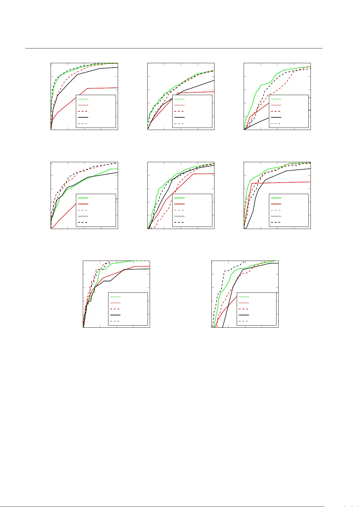
Leave a Comment