LUNAR: Cellular Automata for Drifting Data Streams

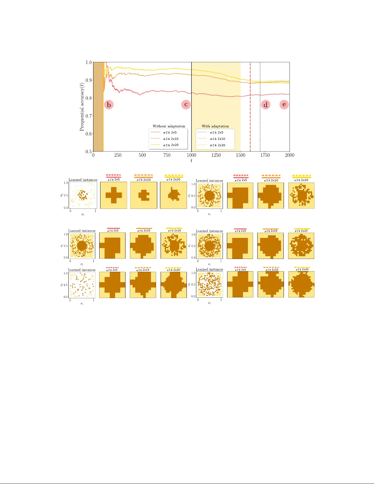
LUN AR: Cellular Automata for Drifting Data Streams Jesus L. Lobo a, ∗ , Javier Del Ser a,b,c , Francisco Herrera d a TECN ALIA, Basque Resear ch and T ec hnology Alliance (BRT A), 48160 Derio-Bizkaia, Spain b University of the Basque Country UPV/EHU , 48013 Bilbao, Spain c Basque Center for Applied Mathematics (BCAM), 48009 Bilbao, Spain d Andalusian Resear ch Institute in Data Science and Computational Intelligence (DaSCI), University of Granada, 18071 Gr anada, Spain Abstract W ith the adv ent of huges volumes of data produced in the form of fast streams, real- time machine learning has become a challenge of rele v ance emerging in a plethora of real-world applications. Processing such fast streams often demands high memory and processing resources. In addition, they can be af fected by non-stationary phenomena (concept drift), by which learning methods have to detect changes in the distrib ution of streaming data, and adapt to these e v olving conditions. A lack of efficient and scal- able solutions is particularly noted in real-time scenarios where computing resources are sev erely constrained, as it occurs in networks of small, numerous, interconnected processing units (such as the so-called Smart Dust, Utility Fog, or Swarm Robotics paradigms). In this work we propose LUNAR , a str eamified version of cellular au- tomata de vised to successfully meet the aforementioned requirements. It is able to act as a real incremental learner while adapting to drifting conditions. Extensi ve simula- tions with synthetic and real data will provide evidence of its competitive beha vior in terms of classification performance when compared to long-established and successful online learning methods. K eywor ds: Cellular automata, real-time analytics, data streams, concept drift 1. Introduction Real-T ime Analytics (R T A), also referred to as stream learning, acquired special rele v ance years ago with the advent of the Big Data era (Laney, 2001; Bifet, Gav ald ` a, Holmes & Pfahringer, 2018), becoming one of its most widely acknowledged chal- lenges. Data streams are the basis of the real-time analytics, composed by sequences of items, each having a timestamp and thus a temporal order , and arri ving one by one. Due to the incoming sheer volume of data, real-time algorithms cannot explicitly access all ∗ Corresponding author: jesus.lopez@tecnalia.com (Jesus L. Lobo). TECNALIA, E-700, 48160 De- rio (Bizkaia), Spain. Tl: +34 946 430 50. Fax: +34 901 760 009. Pr eprint submitted to Elsevier F ebruary 7, 2020 historical data because the storage capacity needed for this purpose becomes unman- ageable. Indeed, data streams are fast and large (potentially , infinite), so information must be extracted from them in real-time. Under these circumstances, the consumption of limited resources (e.g. time and memory) often implies sacrificing performance for ef ficiency of the learning technique in use. Moreov er , data streams are often produced by non-stationary phenomena, which imprint changes on the distribution of the data, leading to the emergence of the so-called concept drift . Such a drift causes that pre- dicti ve models trained over data flo ws become ev entually obsolete, and do not adapt suitably to new distributions. Therefore, these predictiv e models need to be adapted to these changes as fast as possible while maintaining good performance scores (Gama, ˇ Zliobait ˙ e, Bifet, Pechenizkiy & Bouchachia, 2014). For all these reasons, the research community has dev oted intense ef forts tow ards the dev elopment of Online Learning Methods (OLMs) capable of efficiently undertak- ing predictiv e tasks over data streams under minimum time and memory requirements (W idmer & Kubat, 1996; Ditzler, Rov eri, Alippi & Polikar, 2015; W ebb, Hyde, Cao, Nguyen & Petitjean, 2016; Lu, Liu, Dong, Gu, Gama & Zhang, 2018; Losing, Hammer & W ersing, 2018; Lobo, Del Ser , Bifet & Kasabo v, 2020). The need for ov ercom- ing these setbacks stems from many real applications, such as sensor data, telecom- munications, social media, marketing, health care, epidemics, disasters, computer se- curity , electricity demand prediction, among many others ( ˇ Zliobait ˙ e, Pechenizkiy & Gama, 2016). The Internet of Things (IoT) paradigm deserves special attention at this point (Manyika, Chui, Bisson, W oetzel, Dobbs, Bughin & Aharon, 2015; De Fran- cisci Morales, Bifet, Khan, Gama & Fan, 2016), where a huge quantity of data is continuously generated in real-time by sensors and actuators connected by networks to computing systems. Man y of these OLMs are based on traditional learning meth- ods (i.e. Naiv e Bayes, Support V ector Machines, Decision T rees, Gaussian methods, or Neural Networks (Bifet, Gav ald ` a, Holmes & Pfahringer, 2018)), which hav e been str eamified to make them w ork incrementally and fast. By contrast, other models are al- ready suitable for mining data streams by design (Cervantes, Gagn ´ e, Isasi & Parizeau, 2018). Unfortunately , most existing RtML models show a high complexity and de- pendence on the value of their parameters, thereby requiring a costly tuning process (Losing, Hammer & W ersing, 2018). In addition, some of them are neither tractable nor interpretable, which are features lately targeted with particularly interest under the eXplainable Artificial Intelligence (XAI) paradigm (Barredo Arrieta, D ´ ıaz-Rodrguez, Del Ser , Bennetot, T abik, Barbado, Garc ´ ıa, Gil-L ´ opez, Molina, Benjamins, Chatila & Herrera, 2019). Nowadays, learning algorithms featuring these characteristics are still under acti ve search, calling for ne w approaches that blow a fresh breeze of nov elty ov er the field (Gama, ˇ Zliobait ˙ e, Bifet, Pechenizkiy & Bouchachia, 2014; Khamassi, Sayed-Mouchaweh, Hammami & Gh ´ edira, 2018). Cellular Automata (CA) become fashionable with the Conway’ s Game of Life in 1970, but scientifically rele v ant after the Stephen W olfram’ s study in 2002 (W olfram, 2002). Despite they are not widely used in data mining tasks, the Fa wcett’ s work (Fa wcett, 2008) showed how they can turn into a simple and lo w-bias data mining 2 method, robust to noise, and with competitiv e classification performances in many cases. Until no w , their appearance on the R T A has been timid, without providing e vi- dences of their capacity for incremental learning and drift adaptation. This work enters this research av enue by proposing the use of Cellular Automata for R T A. Our approach, hereafter coined as celluLar aUtomata for driftiNg dAta stReams ( LUNAR ), capitalizes on the acknowledged capacity of CA to model complex systems from simple structures. W e sho w the intersection of CA and R T A in the presence of concept drift, sho wing that CA are promising incremental learners capable of adapting to ev olving en vironments. Specifically , we provide a method to transform a traditional CA into its str eamified version ( sCA ) so as to learn incrementally from data streams. W e sho w that LUNAR performs competitiv ely with respect to other online learners on se veral real-world datasets. More precisely , we will provide informed answers to the follo wing research questions: • RQ1 : Does sCA act as a real incremental learner? • RQ2 : Can sCA ef ficiently adapt to ev olving conditions? • RQ3 : Does our LUNAR algorithm perform competitiv ely with respect to other con- solidated R T A approaches reported in the literature? The rest of the manuscript is organized as follo ws: first, Section 2 provides a general introduction to CA, placing an emphasis on their historical role in the pattern recogni- tion field, and concretely their relev ance for stream learning. Next, Section 3 delves into the methods and the LUNAR approach proposed in this work. Section 4 introduces the experimental setup, whereas Section 5 presents and discusses the obtained results from such experiments. Finally , Section 6 draws conclusions and future research lines related to this work. 2. Related W ork Before going into the technical details of the proposed approach, we herein provide a historical overvie w of CA (Subsection 2.1 ), along with a perspectiv e on how these models have been progressively adopted for pattern recognition (Subsection 2.3 ) and, more lately , stream learning (Subsection 2.4 ). 2.1. The Limelight Shone Down on Cellular Automata The journey of CA was initiated by John von Neumann (Neumann, Burks et al., 1966) and Ulam for the modeling of biological self-reproduction. They became really fashionable due to the popularity of Conway’ s Game of Life introduced by Gardner (Games, 1970) in the field of artificial life (Langton, 1986). Arguably , the most scien- tifically significant and elaborated work on the study of CA arriv ed in 2002 with the thoughtful studies of Stephen W olfram (W olfram, 2002). In recent years, the notion of complex systems prov ed to be a very useful concept to define, describe, and study 3 v arious natural phenomena observed in a v ast number of scientific disciplines. De- spite their simplicity , they are able to describe and reproduce many complex phenom- ena (W olfram, 1984) that are closely related to processes such as self-organization and emergence, often observed within se veral scientific disciplines: biology , chemistry and physics, image processing and generation, cryptography , ne w computing hardw are and algorithms designs (i.e., automata networks (Goles & Mart ´ ınez, 2013) or decon volution algorithms (Zenil, Kiani, Zea & T egn ´ er, 2019)), among many others (Ganguly , Sikdar , Deutsch, Canright & Chaudhuri, 2003; Bhattacharjee, Naskar , Roy & Das, 2016). CA hav e also been satisfactorily implemented for heuristics (Nebro, Durillo, Luna, Dor- ronsoro & Alba, 2009) and job scheduling (Xhafa, Alba, Dorronsoro, Duran & Abra- ham, 2008). Besides, the capability to perform universal computation (Cook, 2004) has been one of the most celebrated features of CA that has garnered the attention of the research community: an arbitrary T uring machine can be simulated by a cellular automaton, so uni versal computation is possible (W olfram, 2002). Considering their parallel nature (which allo ws special-purposed hardware to be implemented), CA are also called to be a breakthrough in paradigms such as Smart Dust (W arneke, Last, Liebowitz & Pister, 2001; Ilyas & Mahgoub, 2018), Utility Fog (Hall, 1996; Dastjerdi & Buyya, 2016), Microelectromechanical Systems (MEMS or “motes”) (Judy, 2001), or Swarm Intelligence and Robotics (Ramos & Abraham, 2003; Del Ser , Osaba, Molina, Y ang, Salcedo-Sanz, Camacho, Das, Suganthan, Coello & Herrera, 2019), due to their capability to be computationally complete. Microscopic sensors are set to re volutionize a range of sectors, such as space missions (Niccolai, Bassetto, Quarta & Mengali, 2019). The sensing, control, and learning algorithms that need to be embarked in such miniaturized devices can currently only be run on relati vely heavy hardware, and need to be refined. Howe ver , nature has shown us that this is possible in the brains of insects with only a fe w hundred neurons. CA can also be decisiv e in other paradigms such as Nanotechnology , Ubiquitous Computing (L ´ opez-de Ipi ˜ na, Chen, Mitton & Pan, 2017), and Quantum Computation (introduced by Feynman (Fe ynman, 1986)), particularly the Quantum CA (Lent, T ougaw , Porod & Bernstein, 1993; W atrous, 1995; Adamatzk y, 2018). Due to the miniaturization hurdles of these devices, CA for stream learning may become of interest when there is no enough capacity to store huges v olumes of data, and the computational capacity is very limited. After all, it is therefore not surprising that CA hav e receiv ed particular attention since the early days of CA in vestigation, and that CA for stream learning allows us to mov e in the correct direction in these scenarios, which are not far off the near future (Jaf feris, Helbling, Karpelson & W ood, 2019). 2.2. F oundations of Cellular Automata CA are usually described as discrete dynamical systems which present a universal computability capacity (W olfram, 2018). Their beauty lies in its simple local interac- tion and computation of cells, which results in a huge complex behavior when these cells act together . W e can find four mutually interdependent parts in CA: i) the lattice, ii) its states, 4 iii) the neighborhood, and i v) the local rules. A lattice is created by a grid of elements (cells), which can be composed in one, two or higher dimensional space, but typically composed of uniform squared cells in two dimensions. CA contain a finite set of dis- crete states , whose number and range are dictated by the phenomenon under study . W e find the simplest CA built using only one Boolean state in one dimension. The neighborhood , which is used to ev aluate a local rule , is defined by a set of neighbor- ing (adjacent) cells. A neighboring cell is any cell within a certain radius of the cell in question. Additionally , it is important to specify whether the radius R applies only along the axes of the cell space (von Neumann neighborhood), or if it can be applied diagonally (Moore neighborhood). In two dimensions, the R = 1 von Neumann neigh- borhood or the R = 1 Moore neighborhood are often selected (see Figure 1a ). Finally , a local rule defines the ev olution of each CA; it is usually realized by taking all states from all cells within the neighborhood, and by ev aluating a set of logical or arithmeti- cal operations written in the form of an algorithm (see Figure 1b ). W e can formally define a cellular automaton as follows, by adopting the notation used in (Kari, 2005): A ≐ ( d, S , f ⊞ , f ÿ ) , where d represents the dimension, S a finite set of discrete states, f ⊞ ( ⋅ ) is a function that giv en a cell’ s coordinates at its input, returns the neighbors of the cell to be used in the update rule, and f ÿ ( ⋅ ) is a function that updates the state of the cell at hand as per the states of its neighboring cells. Therefore, in the case of a radius R = 1 von Neumann neighborhood defined over a d = 2 -dimensional lattice, the set of neighboring cells and state of cell with coordinates c = [ i, j ] is gi ven by: f ⊞ ([ i, j ]) = {[ i, j + 1 ] , [ i − 1 , j ] , [ i, j − 1 ] , [ i + 1 , j ]} , (1) S ( c ) = S ([ i, j ]) = f ÿ ( S ([ i, j + 1 ]) , S ([ i − 1 , j ]) , S ([ i, j − 1 ]) , S ([ i + 1 , j ])) , (2) i.e., the states vector S ([ i, j ]) of the [ i, j ] cell within the lattice is updated according to the local rule f ÿ ( ⋅ ) applied over its neighbors gi ven by f ⊞ ([ i, j ]) . In general, in a d -dimensional space, a cell’ s von Neumann neighborhood will contain 2 d cells, and a Moore neighborhood will contain 3 d − 1 cells. W ith this in mind, a cellular automaton should e xhibit three properties to be treated as such: i) parallelism or synchr onicity (all of the updates to the cells compounding the lattice are done at once); ii) locality (when a cell [ i, j ] is updated, its state S [ i, j ] ) is based on the previous state of the cell and those of its nearest neighbors; and iii) homog eneity or pr operties-uniformity (the same update rule f ÿ ( ⋅ ) is applied to each cell). The use of CA for pattern recognition is not straightforward. Some modifications and considerations should be performed before using CA for pattern recognition, since we need to map a dataset to a cell space: • Grid of cells (lattice): despite being a natural fit to two-dimensional problems, CA must be extended to multiple dimensions to accommodate general pattern recognition tasks encompassing more dimensions. For n features, an approach adopted in the related literature is to assign one grid dimension to each feature of the dataset. Once dimensions of the grid hav e been set, we need to partition each grid dimension by the feature’ s values, obtaining an equal number of cells per dimension. T o do that, e venly spaced values based on the maximum and minimum feature values (with an 5 R 1 2 (a) ? ? (b) (c) 2x5 2x10 2x20 (d) Figure 1: V isual representation of CA for pattern recognition: (a) the von Neumann’ s (left) and Moore’ s (right) neighborhoods with radius R = 1 ; (b) the center cell examines its von Neumann’ s (left) and Moore’ s (right) neighborhoods and applies the local rule (majority vote) in a one-step update; (c) a tw o- dimensional dataset with instances X t = ( X 1 t , X 2 t ) falling between [ 2 , 6 ] (min/max X 1 t ) and [ − 2 , − 4 ] (min/max X 2 t ), and a grid divided into G = 2 bins; (d) von Neumann’ s automata ( R = 1 , d × G ) ability to learn the data distrib ution from a fe w instances, and running up to 7 iterations of the initialization step (generations). 6 additional mar gin ( mar g ) to ensure a minimal separation among feature’ s v alues) are used to create “bins” for each dimension of the data (see Figure 1c ), which ultimately yield the cells of the lattice. • States : a finite number of discrete states ∣ S ∣ are defined, corresponding to the number of classes considered in the task. • Local rule : in pattern recognition tasks the update rule f ( ⋅ ) can be set to very assorted forms, being the most straightforward a majority voting among the states (labels) of its neighbors, i.e. for d = 2 , S ([ i, j ]) = arg max s ∈ S  [ k,l ] ∈ f ⊞ ([ i,j ]) I ( S ([ k, l ]) = s ) , (3) where f ⊞ ([ i, j ]) returns the coordinates of neighboring cells of [ i, j ] , and I ( ⋅ ) is an auxiliary function taking value 1 if its argument is true (and 0 otherwise). Any other update rule can be defined to spread the state activ ation of each cell over its neighborhood (see Figure 1b ). • Neighborhood : it is necessary to specify a neighborhood and its radius. Although there are more types of local rules, “von Neumann” or “Moore” neighborhoods are often used (Figure 1a ). • Initialization : the grid is seeded depending on the feature v alues of the instances of the training dataset. Specifically , the state of each cell is assigned the label corre- sponding to the majority of training data instance with feature v alues falling within the range co vered by the cell. As a result, cells will or ganize themselv es into regions of similar labels (Figure 1d ). • Generations : after the initialization step, some cells can remain unassigned. Then, it is necessary to run the CA (generations) until no cells are left empty , and then continuing until either no changes are made or a fixed threshold is exceeded. Along this process, each cell computes its new state by applying the update rule ov er the cells in its immediate neighborhood. Each cell follows the same update rule, and all cells are updated simultaneously and synchronously . A critical characteristic of CA is that the update rule examines only its neighboring cells, so the processing is entirely local. No global or macro grid characteristics are computed whatsoev er (Figure 1d ). 2.3. Cellular Automata in P attern Recognition Despite the early findings presented in (Jen, 1986; Ragha v an, 1993; Chaudhuri, Cho wdhury , Nandi & Chattopadhyay, 1997), CA are not commonly used for pattern recognition. An exception is the work in (Fa wcett, 2008), where CA were used as a form of instance-based classifiers for pattern recognition. These kinds of classifiers are well known by the pattern recognition community in the form of instance-based learn- ing and nearest neighbors classifiers (Aha, Kibler & Albert, 1991; Duda, Hart & Stork, 7 2012). They represent regions of the instance space, so when a ne w instance needs to be classified, the y select one or more close neighbors in these regions, and use their labels to assign a label to the ne w instance. Ne vertheless, these are distinguished from CA in that they are not strictly local: there is no fixed neighborhood, hence an instance’ s nearest neighbor may change. In CA, by contrast, there is a fixed neighborhood, and the local interaction between cells influences the ev olution and behavior of each cell. Fa wcett, on the basis of Ultsch’ s work (Ultsch, 2002), put CA in value for the pattern recognition community by introducing them as a low-bias data mining method, simple but powerful for attaining massiv ely fine-grained parallelism, non-parametric, with an ef fecti ve and competiti ve classification performance in many cases (similar to that pro- duced by other complex data mining models), and robust to noise. Besides, they were found to perform well with relativ ely scarce data. All this prior evidence makes CA suited for pattern recognition tasks. Finally , it is worth highlighting the ability of CA to extract patterns from informa- tion and the possibility of generating tractable models, and being simple methods at the same time. This ability has encouraged the community to use them as a machine learn- ing technique. Concretely , their traceability and reversibility (Kari, 2018) are reno wned dri vers for their adoption in contexts where model explainability is sought (Ribeiro, Singh & Guestrin, 2016; Gunning, 2017; Barredo Arrieta, D ´ ıaz-Rodrguez, Del Ser , Bennetot, T abik, Barbado, Garc ´ ıa, Gil-L ´ opez, Molina, Benjamins, Chatila & Herrera, 2019). 2.4. Cellular Automata for Str eam Learning In a real-time data mining process (stream learning), data streams are read and pro- cessed once per arriving sample (instance). Algorithms learning from such streams (stream learners) must operate under a set of constrained conditions (Domingos & Hul- ten, 2003): • Each instance can be processed only once. • The processing time of each instance must be low . • Memory must be low as well, which implies that only a few instances of the stream should be explicitly stored. • The algorithm must be prepared for providing an answer (i.e. a prediction) at any time of the process. • Data streams e v olve along time, which is an aspect that should be mandatorily con- sidered. In mathematical terms, a stream learning process ev olving over time can be for- mally defined as follo ws: gi ven a time period [ 0 , t ] , we denote the historical set of instances as D 0 ,t = d 0 , . . . , d t , where d i = ( X i , y i ) is a data instance, X i is the fea- ture vector and y i its label. W e assume that D 0 ,t follo ws a certain joint probability 8 distribution P t ( X , y ) . Such data streams are usually af fected by non-stationary e vents (drifts) that ev entually change their distribution (concept drift), making predictiv e mod- els trained over these data obsolete. Bearing the previous notation in mind, concept drift at timestamp t + 1 occurs if P t ( X , y ) ≠ P t + 1 ( X , y ) , i.e. as a change of the joint probability distribution of X and y at time t . Since in stream learning we cannot explicitly store all past data to detect or quantify this change, concept drift detection and adaptation are acknowledged challenges for real-time processing algorithms (Lu, Liu, Dong, Gu, Gama & Zhang, 2018). T wo strategies are usually follo wed to deal with concept drift: • P assive , by which the model is continuously updated ev ery time new data instances are recei ved, ensuring a suf ficient le vel of div ersity in its captured knowledge to ac- commodate changes in their distribution; and • Active , in which the model gets updated only when a drift is detected. Both strategies can be successful in practice, howe ver , the reason for choosing one strategy ov er the other is typically specific to the application. In general, a passi ve strategy has shown to be quite ef fecti ve in prediction settings with gradual drifts and recurring concepts, while an acti ve strategy works quite well in settings where the drift is abrupt. Besides, a passive strategy is generally better suited for batch learn- ing, whereas an activ e strategy has been shown to work well in online settings (Gama, Medas, Castillo & Rodrigues, 2004; Bifet & Gav alda, 2007; Alippi, Boracchi & Rov eri, 2013). In this work we ha v e adopted an activ e strate gy due to the fact that stream learn- ing acts in an online manner . Stream learning under non-stationary conditions is a field plenty of ne w challenges that require more attention due to its impact on the reliability of real-world applica- tions. CA may provide a rev olutionary view on R T A. Unfortunately , as shown later in Section 2.2, the original form of CA for pattern recognition does not allo w for stream processing. A few timid attempts at incorporating CA concepts to R T A hav e been re- ported in the past. In (Hashemi, Y ang, Pourkashani & Kangav ari, 2007; Pourkashani & Kangav ari, 2008) a cellular automaton-based approach was used as a real-time in- stance selector for stream learning. The classification task is carried out in batch mode by other non-CA-based learning algorithms. This is an essential dif ference with re- spect to the LUNAR approach proposed in this work, as the CA approach in (Hashemi, Y ang, Pourkashani & Kanga v ari, 2007; Pourkashani & Kangav ari, 2008) is not used for the learning task itself, but rather as a complement to the learning algorithm under use. Besides, they do not answer the relev ant research questions posed in Section 1, which should be the basis for the use of CA in stream learning. The dev eloped LUNAR algorithm is a str eamified learning version of CA. It transforms CA into real incre- mental learners that incorporate an embedded mechanism for drift adaptation. In what follo ws we address the posed research questions by providing rationale on the design of LUNAR , and discussing on a set of experiments specifically dev oted to inform our answers. 9 3. Proposed A pproach: LUNAR As it has been pre viously mentioned, LUNAR relies on the usage of CA for R T A. In this section we first introduce the modifications to str eamify a CA pattern recognition approach (Subsection 3.1 ). Secondly , LUNAR is deeply detailed, grounded on the pre viously introduced material (Subsection 3.2 ). 3.1. Adapting Cellular Automata for Incr emental Learning The CA approach designed for pattern recognition can be adapted to cope with the constraints imposed by incremental learning. W e present the details of this adaptation, which we coin as str eamified Cellular Automaton ( sCA ), in Algorithm 1 (Streamified Cellular Automaton ( sCA )): • First, the sCA is created after setting the v alue of its parameters as per the dataset at hand (lines 1 to 5 ). • Then, a set of P preparatory data are used to initialize the grid off-line by assigning the states of the corresponding cells according to the instances’ v alues (lines 6 to 11 ). • After this preliminary process, it is important to note that sev eral preparatory data instances might collide into the same cell, thereby yielding sev eral state occurrences for that specific cell. Since each cell must possess only one state for prediction pur- poses, lines 12 to 16 aim at removing this multiplicity of states by assigning each cell the state that occurs most among the preparatory data instances that fell within its boundaries. • Similarly , we must ensure that all cells ha ve a state assigned, i.e. no empty grid cell status must be guaranteed. T o this end, lines 17 to 23 apply the local rule f ÿ ( ⋅ ) over the neighbors of ev ery cell, repeating the process (generations) until ev ery cell has been assigned a state. • This procedure can again render se v eral dif ferent states for a gi ven cell, so the pre vi- ously explained majority state assignment procedure is again enforced ov er all cells of the grid (lines 24 to 28 ). Once this preparatory process is finished, the sCA is ready for the test-then-train (Gama, ˇ Zliobait ˙ e, Bifet, Pechenizkiy & Bouchachia, 2014) process with the rest of the instances (lines 29 to 34 ). In this process, the sCA first predicts the label of the arriving instance (testing phase), and updates the limits to reconfigure the bins (training phase). By this way , the sCA always represents the currently pre v ailing distribution of the streaming data at its input. After that, the sCA updates the current state of the cell enclosing the instance with the true label of the incoming instance. As a result, the cells of sCA always ha ve an updated state according to the streaming data distrib ution. The details of the proposed LUNAR algorithm underline the main differences be- tween the CA v ersion for pattern recognition and sCA . W e highlight here the most rele v ant ones: 10 Algorithm 1: Str eamified Cellular Automaton ( sCA ) Input : Preparatory data instances [( X t , y t )] t = P − 1 t = 0 ; training/testing data for the rest of the stream [( X t , y t )] ∞ t = P ; the grid size G (bins per dimension); a local update rule f ÿ ( ⋅ ) ; a neighborhood function f ⊞ ( c ) for cell with coordinates c ∈ G = { 1 , . . . , G } d as its argument; a radius R for the neighborhood operator Output: T rained streamified CA ( sCA ), producing predictions  y t ∀ t ∈ [ P , ∞ ) 1 Let the number of dimensions d of the grid be the number of features in X t 2 Let the number of cell states ∣ S ∣ be the number of classes (alphabet of y t ) 3 Set an empty vector of state hits per e very cell: h c = [] ∀ c ∈ G 4 Initialize the limits of the grid: [( l im low n , l im hig h n )] d n = 1 5 Create the sCA grid as per G , n and [( l im low n , l im hig h n )] d n = 1 6 for t = 0 to P − 1 do // Preparatory process 7 Update limits as per X t , e.g., l im low n = min { l im low n , x n t } 8 Reconfigure grid bins as per G and the updated [( l im low n , l im hig h n )] d n = 1 9 Select the cell c in the grid that encloses X t 10 Append y t to the vector of state hits in the cell, e.g. h c ′ = [ h c ′ , y t ] 11 end 12 for c ∈ G do // Guaranteeing one state per cell 13 if ∣ h c ∣ > 1 then // More than 1 state hit in cell 14 S ( c ) = arg max s ∈ S ∑ ∣ h c ∣ i = 1 I ( h i c = s ) 15 end 16 end 17 while ∃ c ∈ G ∶ h c = [] do // Ensuring a hit in all cells 18 f or c ∈ G do 19 Compute the neighboring cells of c as per f ⊞ ( c ) and R 20 Compute state s ′ by applying rule f ÿ ( ⋅ ) ov er the neighboring cells 21 Append s ′ to h c , i.e., h c = [ h c , s ′ ] 22 end 23 end 24 for c ∈ G do // Guaranteeing one state per cell 25 if ∣ h c ∣ > 1 then // More than 1 state hit in cell 26 S ( c ) = arg max s ∈ S ∑ ∣ h c ∣ i = 1 I ( h i c = s ) 27 end 28 end 29 for t = P to ∞ do // Stream learning 30 Predict  y t as S ( c ) , with c denoting the coordinates of the cell enclosing X t 31 Update limits as per X t , e.g., l im low n = min { l im low n , x n t } 32 Reconfigure grid bins as per G and the updated [( l im low n , l im hig h n )] d n = 1 33 Update cell state to the verified class of the test instance: S ( c ) = y t 34 end 11 • Pr epar atory instances : a small portion of the data stream (preparatory instances [( X t , y t )] P − 1 t = 0 ) is used to perform the sCA initialization. Then, the grid is seeded with these data values, and sCA progresses through sev eral generations (and apply- ing the local rule) until all cells are assigned a state. W ith the traditional CA for pattern recognition, the whole dataset is a v ailable from the be ginning. Therefore, the CA initialization is not required. • An updated r epr esentation of the instance space : since historical data is not av ailable and data grow continuously , the sCA updates the cell bins of the grid every time a ne w data instance arriv es. By doing this, we ensure that the range of values of the instance space is updated during the streaming process. W ith the traditional CA for pattern recognition, as the whole training dataset is static, the grid boundaries and cell bins are calculated at the beginning of the data mining process, and remain unaltered during the test phase. • CA ’ s cells continuously updated : sCA ’ s cells are also updated when new data ar- ri ves by assigning the incoming label (state) to the corresponding cell. Instead of examining the cells in the immediate neighborhood of this corresponding cell during se veral generations (which would take time and computational resources), sCA just checks the previous state of the cell and the current state provided by the recent data instance. When both coincide, no change is required, but when they differ , the cell adopts the state of the incoming data instance. In this sense, sCA always represents the current data distribution. This is the way sCA works as an incremental learner . Ho we ver , with the traditional CA for pattern recognition, once initialized, a local rule is applied o ver successiv e generations to set the state of a giv en cell depending on the states of its neighbors. 3.2. LUNAR : a sCA with Drift Detection and Adaptation Abilities LUNAR blends together sCA and paired learning in order to cope with concept drift. In essence, a stable sCA is paired with a reactiv e one. The scheme inspires from the findings reported in (Bach & Maloof, 2008): a stable learner is incrementally trained and predicts considering all of its experience during the streaming process, whereas a reacti ve learner is trained and predicts based on its experience over a time window of length W . Any online learning algorithm can be used as a base learner for this strate gy . As shown in Algorithm 2 (Paired learning for OLMs), the stable learner is used for prediction, whereas the reacti ve learner is used to detect possible concept drifts: • While the concept remains unchanged, the stable learner pro vides a better perfor- mance than the reacti ve learner (lines 6 and 7 ). • A counter is arranged to count the number of times within the windo w that the reac- ti ve learner predicts correctly the stream data, and the stable learner produces a bad prediction (lines 8 to 10 ). 12 • If the proportion of these occurrences surpasses a threshold θ (line 11 ), a concept change is assumed to hav e occurred, the stable learner is replaced with the reactiv e one, and the stable learner is reinitialized. • Finally , both stable and reacti ve learners are trained incrementally (lines 15 and 16 ). Algorithm 2: Paired learning for OLMs Input : Preparatory data instances {( X t , y t )} t = P − 1 t = 0 ; training/testing data for the rest of the stream {( X t , y t )} ∞ t = P ; windo w size W for the reactive learner; threshold θ for substituting the stable learner with the reactiv e one; stream learning model f ( X ) Output: Updated stable and reactiv e learners f s ( ⋅ ) and f r ( ⋅ ) 1 Let c = [ c w ] W w = 1 be a circular list of W bits, each initially set to c w = 0 ∀ w 2 for t = 0 to P − 1 do // Preparatory process 3 T rain both f s ( ⋅ ) and f r ( ⋅ ) with ( X t , y t ) 4 end 5 for t = P to ∞ do // Stream learning 6 Let  y s = f s ( X t ) (output of the model) and  y r = f r ( X t ) 7 Set c 1 = 0 and c w = c w − 1 for w = 2 , . . . , W 8 if  y s ≠ y t and  y r = y t then 9 Set c 1 = 1 10 end 11 if W − 1 ∑ W w = 1 c w > θ then // Drift detection 12 Replace f s ( ⋅ ) with f r ( ⋅ ) (including its captured knowledge) 13 Set c w = 0 ∀ w = 1 , . . . , W 14 end 15 T rain f s ( ˙ ) incrementally with ( X t , y t ) 16 T rain f r ( ⋅ ) from scratch over {( X t ′ , y t ′ )} t t ′ = t − W + 1 17 end Algorithm 3 ( LUNAR ) describes in detail the proposed algorithm. In essence the ov erall scheme relies on a couple of paired sCA learners: one in charge of making predictions on instances arriving in the data stream ( stable sCA learner), whereas the other ( r eactive sCA learner) captures the most recent past knowledge in the stream (as reflected by a time window W ). As previously explained for generic paired learning, the comparison between the accuracies scored by both learners ov er the time windo w permits to declare the presence of a concept drift when the reactiv e learner starts pre- dicting more accurately than its stable counterpart. When this is the case, the grid state v alues of the reacti ve sCA is transferred to the stable automaton, and proceeds forward by predicting subsequent stream instances with an updated grid that potentially best represents the pre v ailing distrib ution of the stream. W e now summarize the most interesting capabilities of the LUNAR algorithm: • Incr emental learning : as it relies on sCA learners, LUNAR shows a natural ability to learn incrementally , which is a crucial requirement under the constrained conditions 13 Algorithm 3: LUNAR Input : Preparatory data instances {( X t , y t )} P − 1 t = 0 ; training/testing data for the rest of the stream ( X t , y t ) ∞ t = P ; windo w size W for the reactiv e sCA learner; threshold θ for substituting the stable sCA learner with the reacti ve one; sCA parameters G , f ÿ ( ⋅ ) , f ⊞ ( c ) and R as per Algorithm 1 Output: Updated stable and reacti ve learners sCA s and sCA r 1 Let c = [ c w ] W w = 1 be a circular list of W bits, each initially set to c w = 0 ∀ w 2 Perform lines 1 − 28 of Algorithm 1 for sCA s and sCA r ov er {( X t , y t )} P − 1 t = 0 3 for t = P to ∞ do // Stream learning 4 Let  y s = sCA s ( X t ) and  y r = sCA r ( X t ) as per line 30 of Algorithm 1 5 Set c 1 = 0 and c w = c w − 1 for w = 2 , . . . , W 6 if  y s ≠ y t and  y r = y t then 7 Set c 1 = 1 8 end 9 if W − 1 ∑ W w = 1 c w > θ then // Drift detection 10 Copy grid state v alues of sCA r to sCA s (kno wledge transfer) 11 Clear sCA r and seed it with {( X t ′ , y t ′ )} t t ′ = t − W + 1 12 Perform lines 1 − 28 of Algorithm 1 for sCA r 13 Set c w = 0 ∀ w = 1 , . . . , W 14 end 15 T rain sCA s incrementally with ( X t , y t ) // Lines 31 − 33 , Alg.1 16 T rain sCA r from scratch ov er {( X t ′ , y t ′ )} t t ′ = t − W + 1 17 end present in R T A. • F ew parameter s : LUNAR requires only a fe w parameters, a warmly welcome charac- teristic that simplifies the parameter tuning process in drifting en vironments. • Little data to be trained : LUNAR can learn a data distribution with relativ ely few instances which, in the context of stream learning, in volv es a quicker preparation (warm-up) phase. Howe ver , depending on the grid size G , se veral generations may be required to make all cells be assigned a state. This is exemplified in Figure 1d, which considers a dataset with 2 continuous features X t = ( X 1 t , X 2 t ) ∈ R [ 0 , 1 ] , and a binary target class y t ∈ { 0 , 1 } . Here, a d × G = 2 × 5 cellular automaton only needs 2 iterations of the loops in lines 12 to 28 (hereafter referred to as generation ) until all cells are assigned one and only one state (see Algorithm 1 ). Howe ver , the grid is coarse, and its distribution of states does not represent the distribution of the data stream. W ith a d × G = 2 × 10 cellular automaton, 4 generations are needed until no cells are left empty , and the representation of the data distribution is more finely grained. Finally , the d × G = 2 × 20 cellular automaton needs 7 generations until 14 no cells are left empty , yet the representation of the data distrib ution is well defined. A good balance between representati veness and complexity must be met in practice when deploying LUNAR in real setups. • Constrained scenarios : in setups where computational costs must be reduced ev en more, a subsampling strate gy is often recommended, where only a fraction of in- stances of the data stream is considered for model updating. In these scenarios, the capability of CA to represent the data distrib ution with a fe w instances fits perfectly . So does LUNAR by embracing sCA at its core. • Str eam learning under verification latency : learning in an en vironment where labels do not become immediately av ailable for model updating is known as verification la- tency . This requires mechanisms and techniques to propagate class information for- ward through se veral time steps of unlabeled data. This remains as an open challenge in the stream learning community (Krempl, ˇ Zliobaite, Brzezi ´ nski, H ¨ ullermeier , Last, Lemaire, Noack, Shaker , Sie vi, Spiliopoulou & Stefanowski, 2014). Here, LUNAR finds its gap as well, due to its capability of e volving through se veral generations and represents a data distribution from a fe w annotated data instances. • Evolving scenarios : by harnessing the concept of paired learners, LUNAR adapts to e v olving conditions where changes (drifts) prov oke that learning algorithms ha ve to forget and learn the old and the ne w concept, respectiv ely . • T ractable and interpr etable : both characteristics lately targeted with particularly in- terest under the eXplainable Artificial Intelligence (XAI) paradigm (Barredo Arrieta, D ´ ıaz-Rodrguez, Del Ser , Bennetot, T abik, Barbado, Garc ´ ıa, Gil-L ´ opez, Molina, Ben- jamins, Chatila & Herrera, 2019). Finally , LUNAR enters the stream learning scene as a new base learner for the state- of-the-art. 4. Experimental Setup W e hav e designed two experiments in order to answer the three research questions posed in the Section 1. The first experiment addresses the research questions RQ1 and RQ2 on the capability of sCA to learn incrementally and adapt to changes conditions, while the second experiment addresses RQ3 by discussing on the competitiv eness of our LUNAR algorithm with respect to other streaming learners. In all the experiments we hav e used the von Neumann neighborhood because it is linear in the number of dimensions of the instance space, so it scales well when dealing with problems of high dimensionality . In addition, this neighborhood is composed of less neighbors than in Moore’ s case, and the local rule is applied ov er less cells, which makes the process lighter and better for streaming scenarios in terms of computational and processing time costs. Regarding the performance measurement, we hav e adopted 15 the so-called pr equential accuracy (Dawid, V o vk et al., 1999) for all experiments, as it is a suitable metric to ev aluate the learner performance in the presence of concept drift (Dawid, V o vk et al., 1999; Gama, Sebasti ˜ ao & Rodrigues, 2013; Gama, ˇ Zliobait ˙ e, Bifet, Pechenizkiy & Bouchachia, 2014). This metric quantifies the av erage accuracy obtained by the prediction of each test instance before its learning in an online test- then-train f ashion, and is defined as: pr eAC C ( t ) = ⎧ ⎪ ⎪ ⎪ ⎨ ⎪ ⎪ ⎪ ⎩ pr eAC C ex ( t ) , if t = t ref , pr eAC C ex ( t - 1 ) + pr eAC C ex ( t ) − pr eAC C ex ( t - 1 ) t − t ref + 1 , otherwise, (4) where pr eAC C ex ( t ) = 0 if the prediction of the test instance at time t before its learning is wrong and 1 if it is correct; and t ref is a reference time that fixes the first time step used in the calculation. This reference time allo ws isolating the computation of the prequential accuracy before and after a drift has started. As for the initialization of sCA , follo wing Algorithm 1 we have used a reduced group of P preparatory instances. In the second experiment we have also used these instances to carry out the hyper -parameter tuning of the OLMs under analysis. The selection of the size of this preparatory data usually depends on the av ailable memory or the processing time we can take to collect or process these data. Finally , follo wing the recommendations of (Fa wcett, 2008), we ha ve assigned one grid dimension to each attribute. 4.1. F irst Experiment: Addressing RQ1 and RQ2 with sCA In order to address RQ1 and RQ2 , we ha ve used sev eral two-dimensional synthetic datasets for the first experiment, where results can be easily visualised and interpreted. Synthetic data are advisable because in real datasets is not possible to kno w exactly when a drift appears, which type of drift emerges, or ev en if there is any confirmed drift. Thus, it is not possible to analyze the beha vior of sCA in the presence of concept drift by only relying on real-world datasets. This being said, for this experiment we hav e used the sCA detailed in Section 3.1 (Algorithm 1 ). W e hav e compared its nai ve version with the one using an acti ve adap- tation mechanism: assuming a perfect drift detection (the drift point is known before- hand), once a drift occurs the grid of the sCA model is seeded with a W -sized window of past instances, which allo ws representing the current concept (data distribution). Then, sCA progresses again through sev eral generations (and applying the local rule) until all cells are assigned a state. As highlighted before, this ability of CA to represent a data distrib ution from a few instances is very valuable here, where only a limited slid- ing window is used to initialize the sCA grid. This experiment is designed to illustrate and visualize the operation of sCA in two dimensions (two features). W e use the renowned set of four balanced synthetic datasets ( CIRCLE , LINE , SINEH , and SINEV ) described in (Minku, White & Y ao, 2009). V ery briefly , these datasets contain one simulated drift characterized by low and high speed, resulting 2 dif ferent types of drift for each dataset. Speed is the in verse of the time taken for a 16 ne w concept to completely replace the pre vious one. Each dataset has 2 , 000 instances ( t ∈ { 1 , . . . , 2 , 000 } ), 2 normalized ( [ 0 , 1 ] ) continuous features X t = ( X 1 t , X 2 t ) , and a binary target class y t ∈ { 0 , 1 } . Drift occurs at t = 1 , 000 (where it goes from the old con- cept to the new one), and the drifting period is 1 for abrupt drifts (high speed datasets) and 500 for gradual ones (low speed datasets). For abrupt drifts we hav e opted for a small windo w size of W = 25 , whereas for gradual drifts we need a bigger window of W = 100 (Gama, Sebasti ˜ ao & Rodrigues, 2013). The size of this windo w will depend on the type of drift: a small window can assure fast adaptability in abrupt changes, while a large windo w produces lower variance estimators in stable phases, but cannot react quickly to gradual changes. Thus, sliding windo ws is a very common form of the so-called for getting mechanism (Gama, 2010), where outdated data is discarded and adapt to the most recent state of the nature, then emphasis is placed on error calculation from the most recent data instances. 4.2. Second Experiment: Addr essing RQ3 with LUNAR For the second experiment we hav e resorted to real-world datasets to confirm the competiti ve performance of LUNAR in a comparison with recognized OLMs in the lit- erature, answering RQ3 . In this case, since we deal with problems ha ving n features, an extensi ve use is to assign one grid dimension of the CA to each feature of the dataset. In this experiment, LUNAR is compared with paired learning models (see Algorithm 2 ) using at their core different online learning algorithms from the literature. These comparison counterparts ha ve been selected ov er others due to the fact that they are well-established methods in the stream learning community . Also because their imple- mentations are reliable and easily accessible in well-known Python frameworks such as scikit-multiflo w (Montiel, Read, Bifet & Abdessalem, 2018) and scikit-learn (Pe- dregosa, V aroquaux, Gramfort, Michel, Thirion, Grisel, Blondel, Prettenhofer , W eiss, Dubourg et al., 2011). As this is the first experiment carried out to kno w about their per- formance as incremental learners with drift adaptation, we hav e selected these reputed methods: • Stochastic Gradient Descent Classifier ( SGDC ) (Bottou, 2010) implements an stochas- tic gradient descent learning algorithm which supports different loss functions and penalties for classification. • Hoeffding T r ee ( HTC ) (Domingos & Hulten, 2000), also known as V ery Fast Decision T ree (VFDT), is an incremental an ytime decision tree induction algorithm capable of learning from massiv e data streams, assuming that the distribution of data instances does not change over time, and exploiting the fact that a small instance can often be enough to choose an optimal splitting attribute. • P assive Agr essive Classifier ( PAC ) (Crammer , Dekel, K eshet, Shalev-Shwartz & Singer, 2006) focuses on the target v ariable of linear regression functions, ˆ y t = ω T t ⋅ X t , where ω t is the incrementally learned weight vector . After a prediction is made, the algorithm receiv es the true target v alue y t and an instantaneous ε -insensiti ve hinge 17 loss function is computed to update the weight v ector . This loss function w as specif- ically designed to work with stream data, and is analogous to a standard hinge loss. The role of ε is to allow for a lower tolerance of prediction errors. Then, when a round finalizes, the algorithm uses ω t and the instance ( X t , y t ) to produce a new weight vector ω t + 1 , which is then used to predict the next incoming instance. • k-Near est Neighbours ( KNN ) (Read, Bifet, Pfahringer & Holmes, 2012), a well- kno wn lazy learner where the output is gi ven by the labels of the K training instances closest (under a certain distance measure) to the query instance X t . In its str eami- fied version, it works by keeping track of a sliding windo w of past training instances. Whene ver a query request is ex ecuted, the algorithm will search over its stored in- stances and find the K ≤ W closest neighbors in the window , again as per the selected distance metric. Three real-world datasets ha ve been utilized in this second experiment: • The Australian Ne w South W ales Electricity Market dataset ( ELEC2 ) (Gama, Medas, Castillo & Rodrigues, 2004) is a widely adopted real-world dataset in studies related to stream processing/mining, particularly in those focused on non-stationary settings. In essence the dataset represents electricity prices over time, which are not fixed and become affected by the demand and supply dynamics. It contains 45 , 312 instances dated from 7 May 1996 to 5 December 1998 . Each instance X t of the dataset refers to a period of 30 minutes, and has d = 5 features (day of week, time stamp, NSW elec- tricity demand, V ic electricity demand, and scheduled electricity transfer between states). The target variable y t to be predicted is binary , and identifies the change of the price related to a moving a verage of the last 24 hours. The class le vel only reflect de viations of the price on a one day a verage, and removes the impact of longer term price trends. • The Gi ve Me Some Credit dataset ( GMSC 1 ) correspond to a credit scoring task in which the goal is to decide whether a loan should be granted or not (binary target y t ). This is a core decision for banks due to the risk of unexpected expenses and fu- ture la wsuits. The dataset comprises supervised historical data of 150 , 000 borrowers described by d = 10 features. • The POKER-HAND dataset 2 originally consists of 1 , 000 , 000 stream instances. Each record is an example of a hand consisting of fi ve playing cards drawn from a standard deck of 52 cards. Each card is described by 2 attributes (suit and rank), giving rise to a total of d = 10 predicti v e attributes for ev ery stream instance X t . The goal is 1 A v ailable at: https://www.kaggle.com/c/GiveMeSomeCredit . Last accessed on De- cember 5th, 2019. 2 A v ailable at: https://archive.ics.uci.edu/ml/datasets/Poker+Hand . Last ac- cessed on December 5th, 2019. 18 to predict the poker hand upon such features, out of a set of ∣ S ∣ = 10 possible poker hands (i.e., multiclass classification task). In order to alleviate the computational effort needed to run the entire benchmark, we have selected 20 , 000 instances of each dataset. W e hav e considered the first 50% of the datasets ( 10 , 000 instances) to tune the parameters of the OLMs and to seed LUNAR , whereas the rest 50% has been used for prediction and performance assessment. Each experiment has been carried out 25 times in the case of SGDC , PAC and KNNC to ac- count for the stochasticity of the hyperparameter search algorithm and their learning procedure. Indeed, the considered online models are sensible to parameter values. Thus we hav e performed a randomized hyper -parameter tuning ov er preparatory in- stances, obtaining different hyper parameter settings for each run. T able 1 summarizes the parameters that ha ve participated in each randomized search process, follo wing the nomenclature of the scikit-learn 3 and scikit-multiflo w 4 frame works. In the case of HTC , we found experimentally that its default values (see documentation of scikit-multiflow for more details) ha ve work ed very well in all datasets, so it was not necessary to carry out the randomized search on hyper parameters, which helped speed up the e xperimen- tation. Finally , the same window size W than LUNAR has been assigned to KNNC for the sake of a fair comparison between them. Model Parameters V alues used T uning SGDC alpha 10 − x , x ∈ { − 1 , − 2 , . . . , − 6 } yes loss ‘perceptron’, ‘hinge’, ‘log’, ‘modified huber’, ‘squared hinge’ learning rate ‘constant’, ‘optimal’, ‘in vscaling’, ‘adapti ve’ eta0 0 . 1 , 0 . 5 , 1 . 0 penalty None, ‘l2’, ‘l1’, ‘elasticnet’ max iter 1 , 100 , 200 , 500 PAC C 0 . 001 , 0 . 005 , 0 . 01 , 0 . 05 , 0 . 1 , 0 . 5 , 1 . 0 yes max iter 1 , 100 , 200 , 500 KNNC n neighbors 5 , 10 , 15 , 25 , 50 yes leaf size 5 , 10 , 20 , 30 algorithm ‘auto’ weights ‘uniform’, ‘distance’ HTC grace period 200 no split criterion ‘info gain’ leaf pr ediction ‘nba’ nb thr eshold 0 T able 1: Parameters that hav e participated in each randomized searching process of SGDC , PAC and KNNC . In the case of HTC its default values show a good enough performance and has not participated in the randomized hyperparameter searching process. This has alleviated the computing cost of the experiments. Finally , T able 2 summarizes the parameter settings of LUNAR and the OLMs used for the real-world e xperiments. 3 https://scikit-learn.org/. Last access in December 5th, 2019. 4 https://scikit-multiflow .github .io/. Last access in December 5th, 2019. 19 Model Parameter Real data Synthetic data ELEC2 GMSC POKER-HAND All models P 50% of the considered stream length 5% of the considered stream length W 50 instances 250 instances 250 instances 25 , 50 , 100 instances LUNAR f ⊞ ( ⋅ ) von Neumann f ÿ ( ⋅ ) Majority voting from Expression (3) R 1 ( ( ) S { 0 , 1 } { 0 , 1 } { 0 , 1 , . . . , 9 } { 0 , 1 } d × G 5 × 5 10 × 3 10 × 3 2 × 5 , 2 × 10 , 2 × 20 θ 0 . 0 5 0 . 01 0 . 001 Not applicable SGDC 0 . 8 0 . 001 0 . 1 HTC 0 . 1 0 . 0001 0 . 01 PAC θ 0 . 8 0 . 001 0 . 1 Not used KNNC 0 . 1 0 . 001 0 . 001 T able 2: Parameters configuration for LUNARand the considered OLMs in synthetic ( RQ1 and RQ2 ) and real-world experiments ( RQ3 ). 5. Results and Analysis Next, we present the results for the two experiments, organizing the fore going anal- ysis and discussion in terms of the research questions posed in Section 1: 5.1. RQ1 : Does sCA act as a r eal incr emental learner? Definitely yes. If we combining the definition of incremental learning suggested by (Giraud-Carrier, 2000; Lange & Zilles, 2003) with Kunche v a’ s and Bifet’ s desiderata for non-stationary learning (Kunche va, 2004; Bifet, Gav ald ` a, Holmes & Pfahringer, 2018), incremental learning can be understood as the capacity to process and learn from data in an incremental fashion, and to deal with data changes (drifts) that may occur in the en vironment. Therefore, the properties that guide the creation of incremental learning algorithms (Ditzler & Polikar, 2012) are: • Learning new knowledge : this feature is essential for online learners that hav e to be deployed ov er non-stationary settings. T o pro vide evidence that SCA incorporates this characteristic, Figures 2 and 4 summarize the performance results obtained over two synthetic datasets ( CIRCLE and SINEH ) with an abrupt drift occurring at t = 1000 , and assuming to hav e been detected at t = 1025 . The adaptation mechanism resorts to a window of W = 25 past data instances; upon the detection of the drift, the entire knowledge contained in the cellular automata (i.e. the distribution of cell states) is erased, and the automata is seeded with the instances falling in the last W - sized window . Although the abrupt drift obliges to learn quickly the ne w concept and forgetting the old one, we observe in these plots that sCA excels at this task, yielding a prequential accuracy ov er time that does not get apparently af fected by the change of concept. • Pr eserving pr evious knowledge : related to the previous property , gradual drifts re- quire maintaining part of the previous concept over time, so that the ev olved model 20 le verages the retained knowledge during its transition to the new concept. This is clearly shown in Figures 3 and 5, which both focus on CIRCLE and SINEH respec- ti vely , sho wing a gradual drift at t = 1000 , and assuming a drift detection at t = 1600 . The adaptation mechanism resorts to a window of W = 100 past data instances. In particular , the prequential accuracy results and subplots therein included sho w that sCA can preserve the old concept while learning the ne w one through the implemen- tation of a forgetting strate gy . • One-pass (incremental) learning : through preceding sections we have elaborated on the incremental learning strate gy of sCA (lines 30 to 33 in Algorithm 1 ), by which it is able to learn one instance at a time without requiring any access to historical data. • Dealing with concept drift : Finally , we have seen in the previous experiments that sCA is capable of dealing with e v olving conditions by using a drift detection and by implementing an adaptation scheme. W e will later rev olve around these results. 21 2x5 2x10 2x20 2x5 2x10 2x20 (a) 2x5 2x10 2x20 (b) 2x5 2x10 2x20 (c) 2x5 2x10 2x20 2x5 2x10 2x20 (d) 2x5 2x10 2x20 2x5 2x10 2x20 (e) Figure 2: Learning and adaptation of von Neumann’ s sCA of different grid sizes for the CIRCLE dataset, which exhibits an abrupt drift at t = 1000 . The drift is detected at t = 1025 and then the adaptation mechanism, which uses a window of instances W = 25 , is triggered. (a) Performance comparison at points b (initial), c (just before the drift occurs), d ( W = 25 instances after drift detection and the adaptation mechanism were triggered), and e (final). The dashdotted line points out the drift detection and the dotted line the point in which the performance is measured. The shaded area corresponds to the preparatory instances. (b) The cells of sCA s are seeded with the preparatory instances ( b ). (c) The learning process of sCA before drift occurs ( c ). (d) The learning process of sCA after the drift occurs, and ho w those with the adaptation mechanism is initialized and seeded with a set of W = 25 past instances ( d ). (e) The learning process of sCA until the end of the stream ( e ). 22 2x5 2x10 2x20 2x5 2x10 2x20 (a) 2x5 2x10 2x20 (b) 2x5 2x10 2x20 (c) 2x5 2x10 2x20 2x5 2x10 2x20 (d) 2x5 2x10 2x20 2x5 2x10 2x20 (e) Figure 3: Learning and adaptation of von Neumann’ s sCA of different grid sizes for the CIRCLE dataset, which exhibits a gradual drift at t = 1000 . The drift is detected at t = 1600 , and then the adaptation mechanism, which uses a windo w of instances W = 100 , is triggered. The interpretation of the remaining plots is the same than those in Figure 2. 23 2x5 2x10 2x20 2x5 2x10 2x20 (a) 2x5 2x10 2x20 (b) 2x5 2x10 2x20 (c) 2x5 2x10 2x20 2x5 2x10 2x20 (d) 2x5 2x10 2x20 2x5 2x10 2x20 (e) Figure 4: Learning and adaptation of v on Neumann’ s sCA of dif ferent grid sizes for the SINEH dataset, which exhibits an abrupt drift at t = 1000 . The drift is detected at t = 1025 and then the adaptation mechanism, which uses a windo w of instances W = 25 , is triggered. The interpretation of the remaining plots is the same than those in Figure 2. 24 2x5 2x10 2x20 2x5 2x10 2x20 (a) 2x5 2x10 2x20 (b) 2x5 2x10 2x20 (c) 2x5 2x10 2x20 2x5 2x10 2x20 (d) 2x5 2x10 2x20 2x5 2x10 2x20 (e) Figure 5: Learning and adaptation of v on Neumann’ s sCA of dif ferent grid sizes for the SINEH dataset, which exhibits a gradual drift at t = 1000 . The drift is detected at t = 1600 and then the adaptation mechanism, which uses a windo w of instances W = 100 , is triggered. The interpretation of the remaining plots is the same than those in Figure 2. 25 5.2. RQ2 : Can sCA successfully adapt to evolving conditions? In a nutshell, the answer is yes. Ho we ver , the success rate depends on the type of drift and the size G of the CA grid. This is empirically sho wn in Figures 2 and 4 for abrupt drifts, where we hav e ap- plied an adaptation mechanism to a sCA of dif ferent grid sizes ov er the CIRCLE and SINEH datasets, respectively . Once the drift appears at t = 1000 (solid vertical line) and is detected (dashdotted vertical line), we observe that sCA with and without adaptation mechanism perform equal at points b and c . But when the adaptation mechanism is triggered we see at point d ( 25 instances after drift detection and adaptation) and e (the end of the data stream) that sCA using grids of d × G = 2 × 10 and d × G = 2 × 20 obtain better prequential accuracies when incorporating an adaptation mechanism. In the case of CIRCLE dataset, the adaptiv e versions of sCA obtain an av erage prequen- tial accuracy of 0 . 873 ( 2 × 10 ) and 0 . 900 ( 2 × 20 ) versus their non-adapti ve counterparts, which respecti vely score accuracies of 0 . 866 and 0 . 880 . The same situation holds with the SINEH dataset, where again adaptiv e sCA s obtain average prequential accuracies of 0 . 773 ( 2 × 10 ) and 0 . 833 ( 2 × 20 ) against their non-adaptiv e versions ( 0 . 765 and 0 . 808 , respecti vely). The adaptiv e versions are able to forget quickly the old concept because they are reinitialized with a fe w instances ( 25 ) of the new concept, as opposed to the non-adapti ve versions which keep the old concept along time (see Figures 2d and 4d ). At point e (Figures 2e and 4e ), we can observe some differences in the learning of both v ersions. In the case of the small grid size 2 × 5 , neither adaptiv e nor non-adaptiv e versions are able to learn the concepts properly and establishing the boundaries be- tween classes, yielding a poor classification performance. Therefore, when the change from the old to the new concept is abrupt, the fast for getting of the old concept be- comes primordial (Gama, Sebasti ˜ ao & Rodrigues, 2013). For a complete comparison with more datasets we refer to T able 3. No w , we focus on gradual drifts of CIRCLE and SINEH dataset (Figures 3 and 5 respecti vely), where a gradual drift also occurs at ( t = 1 , 000 ). Figures 3a and 5a, and T able 3, sho w how both sCA with and without adaptation mechanism obtain almost the same mean prequential accuracy . As the old concept disappears slowly while the ne w one also does it slowly , the adapti ve v ersion with a window of instances ( w = 100 ) and the non-adaptiv e version do preserve the old concept while learn the ne w one. Even so, we can observe slight improv ements of adapti ve versions over the non-adapti v e ones at points d and e . These dif ferences are bigger in the case of sCA with a 2 × 20 grid: 0 . 894 for the adaptiv e version against 0 . 888 for the non-adaptiv e version ( CIRCLE at point d ), 0 . 897 for the adapti ve version against 0 . 881 for the non-adaptiv e version ( CIRCLE at point e ), 0 . 812 for the adapti ve version against 0 . 811 for the non-adapti ve version ( SINEH at point d ), and 0 . 820 for the adapti ve version against 0 . 811 for the non-adaptiv e version ( SINEH at point e ). Again, in the case of a 2 × 5 grid, due to the small grid size neither adaptiv e nor non-adaptiv e versions are able to learn the concepts properly and establishing the boundaries between classes, achie ving a poor classification performance. For the case of sCA 2 × 10 , because the drift is gradual, the grid size does not allo w for capturing well enough the differences of both 26 concepts. Finally , when the change from the old concept to the ne w one is gradual, an slo w for getting of the old concept becomes primordial (Gama, Sebasti ˜ ao & Rodrigues, 2013). Synthetic datasets sCA d × G preACC ( t ) c d e A verage CIRCLE (abrupt) Adaptiv e 2 × 5 0 . 827 0 . 822 0 . 827 0 . 794 2 × 10 0 . 928 0 . 918 0 . 905 0 . 873 2 × 20 0 . 958 0 . 943 0 . 931 0 . 900 Non-adaptiv e 2 × 5 0 . 827 0 . 822 0 . 828 0 . 795 2 × 10 0 . 928 0 . 915 0 . 892 0 . 866 2 × 20 0 . 958 0 . 939 0 . 881 0 . 880 CIRCLE (gradual) Adaptiv e 2 × 5 0 . 827 0 . 816 0 . 820 0 . 789 2 × 10 0 . 928 0 . 885 0 . 890 0 . 867 2 × 20 0 . 958 0 . 894 0 . 897 0 . 890 Non-adaptiv e 2 × 5 0 . 827 0 . 817 0 . 820 0 . 789 2 × 10 0 . 928 0 . 886 0 . 891 0 . 868 2 × 20 0 . 958 0 . 888 0 . 881 0 . 888 LINE (abrupt) Adaptiv e 2 × 5 0 . 795 0 . 784 0 . 783 0 . 754 2 × 10 0 . 928 0 . 912 0 . 913 0 . 868 2 × 20 0 . 972 0 . 959 0 . 957 0 . 911 Non-adaptiv e 2 × 5 0 . 795 0 . 785 0 . 783 0 . 754 2 × 10 0 . 928 0 . 905 0 . 900 0 . 861 2 × 20 0 . 972 0 . 953 0 . 887 0 . 883 LINE (gradual) Adaptiv e 2 × 5 0 . 795 0 . 721 0 . 729 0 . 731 2 × 10 0 . 928 0 . 870 0 . 880 0 . 855 2 × 20 0 . 972 0 . 910 0 . 918 0 . 898 Non-adaptiv e 2 × 5 0 . 795 0 . 722 0 . 728 0 . 731 2 × 10 0 . 928 0 . 871 0 . 879 0 . 855 2 × 20 0 . 972 0 . 903 0 . 893 0 . 895 Synthetic datasets sCA d × G preACC ( t ) c d e A verage SINEV (abrupt) Adaptiv e 2 × 5 0 . 833 0 . 822 0 . 811 0 . 777 2 × 10 0 . 933 0 . 920 0 . 921 0 . 877 2 × 20 0 . 960 0 . 947 0 . 948 0 . 907 Non-adaptiv e 2 × 5 0 . 833 0 . 823 0 . 811 0 . 777 2 × 10 0 . 933 0 . 912 0 . 905 0 . 867 2 × 20 0 . 960 0 . 939 0 . 876 0 . 879 SINEV (gradual) Adaptiv e 2 × 5 0 . 833 0 . 753 0 . 756 0 . 757 2 × 10 0 . 933 0 . 881 0 . 891 0 . 866 2 × 20 0 . 960 0 . 893 0 . 906 0 . 893 Non-adaptiv e 2 × 5 0 . 833 0 . 754 0 . 757 0 . 757 2 × 10 0 . 933 0 . 882 0 . 892 0 . 867 2 × 20 0 . 960 0 . 884 0 . 879 0 . 890 SINEH (abrupt) Adaptiv e 2 × 5 0 . 514 0 . 514 0 . 501 0 . 473 2 × 10 0 . 822 0 . 811 0 . 806 0 . 773 2 × 20 0 . 889 0 . 874 0 . 877 0 . 833 Non-adaptiv e 2 × 5 0 . 514 0 . 514 0 . 503 0 . 474 2 × 10 0 . 822 0 . 804 0 . 790 0 . 765 2 × 20 0 . 889 0 . 862 0 . 822 0 . 808 SINEH (gradual) Adaptiv e 2 × 5 0 . 514 0 . 513 0 . 510 0 . 478 2 × 10 0 . 822 0 . 756 0 . 770 0 . 756 2 × 20 0 . 889 0 . 812 0 . 820 0 . 818 Non-adaptiv e 2 × 5 0 . 514 0 . 514 0 . 511 0 . 478 2 × 10 0 . 822 0 . 763 0 . 774 0 . 757 2 × 20 0 . 889 0 . 811 0 . 811 0 . 817 T able 3: Comparativ e results of sCA with and without adaptiv e mechanism with different grid sizes for synthetic CIRCLE , LINE , SINEV and SINEH datasets. The prequential accuracy is measured at points c (before the drift occurs), d (after drift occurs and adaptation mechanism has been triggered), and e (final). The last column amounts to the mean prequential accuracy av eraged over the duration of the whole stream. In light of the above claim, we can finally confirm that in case of abrupt drifts we should opt for small grid sizes G , which is better in terms of computational cost. Ho we ver , for gradual drifts the grid should be made finer in order to emphasize the dif ferences between adaptiv e and non-adaptiv e versions. For the sake of space, only the cases of CIRCLE and SINEH datasets are presented in Figures 2 (abrupt drift) and 3 (gradual drift), and 4 (abrupt drift) and 5 (gradual drift), respectiv ely . The results for all the synthetic datasets can be found in T able 3. 5.3. RQ3 : Is LUNAR competitive in comparison with other consolidated OLMs of the literatur e? In T able 4 and Figure 6 we analyze the competitiv eness of LUNAR in terms of clas- sification performance for the considered real-world datasets. In the ELEC2 dataset, only SGDC ( 0 . 820 ) outperforms LUNAR ( 0 . 763 ), and HTC shows almost the same score ( 0 . 766 ). In case of the GMSC dataset, only HTC ( 0 . 910 ) and PAC ( 0 . 891 ) outperforms LUNAR ( 0 . 869 ). For the POKER-HAND dataset, only HTC ( 0 . 573 ) and KNNC ( 0 . 567 ) outperforms LUNAR ( 0 . 527 ). 27 Follo wing the e v aluation method used in (Bifet, Holmes, Pfahringer & Frank, 2010), the column Global mean preACC of T able 4 av erages the results in all datasets, and sho ws how LUNAR ( 0 . 719 ) is the second best method, only surpassed by HTC ( 0 . 749 ), which is ar guably one of the best stream learners in the field. After the analysis of the results, we can confirm that effecti vely LUNAR has turned into a very competitiv e stream learning method. Method Dataset preA CC (mean ± std) Global mean preACC LUNAR ELEC2 0 . 763 ± 0 . 0 0.719 ± 0.0 GMSC 0 . 869 ± 0 . 0 POKER-HAND 0 . 527 ± 0 . 0 SGDC ELEC2 0 . 820 ± 0 . 058 0 . 703 ± 0 . 068 GMSC 0 . 845 ± 0 . 085 POKER-HAND 0 . 446 ± 0 . 061 HTC ELEC2 0 . 766 ± 0 . 0 0.749 ± 0.0 GMSC 0 . 910 ± 0 . 0 POKER-HAND 0 . 573 ± 0 . 0 PAC ELEC2 0 . 670 ± 0 . 043 0 . 685 ± 0 . 030 GMSC 0 . 891 ± 0 . 032 POKER-HAND 0 . 496 ± 0 . 015 KNNC ELEC2 0 . 621 ± 0 . 019 0 . 670 ± 0 . 029 GMSC 0 . 822 ± 0 . 014 POKER-HAND 0 . 567 ± 0 . 055 T able 4: Comparativ e results of LUNAR with other stream learners in real-world datasets. The column preA CC (mean ± std) denotes the mean prequential accuracy of every method in each dataset. The column Global mean preA CC presents the mean prequential accurac y for all datasets of each method, and serves as a reference for a global comparison. Global results of the two best methods are marked in bold. 5.4. F inal Observations, Remarks and Recommendations Once the three research questions hav e been thoroughly answered, it is worth dis- cussing some general recommendations related to LUNAR . When designing a sCA for non-stationary scenarios, we should consider that generally we will assign one grid dimension to each feature of the dataset, thus as many dimensions in the grid and as many cells per feature, as much computational cost and more processing time will be required. Specifically , provided that a problem with d dimensions is under target, and gi ven a granularity (size) of the grid giv en by G , the worst-case comple xity of predict- ing the class of a giv en test instance X t is giv en by O ( G d ) , which is the time taken by a single processing thread to explore all cells of the d -dimensional grid of cells and discriminate the cell enclosing X t . Due to the exponential comple xity , we recommend the use of sCA (and CA in pattern recognition in general) in datasets with a lo w num- 28 U (a) ELEC2 dataset U (b) GMSC dataset U (c) POKER-HAND dataset Figure 6: Prequential accuracy pr eAC C ( t ) for LUNAR and the OLMs under consideration in the se- lected real-world datasets. The first 50% of the dataset is for preparatory instances, while the rest is adopted as streaming test-then-train instances. A moving window of 500 instances has been applied in order to smooth out short-term fluctuations and to furnish a more friendly visualization. 29 ber of features. Nev ertheless, the search process ov er the grid’ s cells can be easily parallelized, hence allo wing for fast prediction and cell updating speeds. W e also pause at the str eamified version of the KNNC model, whose similarity to LUNAR calls for a brief comparison among them. In essence, both learning models rely on the concept of neighborhood in the feature space, induced by either the selected measure of similarity among instances ( KNNC ) or the arrangement of cells in a grid ( LUNAR ). W e ha ve seen in T able 4 that our proposed method overcomes the results of KNNC in ELEC2 and GMSC datasets. Here it is worth mentioning that in order to ha ve a fair comparison between both methods, the number of nearest neighbors to search for in the KNNC method has been properly optimized before the streaming process runs. Furthermore, the maximum size of the window storing the last viewed instances of KNNC has been set equal to the W parameter in LUNAR . The capability of the sCA grid’ s cells to reflect and maintain the prev ailing knowledge in the stream renders a superior performance than that of fered by the KNNC method when computing the similarity ov er the W -sized window of past instances. 6. Conclusions and Future W ork Cellular automata ha ve been successfully applied to different real-world applica- tions since their inception sev eral decades ago. Among them, pattern recognition has been proven to be a task in which the self-organization and modeling capabilities of cellular automata can yield significant performance gains. This work has b uilt upon this background to explore whether such benefits can also be extrapolated to real-time machine learning under non-stationary conditions, which is arguably among the hottest topics in Data Science now adays. Under the premises of real-time settings, aspects such as complexity and adaptability to changing tasks are also important modeling design dri vers that add to the performance of the model itself. The algorithm introduced in this work provides a new perspectiv e in the stream learning scene. W e hav e proposed a cellular automaton able to learn incrementally and capable of adapting to ev olving en vironments ( LUNAR ), sho wing a competitiv e classi- fication performance when is compared with other reputed state-of-the-art algorithms. LUNAR contributes to the discussion on ways to use cellular automata for paradigms in which the computation effort relies on a network of simple, interconnected devices with very lo w processing capabilities and constrained battery capacity (e.g. Utility Fog, Smart Dust, MEMS or Swarms). Under these circumstances, learning algorithms should be embarked in miniaturized devices running on low-po wer hardware with lim- ited storage. LUNAR has shown a well performance in practice over the datasets considered in this study , with empirical evidences of its adaptability when mining non-stationary data streams. Future work will be de voted towards experimenting with other local rules or neighborhoods to determine their ef fects on these identified properties of cellular au- tomata. Some preliminary experiments carried out off-line suggest that a sCA could also detect drifts, which, along with their simplicity , pav es the way towards adopting 30 them in activ e strategies for stream learning in non-stationary setups. W e ha ve also concei ved the possibility of configuring ensembles of sCA , wherein div ersity among the constituent automata can be induced by very di verse means (e.g. online bagging, boosting or probabilistic class switching). W e strongly belie ve that moving in this algorithmic direction may open up the chance of designing more po werful cellular au- tomata with complementary , potentially better capabilities to deal with stream learning scenarios. Acknowledgements This work has receiv ed funding support from the ECSEL Joint Undertaking (JU) under grant agreement No 783163 ( iDev40 project). The JU receiv es support from the European Union’ s Horizon 2020 research and innov ation programme, national grants from Austria, Belgium, Germany , Italy , Spain and Romania, as well as the European Structural and In vestment Funds. It has been also supported by the ELKAR TEK pro- gram of the Basque Government (Spain) through the VIRTUAL (ref. KK-2018/00096) research grant. Finally , Ja vier Del Ser has receiv ed funding support from the Con- solidated Research Group MATHMODE (IT1294-19), granted by the Department of Education of the Basque Gov ernment. References References Adamatzky , A. (2018). Cellular A utomata: A V olume in the Encyclopedia of Comple x- ity and Systems Science . Springer . Aha, D. W ., Kibler , D., & Albert, M. K. (1991). Instance-based learning algorithms. Machine learning , 6 , 37–66. Alippi, C., Boracchi, G., & Rov eri, M. (2013). Just-in-time classifiers for recurrent concepts. IEEE tr ansactions on neural networks and learning systems , 24 , 620–634. Bach, S. H., & Maloof, M. A. (2008). Paired learners for concept drift. In 2008 Eighth IEEE International Confer ence on Data Mining (pp. 23–32). IEEE. Barredo Arrieta, A., D ´ ıaz-Rodrguez, N., Del Ser , J., Bennetot, A., T abik, S., Barbado, A., Garc ´ ıa, S., Gil-L ´ opez, S., Molina, D., Benjamins, R., Chatila, R., & Herrera, F . (2019). Explainable artificial intelligence (xai): Concepts, taxonomies, opportunities and challenges to ward responsible ai. . Bhattacharjee, K., Naskar , N., Ro y , S., & Das, S. (2016). A surve y of cellular automata: types, dynamics, non-uniformity and applications. Natural Computing , (pp. 1–29). 31 Bifet, A., & Ga valda, R. (2007). Learning from time-changing data with adapti ve win- do wing. In Pr oceedings of the 2007 SIAM international confer ence on data mining (pp. 443–448). SIAM. Bifet, A., Ga v ald ` a, R., Holmes, G., & Pfahringer , B. (2018). Mac hine Learning for Data Streams with Practical Examples in MO A . MIT Press. https://moa.cms. waikato.ac.nz/book/ . Bifet, A., Holmes, G., Pfahringer , B., & Frank, E. (2010). Fast perceptron decision tree learning from ev olving data streams. In P acific-Asia conference on knowledge discovery and data mining (pp. 299–310). Springer . Bottou, L. (2010). Lar ge-scale machine learning with stochastic gradient descent. In Pr oceedings of COMPST A T’2010 (pp. 177–186). Springer . Cerv antes, A., Gagn ´ e, C., Isasi, P ., & Parizeau, M. (2018). Ev aluating and characteriz- ing incremental learning from non-stationary data. arXiv preprint , . Chaudhuri, P . P ., Chowdhury , D. R., Nandi, S., & Chattopadhyay , S. (1997). Additive cellular automata: theory and applications volume 1. John W iley & Sons. Cook, M. (2004). Uni versality in elementary cellular automata. Comple x systems , 15 , 1–40. Crammer , K., Dekel, O., K eshet, J., Shalev-Shw artz, S., & Singer , Y . (2006). Online passi ve-aggressi ve algorithms. Journal of Mac hine Learning Researc h , 7 , 551–585. Dastjerdi, A. V ., & Buyya, R. (2016). F og computing: Helping the internet of things realize its potential. Computer , 49 , 112–116. Dawid, A. P ., V ovk, V . G. et al. (1999). Prequential probability: Principles and proper- ties. Bernoulli , 5 , 125–162. De Francisci Morales, G., Bifet, A., Khan, L., Gama, J., & Fan, W . (2016). Iot big data stream mining. In Pr oceedings of the 22nd A CM SIGKDD International Confer ence on Knowledge Discovery and Data Mining (pp. 2119–2120). ACM. Del Ser , J., Osaba, E., Molina, D., Y ang, X.-S., Salcedo-Sanz, S., Camacho, D., Das, S., Suganthan, P . N., Coello, C. A. C., & Herrera, F . (2019). Bio-inspired computation: Where we stand and what’ s next. Swarm and Evolutionary Computation , 48 , 220– 250. Ditzler , G., & Polikar , R. (2012). Incremental learning of concept drift from streaming imbalanced data. IEEE transactions on knowledge and data engineering , 25 , 2283– 2301. 32 Ditzler , G., Roveri, M., Alippi, C., & Polikar , R. (2015). Learning in nonstationary en vironments: A surve y . IEEE Computational Intelligence Ma gazine , 10 , 12–25. Domingos, P ., & Hulten, G. (2000). Mining high-speed data streams. In Kdd (p. 4). volume 2. Domingos, P ., & Hulten, G. (2003). A general framework for mining massiv e data streams. Journal of Computational and Gr aphical Statistics , 12 , 945–949. Duda, R. O., Hart, P . E., & Stork, D. G. (2012). P attern classification . John W iley & Sons. Fa wcett, T . (2008). Data mining with cellular automata. ACM SIGKDD Explorations Newsletter , 10 , 32–39. Feynman, R. P . (1986). Quantum mechanical computers. F oundations of physics , 16 , 507–531. Gama, J. (2010). Knowledge discovery fr om data str eams . Chapman and Hall/CRC. Gama, J., Medas, P ., Castillo, G., & Rodrigues, P . (2004). Learning with drift detection. In Brazilian symposium on artificial intellig ence (pp. 286–295). Springer . Gama, J., Sebasti ˜ ao, R., & Rodrigues, P . P . (2013). On e v aluating stream learning algorithms. Machine learning , 90 , 317–346. Gama, J., ˇ Zliobait ˙ e, I., Bifet, A., Pechenizkiy , M., & Bouchachia, A. (2014). A survey on concept drift adaptation. ACM computing surve ys (CSUR) , 46 , 44. Games, M. (1970). The f antastic combinations of john conways new solitaire g ame life by martin gardner . Scientific American , 223 , 120–123. Ganguly , N., Sikdar , B. K., Deutsch, A., Canright, G., & Chaudhuri, P . P . (2003). A surve y on cellular automata, . Giraud-Carrier , C. (2000). A note on the utility of incremental learning. Ai Communi- cations , 13 , 215–223. Goles, E., & Mart ´ ınez, S. (2013). Neural and automata networks: dynamical behavior and applications volume 58. Springer Science & Business Media. Gunning, D. (2017). Explainable artificial intelligence (xai). Defense Advanced Re- sear ch Pr ojects Agency (D ARP A), nd W eb , 2 . Hall, J. S. (1996). Utility fog: The stuf f that dreams are made of. Nanotechnology , (pp. 161–184). 33 Hashemi, S., Y ang, Y ., Pourkashani, M., & Kanga v ari, M. (2007). T o better handle concept change and noise: a cellular automata approach to data stream classification. In Austr alasian Joint Confer ence on Artificial Intelligence (pp. 669–674). Springer . Ilyas, M., & Mahgoub, I. (2018). Smart Dust: Sensor network applications, ar chitec- tur e and design . CRC press. L ´ opez-de Ipi ˜ na, D., Chen, L., Mitton, N., & Pan, G. (2017). Ubiquitous intelligence and computing for enabling a smarter world. Jaf feris, N. T ., Helbling, E. F ., Karpelson, M., & W ood, R. J. (2019). Untethered flight of an insect-sized flapping-wing microscale aerial vehicle. Natur e , 570 , 491. Jen, E. (1986). In v ariant strings and pattern-recognizing properties of one-dimensional cellular automata. Journal of statistical physics , 43 , 243–265. Judy , J. W . (2001). Microelectromechanical systems (mems): fabrication, design and applications. Smart materials and Structur es , 10 , 1115. Kari, J. (2005). Theory of cellular automata: A surve y . Theoretical computer science , 334 , 3–33. Kari, J. (2018). Re versible cellular automata: from fundamental classical results to recent de velopments. New Gener ation Computing , 36 , 145–172. Khamassi, I., Sayed-Mouchaweh, M., Hammami, M., & Gh ´ edira, K. (2018). Dis- cussion and re vie w on e v olving data streams and concept drift adapting. Evolving systems , 9 , 1–23. Krempl, G., ˇ Zliobaite, I., Brzezi ´ nski, D., H ¨ ullermeier , E., Last, M., Lemaire, V ., Noack, T ., Shaker , A., Sie vi, S., Spiliopoulou, M., & Stefano wski, J. (2014). Open chal- lenges for data stream mining research. SIGKDD Explor . Newsl. , 16 , 1–10. Kunche va, L. I. (2004). Classifier ensembles for changing en vironments. In Interna- tional W orkshop on Multiple Classifier Systems (pp. 1–15). Springer . Laney , D. (2001). 3d data management: Controlling data volume, v elocity and v ariety . MET A gr oup r esearc h note , 6 , 1. Lange, S., & Zilles, S. (2003). Formal models of incremental learning and their analy- sis. In Pr oceedings of the International Joint Confer ence on Neural Networks, 2003. (pp. 2691–2696). IEEE volume 4. Langton, C. G. (1986). Studying artificial life with cellular automata. Physica D: Nonlinear Phenomena , 22 , 120–149. Lent, C. S., T ougaw , P . D., Porod, W ., & Bernstein, G. H. (1993). Quantum cellular automata. Nanotechnology , 4 , 49. 34 Lobo, J. L., Del Ser , J., Bifet, A., & Kasabov , N. (2020). Spiking neural networks and online learning: An overvie w and perspectiv es. Neural Networks , 121 , 88–100. Losing, V ., Hammer , B., & W ersing, H. (2018). Incremental on-line learning: A revie w and comparison of state of the art algorithms. Neur ocomputing , 275 , 1261–1274. Lu, J., Liu, A., Dong, F ., Gu, F ., Gama, J., & Zhang, G. (2018). Learning under concept drift: A revie w . IEEE T ransactions on Knowledge and Data Engineering , . Manyika, J., Chui, M., Bisson, P ., W oetzel, J., Dobbs, R., Bughin, J., & Aharon, D. (2015). Unlocking the potential of the internet of things. McKinsey Global Institute , . Minku, L. L., White, A. P ., & Y ao, X. (2009). The impact of di versity on online ensemble learning in the presence of concept drift. IEEE T r ansactions on knowledg e and Data Engineering , 22 , 730–742. Montiel, J., Read, J., Bifet, A., & Abdessalem, T . (2018). Scikit-multiflow: a multi- output streaming frame work. The J ournal of Machine Learning Resear ch , 19 , 2915– 2914. Nebro, A. J., Durillo, J. J., Luna, F ., Dorronsoro, B., & Alba, E. (2009). Mocell: A cellular genetic algorithm for multiobjecti ve optimization. International Journal of Intelligent Systems , 24 , 726–746. Neumann, J., Burks, A. W . et al. (1966). Theory of self-r epr oducing automata v olume 1102024. Univ ersity of Illinois Press Urbana. Niccolai, L., Bassetto, M., Quarta, A. A., & Mengali, G. (2019). A revie w of smart dust architecture, dynamics, and mission applications. Pr ogr ess in Aer ospace Sciences , . Pedregosa, F ., V aroquaux, G., Gramfort, A., Michel, V ., Thirion, B., Grisel, O., Blon- del, M., Prettenhofer , P ., W eiss, R., Dubour g, V . et al. (2011). Scikit-learn: Machine learning in python. J ournal of machine learning r esear ch , 12 , 2825–2830. Pourkashani, M., & Kangav ari, M. R. (2008). A cellular automata approach to detecting concept drift and dealing with noise. In 2008 IEEE/A CS International Confer ence on Computer Systems and Applications (pp. 142–148). IEEE. Raghav an, R. (1993). Cellular automata in pattern recognition. Information Sciences , 70 , 145–177. Ramos, V ., & Abraham, A. (2003). Swarms on continuous data. In The 2003 Congr ess on Evolutionary Computation, 2003. CEC’03. (pp. 1370–1375). IEEE volume 2. Read, J., Bifet, A., Pfahringer , B., & Holmes, G. (2012). Batch-incremental versus instance-incremental learning in dynamic and ev olving data. In International sym- posium on intelligent data analysis (pp. 313–323). Springer . 35 Ribeiro, M. T ., Singh, S., & Guestrin, C. (2016). Why should i trust you?: Explaining the predictions of any classifier . In Pr oceedings of the 22nd A CM SIGKDD interna- tional confer ence on knowledge discovery and data mining (pp. 1135–1144). A CM. Ultsch, A. (2002). Data mining as an application for artificial life. In Pr oc. F ifth German W orkshop on Artificial Life (pp. 191–197). Citeseer . W arneke, B., Last, M., Liebowitz, B., & Pister, K. S. (2001). Smart dust: Communi- cating with a cubic-millimeter computer . Computer , 34 , 44–51. W atrous, J. (1995). On one-dimensional quantum cellular automata. In Pr oceedings of IEEE 36th Annual F oundations of Computer Science (pp. 528–537). IEEE. W ebb, G. I., Hyde, R., Cao, H., Nguyen, H. L., & Petitjean, F . (2016). Characterizing concept drift. Data Mining and Knowledge Discovery , 30 , 964–994. W idmer , G., & Kubat, M. (1996). Learning in the presence of concept drift and hidden contexts. Machine learning , 23 , 69–101. W olfram, S. (1984). Cellular automata as models of complexity . Natur e , 311 , 419. W olfram, S. (2002). A new kind of science volume 5. W olfram media Champaign, IL. W olfram, S. (2018). Cellular automata and complexity: collected papers . CRC Press. Xhafa, F ., Alba, E., Dorronsoro, B., Duran, B., & Abraham, A. (2008). Ef ficient batch job scheduling in grids using cellular memetic algorithms. In Metaheuristics for Scheduling in Distrib uted Computing En vir onments (pp. 273–299). Springer . Zenil, H., Kiani, N. A., Zea, A. A., & T egn ´ er , J. (2019). Causal decon volution by algorithmic generati ve models. Natur e Machine Intelligence , 1 , 58. ˇ Zliobait ˙ e, I., Pechenizkiy , M., & Gama, J. (2016). An ov erview of concept drift ap- plications. In Big data analysis: ne w algorithms for a ne w society (pp. 91–114). Springer . 36