Distribution of the ratio of two consecutive level spacings in orthogonal to unitary crossover ensembles
The ratio of two consecutive level spacings has emerged as a very useful metric in investigating universal features exhibited by complex spectra. It does not require the knowledge of density of states and is therefore quite convenient to compute in a…
Authors: Ayana Sarkar, Manuja Kothiyal, Santosh Kumar
Distribution of the ratio of t w o consecutiv e lev el spacings in orthogonal to unitary crosso v er ensem bles Ay ana Sark ar, ∗ Man uja Kothiy al, and Santosh Kumar † Dep artment of Physics, Shiv Nadar University, Gautam Buddha Nagar, Uttar Pr adesh 201314, India The ratio of tw o consecutiv e level spacings has emerged as a v ery useful metric in inv estigating univ ersal features exhibited by complex sp ectra. It do es not require the knowledge of density of states and is therefore quite conv enien t to compute in analyzing the sp ectrum of a general system. The Wigner-surmise-lik e results for the ratio distribution are known for the inv arian t classes of Gaussian random matrices. Ho wev er, for the crossov er ensembles, which are useful in modeling systems with partially broken symmetries, corresponding results hav e remained unav ailable so far. In this work, w e derive exact results for the distribution and av erage of the ratio of t wo consecutive lev el spacings in the Gaussian orthogonal to unitary crosso ver ensem ble using a 3 × 3 random matrix mo del. This crosso ver is useful in mo deling time-rev ersal symmetry breaking in quan tum c haotic systems. Although based on a 3 × 3 matrix mo del, our results can also be applied in the study of large sp ectra, provided the symmetry-breaking parameter facilitating the crosso ver is suitably scaled. W e substan tiate this claim by considering Gaussian and Laguerre crosso ver ensembles comprising large matrices. Moreov er, w e apply our result to inv estigate the violation of time-reversal inv ariance in the quantum kick ed rotor system. I. INTR ODUCTION Since Wigner’s pioneering work in the 1950s, random matrix theory (RMT) has developed into an imp ortan t field dedicated to the statistical inv estigation of complex systems. F rom nuclear and particle ph ysics [1 – 7] to fi- nance [8 – 10], from classical and quan tum information theory [11 – 19] to transp ort phenomena in mesoscopic systems [20, 21], RMT has found widespread application in a broad range of areas [22 – 26]. One of the fascinat- ing asp ects of RMT is its prediction of certain universal features whic h are found to b e shared by a wide v ariety of completely unrelated systems. It was conjectured in a seminal w ork b y Bohigas et al. that the local fluctua- tion prop erties of the spectra of quan tum c haotic systems coincide with those of random matrices [27] and there has b een ov erwhelming evidence in fav or of this conjec- ture [22 – 27]. In contrast, as w as asserted by Berry and T abor, integrable systems conform to P oissonian spectral fluctuations [28]. Dyson’s three fold classification scheme in volv es three in v ariant classes of random matrices, whic h apply de- p ending on the time-reversal and rotational symmetries exhibited by a system [22–26, 29]. In the classical Gaussian case, these are Gaussian orthogonal ensem ble (GOE), Gaussian unitary ensem ble (GUE), and Gaus- sian symplectic ensemble (GSE). Additionally , there are instances when a symmetry is p artial ly br oken and cor- resp ondingly the sp ectra exhibit statistics intermediate b et w een tw o inv ariant classes. Such systems are modeled b y crossov er random matrix ensembles which interpolate b et w een tw o symmetry classes as a certain symmetry- breaking or crossov er parameter is v aried [22, 24, 30 – 45]. ∗ ay ana1994s@gmail.com † skumar.physics@gmail.com The in termediate cases are realized when the crossov er parameter assumes v alues b etw een its t wo extremes. This crosso ver parameter can often b e related to some phys- ical quan tit y when mo deling a quantum chaotic system. F or instance, application of a weak magnetic field on a mesoscopic system (e.g., a quan tum dot) leads to a partial time-rev ersal in v ariance violation [20]. Corre- sp ondingly , along with the change in spectral b eha v- ior, one also observes the effect on electronic transp ort prop erties leading to phenomena such as magneto con- ductance [20, 46–50]. In this case, the crosso ver param- eter gov erning the orthogonal to unitary transition can b e related to the magnetic flux. Another prominen t ex- ample of suc h crosso vers is the one inv olving P oisson to RMT spectral fluctuations. It is used to mo del transition from in tegrabilit y to chaos and has b een used in sev eral con texts [42, 43, 51 – 63]. In terestingly , crossov er ensem- bles also find applications in problems where the ab o v e- men tioned symmetries do not hav e any direct meaning, for example, in multiple channel wireless communication where the crosso ver is go verned b y a certain signal-fading parameter [13]. Nearest-neigh b or spacing distribution (NNSD) is an imp ortan t and widely studied statistical measure to quan tify the local fluctuation prop erties of a giv en sp ec- trum. As a matter of fact, the agreemen t of NNSD with the RMT result or the Poissonian statistics is considered as a litm us test to decide whether a system under consid- eration is chaotic or integrable. The NNSD expressions for the classical Gaussian ensem bles based on 2 × 2 matri- ces, famously known as Wigner surmise , appro ximate the corresp onding exact results for large matrices v ery closely and therefore are of immense usefulness in studying spec- tra of complex systems. Similarly , for the crosso ver en- sem bles, several Wigner-surmise-like results exist for the spacing distribution and apply to large spectra once the crosso ver parameter is suitably scaled [44, 51, 52, 64– 70]. Unfortunately , the empirical calculation of NNSD 2 for a general system inv olves the difficult task of unfold- ing the spectrum whic h requires kno wledge of the densit y of states to a very go o d accuracy , whic h is not alwa ys pos- sible to acquire. Consequen tly , one seeks alternativ es to NNSD whic h can be used to quan tify the lo cal fluctuation b eha vior without the need for unfolding. The ratio r n = s n /s n − 1 of tw o consecutive level spac- ings s n and s n − 1 is a quantit y which is independent of the lo cal density of states and has bec ome quite p opu- lar in recent times. Here, the spacing is calculated as s n = x n +1 − x n , with { x 1 , x 2 , ... } b eing the ordered set of lev els. The ratio of adjacen t spacings w as in tro duced b y Oganesy an and Huse to study the sp ectral statistics of a one-dimensional tigh t-binding model of strongly in- teracting spinless fermions in a random p oten tial [71]. It w as shown that sp ectral statistics of finite-sized sam- ples sho w a crosso ver from GOE statistics in the diffusiv e regime at weak random p otential to P oisson statistics in the lo calized regime at strong randomness. F or their analysis, Oganesyan and Huse considered not r n but the related quantit y ˜ r n = min( s n , s n − 1 ) / max( s n , s n − 1 ) = min( r n , 1 /r n ). In Refs. [72, 73], Atas et al. deriv ed the probabilit y density function (PDF) of the adjacent spac- ing ratio for the classical Gaussian ensem bles and addi- tionally for the Poissonian case whic h applies to sp ectra of integrable systems. Although these results are based on 3 × 3 random matrices, similar to the Wigner surmise, they ha v e b een found to describ e the fluctuation b eha vior of large sp ectra to a reasonable accuracy . Due to the ab o ve-indicated adv an tage of the ratio dis- tribution o ver the spacing distribution, it has gradu- ally found widespread application in analyzing sp ectra of complex systems. This includes systems ranging from spin c hains [43, 53–56, 74], Bose-Hubbard mo del [57, 59], man y-b o dy quasip erio dic system [58], molecular reso- nances [60], and fermions or b osons describ ed by em- b edded random matrix ensembles [42]. One of the k ey asp ects considered in these w orks has b een the P oisson- GOE crossov er, for which a detailed analysis has b een done by Kota and co-work ers for the ratio distribution in Refs. [42, 43]. An empirical formula for ratio distribu- tion in this crosso ver has also been provided in Ref. [42]. The ratio distribution has also b een used to examine the quantum chaos transition in a tw o-site Sachdev-Y e- Kitaev mo del, which is dual to an eternal trav ersable w ormhole [75]. F urthermore, exact distribution for the spacing ratio has been deriv ed in Ref. [76] for distin- guishing betw een lo calized and random states in quan- tum chaotic systems. Higher-order spacing ratios hav e b een also explored in Refs. [73, 77, 78] and utilized for studying the sp ectral fluctuations in complex quantum systems as well as those observed in empirical correla- tion matrices constructed using sto ck mark et and atmo- spheric pressure data. In addition, very recently , a phe- nomenological form ula for the ratio distribution has b een prop osed in Ref. [79] for sev eral symmetry crossov ers. In this pap er, we fo cus on an ensemble in terp olating b et w een GOE and GUE, and derive exact distribution for the ratio of consecutiv e lev el spacings r as w ell as for ˜ r = min( r, 1 /r ) using a 3 × 3 random matrix mo del. Moreo ver, w e giv e exact results for the corresp onding a v- erages h r i and h ˜ r i . Similar to the Wigner surmise, our result can b e applied to large dimension cases and to non- Gaussian random matrix ensembles once the crossov er parameter is prop erly scaled. W e substan tiate this claim b y considering in terp olating ensembles of Gaussian and Wishart-Laguerre ensembles comprising large matrices. In quantifying the level fluctuation b eha vior of an arbi- trary quan tum chaotic system, our result can b e applied b y relating the crossov er parameter of the RMT mo del to the time-rev ersal symmetry-breaking parameter of the giv en system. W e demonstrate this by inv estigating the time-rev ersal symmetry breaking in a quantum kick ed rotor (QKR) system [80]. The rest of this paper is organized as follows. In Sec. I I, w e present the random matrix mo del used to capture the GOE-GUE crosso ver. In Sec. I II, w e deriv e exact results for the PDFs of r and ˜ r , and the corresp onding a verages. In Sec. IV, w e examine the scaling b eha vior of the crossov er parameter for Gaussian ensem bles in large dimension cases. Section V deals with the in v estigation of orthogonal to unitary crossov er in the Wishart-Laguerre ensem ble of random matrices. In Sec. VI, we apply our analytical result for studying the time-rev ersal symmetry breaking in a quan tum kic ked rotor system. W e conclude with a brief summary in Sec. VI I. I I. MA TRIX MODEL FOR THE GOE-GUE CR OSSOVER W e use the random matrix mo del prop osed by P andey and Mehta for GOE-GUE crosso ver [32, 33]: H = p 1 − α 2 H 1 + αH 2 . (1) In this equation, H 1 and H 2 are real-symmetric and complex-Hermitian random matrices with probabilit y densities P ( H β ) ∝ exp − 1 4 v 2 tr H 2 β , β = 1 , 2 , (2) resp ectiv ely . The parameter v app earing ab o ve fixes the scale of the problem. Clearly , H 1 and H 2 b elong to the GOE and GUE, resp ectively . The v ariances of the diag- onal and off-diagonal parts (b oth real and imaginary for GUE) of the Gaussian matrix elements in either case are 2 v 2 and v 2 , resp ectively . The matrix mo del in Eq. (1) in terp olates b et w een GOE and GUE as the crossov er pa- rameter α is v aried from 0 to 1. Other equiv alent forms for the ab ov e matrix mo del are also p ossible. F or ex- ample, Lenz and co-w orkers hav e considered the random matrix mo del [30, 34] H = 1 √ 1 + λ 2 H 1 + λ √ 1 + λ 2 H 2 . (3) 3 The relation b et ween parameters α and λ can b e readily established to be α = λ/ √ 1 + λ 2 or λ = α / √ 1 − α 2 . The parameter λ giv es GOE and GUE in the limits 0 and ∞ , resp ectiv ely . The join t eigenv alue density for the matrix mo del in Eq. (1) is used in the next section to obtain an exact result for the distribution of ratio of consecutive lev el spacings. I II. EXACT RA TIO DISTRIBUTION FOR 3 -DIMENSIONAL GA USSIAN MA TRICES Considering the three-dimensional case, the join t probabilit y densit y function for the orthogonal-unitary crosso ver in the Gaussian ensemble is giv en by [32, 33] P ( x 1 , x 2 , x 3 ) = 1 48 √ 2 π v 6 (1 − α 2 ) 3 / 2 × [ f ( x 1 − x 2 ) − f ( x 1 − x 3 ) + f ( x 2 − x 3 )] × ( x 1 − x 2 )( x 2 − x 3 )( x 1 − x 3 ) e − 1 4 v 2 ( x 2 1 + x 2 2 + x 2 3 ) , (4) where f ( u ) = erf " 1 − α 2 8 α 2 v 2 1 / 2 u # , (5) with erf ( z ) = (2 / √ π ) R z 0 e − t 2 dt b eing the error function. The limits α → 0 and α → 1 in Eq. (4) lead to the join t probabilit y densities of eigenv alues for GOE and GUE, resp ectiv ely . W e ha v e P GOE ( x 1 , x 2 , x 3 ) = 1 48 √ 2 π v 6 e − 1 4 v 2 ( x 2 1 + x 2 2 + x 2 3 ) ×| ( x 1 − x 2 )( x 1 − x 3 )( x 2 − x 3 ) | , (6) P GUE ( x 1 , x 2 , x 3 ) = 1 768 π 3 / 2 v 9 e − 1 4 v 2 ( x 2 1 + x 2 2 + x 2 3 ) × [( x 1 − x 2 )( x 1 − x 3 )( x 2 − x 3 )] 2 . (7) F or the purp ose of computing the desired ratio distri- bution, we order the eigenv alues such that x 1 ≤ x 2 ≤ x 3 . The ratio of consecutiv e level spacings is then given by r = x 3 − x 2 x 2 − x 1 . (8) The probabilit y density function of r can b e obtained as p ( r ) = 3! Z ∞ −∞ dx 2 Z x 2 −∞ dx 1 Z ∞ x 2 dx 3 P ( x 1 , x 2 , x 3 ) × δ r − x 3 − x 2 x 2 − x 1 . (9) W e pro ceed similarly to Refs. [72, 73] and implement the c hange of v ariables ( x 1 , x 2 , x 3 ) → ( x, x 2 , y ) with x = x 2 − x 1 , y = x 3 − x 2 . This giv es us p ( r ) = 6 Z ∞ −∞ dx 2 Z ∞ 0 dx Z ∞ 0 dy P ( x 2 − x, x 2 , x 2 + y ) × δ r − y x . On using Eq. (4), we find that in the ab o v e expression, the v ariable x 2 app ears only in the exponential factor and therefore the in tegral o v er it can b e trivially performed, leading us to p ( r ) = 1 4 √ 6 π v 5 (1 − α 2 ) 3 / 2 Z ∞ 0 dx Z ∞ 0 dy x y ( x + y ) × [ f ( x ) + f ( y ) − f ( x + y )] e − 1 6 v 2 ( x 2 + xy + y 2 ) δ r − y x . (10) F rom the abov e equation, the join t densit y of consecutiv e spacings x and y can b e read as b P ( x, y ) = 1 4 √ 6 π v 5 (1 − α 2 ) 3 / 2 x y ( x + y ) × [ f ( x ) + f ( y ) − f ( x + y )] e − 1 6 v 2 ( x 2 + xy + y 2 ) , (11) whic h is symmetric in x and y . Now, using the result δ ( r − y /x ) = x δ ( y − r x ), we get rid of the y integral from Eq. (10) and are left with an in tegration on x only , p ( r ) = r ( r + 1) 4 √ 6 π v 5 (1 − α 2 ) 3 / 2 Z ∞ 0 dx x 4 × [ f ( x ) + f ( rx ) − f ( r + r x )] e − x 2 6 v 2 ( r 2 + r +1) . (12) The ab o ve expression inv olv es three integrals of identical structure which offers an exact result, g ( η , ζ ) := 4 √ π v 5 Z ∞ 0 dx x 4 exp − η 2 x 2 v 2 erf ζ x v = ζ (5 η 2 + 3 ζ 2 ) η 4 ( η 2 + ζ 2 ) 2 + 3 η 5 arctan ζ η . (13) Using the ab o ve integration result, w e obtain the final expression for the probabilit y density function for the ratio of tw o consecutive level spacings as p ( r ) = r ( r + 1) 16 √ 6 π (1 − α 2 ) 3 / 2 [ g ( a, b ) + g ( a, br ) − g ( a, br + b )] , (14) where g ( η , ζ ) is as giv en in Eq. (13) and a = r r 2 + r + 1 6 , b = r 1 − α 2 8 α 2 . (15) W e note that the function g ( η, ζ ), and hence p ( r ), is inde- p enden t of v . This is expected, as ratio distribution has to b e indep endent of the global scale of the sp ectrum. This can b e seen from Eq. (9) also by considering the scaling x → v x . The three “arctan” terms in p ( r ) as in Eq. (14) ma y be com bined to yield a single term, giving us, ov erall, p ( r ) = r ( r + 1) 16 √ 6 π (1 − α 2 ) 3 / 2 " b (5 a 2 + 3 b 2 ) a 4 ( a 2 + b 2 ) 2 + br (5 a 2 + 3 b 2 r 2 ) a 4 ( a 2 + b 2 r 2 ) 2 − b ( r + 1)(5 a 2 + 3 b 2 ( r + 1) 2 ) a 4 ( a 2 + b 2 ( r + 1) 2 ) 2 + 3 a 5 arctan b 3 r ( r + 1) a 3 + ab 2 ( r 2 + r + 1) # . (16) 4 Equations (14) and (16) ma y b e written in terms of the parameter λ of the matrix model given in Eq. (3) by replacing 1 / (1 − α 2 ) 3 / 2 b y (1 + λ 2 ) 3 / 2 and b in Eq. (15) b y 1 / ( √ 8 λ ). In the limit α → 0, w e ha ve b → ∞ , and therefore g ( a, b ) = g ( a, br ) = g ( a, br + b ) = 3 π / (2 a 5 ). Consequen tly , w e obtain the result for GOE [72, 73]: p GOE ( r ) = 27 8 r ( r + 1) ( r 2 + r + 1) 5 / 2 . (17) No w, for ζ → 0, we obtain g ( η , ζ ) = 8 ζ /η 6 − 8 ζ 3 /η 8 + O ( ζ 5 ) b y inv oking the expansion of arctan z ab out z = 0. Hence, in the limit of α → 1 or b → 0, we hav e g ( a, b ) + g ( a, br ) − g ( a, br + b ) = 8 b a 6 − 8 b 3 a 8 + 8 br a 6 − 8 b 3 r 3 a 8 − 8( r + 1) b a 6 + 8( r + 1) 3 b 3 a 8 + O ( b 5 ) = 24 r ( r + 1) b 3 a 8 + O ( b 5 ) = 24 r ( r + 1)(1 − α 2 ) 3 / 2 8 3 / 2 a 8 + O (1 − α 2 ) 5 / 2 . (18) This leads to GUE result in the limit α → 1 [72, 73]: p GUE ( r ) = 81 √ 3 4 π r 2 ( r + 1) 2 ( r 2 + r + 1) 4 . (19) The PDF p ( r ) of the ratio r can also b e used to obtain the expression for the PDF of ˜ r = min( r, 1 /r ). W e hav e e p ( ˜ r ) = p ( ˜ r ) + 1 ˜ r 2 p 1 ˜ r Θ(1 − ˜ r ) , (20) where Θ( z ) is the Heaviside step function. As seen in Eq. (11), the join t densit y b P ( x, y ) of consecutive spacings is symmetric under the exchange for the 3 × 3 Gaussian ensem ble. This implies that the distributions of r and 1 /r are identical, i.e., p ( r ) = p (1 /r ) /r 2 . Therefore, in this case, e p ( ˜ r ) = 2 p ( ˜ r )Θ(1 − ˜ r ), as also argued in Ref. [72]. The same holds for all classical random matrix ensem bles in the bulk of the sp ectrum in the large dimension limit and therefore it is also expected to apply for sp ectra of c haotic systems. Along with the distributions of r and ˜ r , the resp ectiv e a verages h r i and h ˜ r i ha ve b een found to b e of imp or- tance in analyzing the crosso ver b ehavior. F or instance, in Refs. [42, 43, 53 – 60, 71, 75], the v ariation in these a v- erages has b een studied as certain physical parameters are v aried. The av erages ha ve also b een used to decide a critical v alue of the scaled transition parameter signi- fying the exten t of symmetry crossov er [43]. This kind of statistics is particularly useful in real complex systems where one is una ware of the full analytical solution of crosso ver from one symmetry class to another. In the presen t case, it is possible to obtain exact analytical re- sults for the a v erages h r i and h ˜ r i using the corresp onding ( ) α = 〈 � 〉 ≈ α = 〈 � 〉 ≈ α = 〈 � 〉 ≈ α = 〈 � 〉 ≈ 0 1 2 3 4 5 0.0 0.1 0.2 0.3 0.4 0.5 0.6 0.7 ( a ) � ( ) α = 〈 � 〉 ≈ α = 〈 � 〉 ≈ α = 〈 � 〉 ≈ α = 〈 � 〉 ≈ 0.0 0.2 0.4 0.6 0.8 1.0 0.0 0.2 0.4 0.6 0.8 1.0 1.2 1.4 ( b ) � FIG. 1: Probability density functions (a) p ( r ) and (b) ˜ p (˜ r ), as in Eqs. (16), and (20) for differen t α v alues. The corresp onding av erage v alues h r i and h ˜ r i are also men tioned in eac h case. PDFs. W e hav e h r i = ∞ Z 0 r p ( r ) dr = 9 √ 3 α 2 π (3 + α 2 ) − 3 4 + 5 + α 2 π (1 − α 2 ) arctan 3 − α 2 2 √ 3 α − 7 + 5 α 2 2 π (1 − α 2 ) arctan α √ 3 . (21) h ˜ r i = Z ∞ 0 ˜ r ˜ p (˜ r ) d ˜ r = 2 1 Z 0 ˜ r p ( ˜ r ) d ˜ r = 4 2 + α 2 π (1 − α 2 ) arctan √ 3(1 + α 2 ) 2 α ! − 4 √ 3 π (1 − α 2 ) 3 / 2 arctan 1 − α 2 3 / 2 α (3 + α 2 ) ! − 17 + 7 α 2 π (1 − α 2 ) arctan α √ 3 − 1 π arctan √ 3 α . (22) Similar to the distributions, these quan tities can also b e written as functions of the equiv alent symmetry-breaking 5 ( ) 0 1 2 3 4 5 6 0.0 0.1 0.2 0.3 0.4 0.5 0.6 0.7 α = 0 1 2 3 4 5 6 0.0 0.1 0.2 0.3 0.4 0.5 0.6 0.7 α = � ( ) 0.0 0.2 0.4 0.6 0.8 1.0 0.0 0.2 0.4 0.6 0.8 1.0 1.2 1.4 α = 0.0 0.2 0.4 0.6 0.8 1.0 0.0 0.2 0.4 0.6 0.8 1.0 1.2 1.4 α = � (a) (b) (c) (d) FIG. 2: Comparison b et ween analytical results (solid lines) as in Eqs. (16), and (20) and numerical simulations (sym b ols) in the 3 × 3 case for p ( r ): (a) α = 0 . 2, (b) α = 0 . 7, and for ˜ p ( ˜ r ): (c) α = 0 . 3, (d) α = 0 . 6. parameter λ . F or α → 0 + and α → 1, the ab o ve expres- sions yield the av erage v alues p ertaining to GOE and GUE [72], resp ectively , h r i GOE = 7 4 = 1 . 75 , h r i GUE = 27 √ 3 8 π − 1 2 ≈ 1 . 3607; h ˜ r i GOE = 4 − 2 √ 3 ≈ 0 . 5359 , h ˜ r i GUE = 2 √ 3 π − 1 2 ≈ 0 . 6027 . (23) In Fig. 1, we plot the results giv en in Eqs. (16) and (20) for probability density functions p ( r ) and e p ( ˜ r ) using four α v alues. The α = 0 . 01 and 0 . 99 curv es are close to GOE and GUE results, resp ectiv ely , while the α = 0 . 22 and 0 . 40 curves depict in termediate situations. In Fig. 2, w e consider α = 0 . 2 , 0 . 7 for p ( r ) and α = 0 . 3 , 0 . 6 for ˜ p ( ˜ r ) and compare analytical-results-based plots (solid curves) with numerical results (o verlaid sym b ols) obtained from the Monte Carlo sim ulation inv olving 50000 matrices of dimension 3 × 3 following the matrix mo del of Eq. (1). W e find excellen t matches as expected. IV. SCALING OF λ FOR LARGE N GAUSSIAN ENSEMBLE F or the inv ariant cases, i.e., λ = 0 ( α = 0) and λ → ∞ ( α → 1), it has b een shown that the Wigner- surmise-lik e results, given by Eqs. (17) and (19), for the ratio distribution work even for large matrix dimen- sion N [72, 73]. Ho wev er, for the intermediate cases, w e m ust scale the crosso v er parameter α or λ appro- priately so that Eq. (16) can b e used for large N also. As a matter of fact, it is kno wn that the transition rate dep ends on the lo cal density of states or the level den- sit y [32, 33, 36, 37, 40, 41, 64, 81]. F or large N , the matrix mo del in Eq. (1) leads to the the Wigner’s semicircular lev el density , R 1 ( x ) = ( 1 π √ 2 N − x 2 , − √ 2 N ≤ x ≤ √ 2 N , 0 , otherwise , (24) for the choice v 2 = 1 / [2(1 + α 2 )] = (1 + λ 2 ) / [2(1 + 2 λ 2 )]. It should b e noted that the mean level spacing is given b y 1 /R 1 ( x ). The effectiv e crosso v er parameter for small α is α eff ∼ αR 1 ( x ) and equiv alently , for small λ , w e hav e λ eff ∼ λR 1 ( x ). This implies that the transition rate is faster in the cen ter of the semicircle. Therefore, although the ratio of consecutiv e spacings is independent of the lo- cal density of states, for the crossov er ensemble, the fluc- tuation behavior of the part of sp ectrum near the center 6 ( ) 0.0 0.5 1.0 1.5 2.0 2.5 3.0 0.0 0.1 0.2 0.3 0.4 0.5 0.6 0.7 λ = 0 0.0 0.5 1.0 1.5 2.0 2.5 3.0 0.0 0.1 0.2 0.3 0.4 0.5 0.6 0.7 λ = 0. 02 0.0 0.5 1.0 1.5 2.0 2.5 3.0 0.0 0.1 0.2 0.3 0.4 0.5 0.6 0.7 λ = 0. 0 4 0.0 0.5 1.0 1.5 2.0 2.5 3.0 0.0 0.1 0.2 0.3 0.4 0.5 0.6 0.7 λ = 0. 05 0.0 0.5 1.0 1.5 2.0 2.5 3.0 0.0 0.1 0.2 0.3 0.4 0.5 0.6 0.7 λ = 0. 06 0.0 0.5 1.0 1.5 2.0 2.5 3.0 0.0 0.1 0.2 0.3 0.4 0.5 0.6 0.7 λ = 0. 08 � (a) (b) (c) (d) (e) (f) FIG. 3: Behavior of the ratio distribution p ( r ) computed using the middle part (red stairs), edges (blue stairs), and the entire sp ectrum (green stairs) for the GOE-GUE crosso v er: (a) λ = 0, (b) λ = 0 . 02, (c) λ = 0 . 04, (d) λ = 0 . 05, (e) λ = 0 . 06, (f ) λ = 0 . 08. The extremes corresp onding to the GOE and GUE cases are depicted using dotted gra y and dashed orange curv es, resp ectiv ely . � = � = � = 0.0 0.5 1.0 1.5 2.0 0.0 0.2 0.4 0.6 0.8 � λ λ eff FIG. 4: Scaling b eha vior of the effectiv e transition parameter λ eff in the GOE-GUE crosso v er. The dashed gra y line is a fit based on the data p oin ts o ccurring in the linear regime. is closer to GUE than that near the edges. W e v erify this b y considering 1000 matrices of size N = 1000 using the matrix mo del (3) and numerically obtain the ratio dis- tribution indep endently using (i) 100 eigenv alues in the cen ter of the spectrum, (ii) 100 eigen v alues comprising 50 and 50 from the left and righ t edges of the sp ectrum, and (iii) the entire sp ectrum. These are display ed in Fig. 3 using histogram stairs of colors red, blue, and green, re- sp ectiv ely . The extremes corresponding to the GOE and GUE cases based on Eqs. (17) and (19) are shown using dotted gray and dashed orange curves, resp ectiv ely . F or λ = 0, all histograms fall on the GOE curve, indicating that everywhere in the sp ectrum, the fluctuations con- form to the orthogonal symmetry . Similarly , for higher v alues of λ , e.g., 0.08, the histograms more or less co- incide with the GUE curv e, implying that the crossov er is almost complete. How ever, for in termediate cases, the red histogram (sp ectrum bulk) is closer to the GUE curve than the blue histogram (sp ectrum edges). This effect can b e seen prominen tly in λ = 0 . 02 and 0.04 cases. W e also see that for these intermediate cases, the green his- togram, whic h is based on the en tire spectrum, is closer to the red histogram. Therefore, the ov erall b ehavior is dominated b y the bulk and, as an appro ximation, w e ma y use the scaling λ eff ∼ λR 1 (0) ∼ √ N λ and consider the en tire spectrum to examine the lo cal fluctuations. T o jus- tify this prop osition, based on the matrix model (3), w e n umerically obtain ratio distributions for matrix dimen- sions N = 100 , 500 , and 1000 along with several v alues of λ . These empirical distributions are then fitted with Eq. (16) to obtain the effective crosso ver parameter λ eff . The plots of λ eff vs √ N λ , as shown in Fig. 4, do ex- hibit linear b eha vior for small λ v alues and fall nearly on each other, thereb y supp orting our deduction ab o ve. This scaling was also found to hold in the NNSD expres- sion for the P oisson-GOE crosso ver studied in Ref. [34]. Scaling b eha vior has also b een inv estigated in Ref. [43] 7 in the context of ratio distribution. As men tioned ab ov e, the v ariation of the a verages h r i and h ˜ r i as a function of the scaled parameter has b een used in earlier works [42, 43, 53 – 60, 71, 75] to visualize the crossov er in sp ectral fluctuations. It has also b een used to determine a threshold v alue of the scaled transi- tion parameter ab o ve whic h the crossov er can b e deemed v ery nearly complete. How ev er, since one should b e care- ful in drawing conclusions based solely on the behavior of the av erage, we examine the Kullback-Leibler diver- gence (KLD) [82] to ensure that the crossov er b eha vior of the a verage is consistent with that of the full proba- bilit y density function. Kullback-Leibler div ergence, also called the relative entrop y , serv es as a measure for com- paring t w o distributions. W e use the symmetrized KLD b et w een tw o PDFs, p 1 ( x ) and p 2 ( x ), which is defined as D KL ( p 1 || p 2 ) = Z p 1 ( x ) ln p 1 ( x ) p 2 ( x ) dx + Z p 2 ( x ) ln p 2 ( x ) p 1 ( x ) dx, (25) where the integrals are ov er the domain on which the distributions are defined. W e examine be- lo w ho w the empirical PDFs and the corresp ond- ing a verages display crossov er from GOE to GUE as the scaled transition parameter √ N λ is v aried. W e consider b oth D GOE ≡ D KL ( p emp || p GOE ) and D GUE ≡ D KL ( p emp || p GUE ), where p emp is the empir- ical PDF obtained using n umerical simulation. Sim- ilarly , we consider e D GOE ≡ D KL ( ˜ p emp || ˜ p GOE ) and ˜ D GUE ≡ D KL ( ˜ p emp || ˜ p GUE ). It can b e calculated that D KL ( p GOE || p GUE ) = D KL ( ˜ p GOE || ˜ p GUE ) ≈ 0 . 1137. Therefore, for the GOE-GUE crosso ver, D GOE and e D GOE should mov e aw a y from zero to this v alue, while D GUE and e D GUE should approac h zero starting close to this v alue. In practice, since the p emp is obtained numeri- cally , we use the discretized v ersion of Eq. (25), i.e., D KL ( p 1 || p 2 ) ≈ X i p 1 ( x i ) ln p 1 ( x i ) p 2 ( x i ) ∆ x + X i p 2 ( x i ) ln p 2 ( x i ) p 1 ( x i ) ∆ x. (26) Moreo ver, for r , we consider the domain [0 , 30] with bin width ∆ r = 0 . 06 for extracting the numerical PDFs as the full domain [0 , ∞ ) cannot b e sampled. It should b e noted that for r ∈ [0 , 30], theoretically we obtain D KL ( p GOE || p GUE ) ≈ 0 . 1091 < 0 . 1137. F or ˜ r , we sam- ple the full domain [0 , 1] with ∆ ˜ r = 0 . 002. F urther, we add very small n umerical v alues to b oth p 1 ( x ) and p 2 ( x ) in Eq. (26) to av oid incidences such as division b y 0 or logarithm of 0. Finally , for eac h v alue of N , the n umber of matrices used for simulation was kept so as to ensure ab out 150000 data p oin ts for obtaining the PDFs and a verages. Although the calculated v alues for KLD do v ary based on these small numerical details, the ov erall b eha vior remains unaffected. In Fig. 5, w e sho w the crosso v er curv es for the a verages and the KLDs with respect to the scaled crossov er param- eter for N = 100 , 500 , and 1000. It can be seen that a ver- ages do b ehav e in harmon y with the KLDs and that the GOE-GUE crossov er is almost complete for √ N λ ≈ 1 . 5. W e also note from Fig. 4 that up to roughly this v alue, there is a linear relationship b et ween λ eff and √ N λ . V. APPLICA TION TO LA GUERRE ENSEMBLE In this section, we discuss the orthogonal to unitary crosso ver in the Laguerre ensemble, which is also re- ferred to as the Wishart or Wishart-Laguerre ensem ble. The Laguerre ensemble app ears naturally in several con- texts, for example, in mathematical statistics, classical and quantum information theory [11 – 19], quan tum chro- mo dynamics [3–7], econoph ysics [8 – 10], etc. W e study the Laguerre ensemble b elow in connection with the uni- v ersality of the ratio distribution obtained in the pre- ceding section since it constitutes a very imp ortan t non- Gaussian random matrix ensem ble. W e should also point out that very recently , in Ref. [77], the ratio distribution w as used to in vestigate the sp ectra of empirical correla- tion matrices for which the Laguerre ensemble serves as a natural random matrix model. Consider ( N × M )-dimensional real and complex Gini- bre matrices A 1 and A 2 , respectively , from the distribu- tions P β ( A β ) ∝ exp − β 2 tr A β A † β ; β = 1 , 2 , (27) where † represents conjugate transp ose and may be re- placed by only transp ose ( T ) for β = 1. Considering N ≤ M , the Laguerre orthogonal ensem ble (LOE) and Laguerre unitary ensem ble (LUE) comprise the Wishart matrices A 1 A T 1 and A 2 A † 2 , resp ectively . The distribution of the ratio of tw o consecutive lev el spacings is known from Ref. [73] for a 3 × 3 matrix model of Laguerre ensem- ble in the inv ariant cases with Laguerre weigh t e − β x/ 2 . These corresp ond to the Wishart matrices A 1 A T 1 with N = 3 , M = 4, and A 2 A † 2 with N = M = 3, and read p LOE ( r ) = 32 r 2 + r ( r + 2) 5 , (28) p LUE ( r ) = 420 r 2 + r 2 ( r + 2) 8 . (29) In the limits r → 0 and r → ∞ , the asymptotic b e- ha viors of these functions are r β and r − β − 2 , resp ectiv ely , whic h coincide with the corresp onding asymptotic b eha v- iors of the GOE and GUE results in Eqs. (17) and (19). Ho wev er, the ov erall shapes of these distributions based on the 3 × 3 cases of Laguerre and Gaussian ensembles are very distinct. F urthermore, it may b e shown that the joint density of consecutiv e spacings for the 3 × 3 8 0 1 2 3 4 1.3 1.4 1.5 1.6 1.7 1.8 � λ 〈 � 〉 = = = 〈 〉 GUE ≈ 〈 〉 GOE = 0 1 2 3 4 0.54 0.56 0.58 0.60 � λ 〈 � 〉 = = = 〈 〉 GOE ≈ 〈 〉 GUE ≈ 0 1 2 3 4 0.00 0.02 0.04 0.06 0.08 0.10 0.12 � λ KLD for ( ) = = = ( GOE || GUE ) ≈ 0 1 2 3 4 0.00 0.02 0.04 0.06 0.08 0.10 0.12 � λ KLD for ( ) = GOE GUE = GOE GUE = GOE GUE ( GOE || GUE ) ≈ (a) (b) (c) (d) FIG. 5: (a),(c) Averages and (b),(d) KL divergences for r and ˜ r , resp ectiv ely , in GOE-GUE crossov er plotted against the effective transition parameter √ N λ . The n umerical simulations hav e b een p erformed using the matrix mo del in Eq. (3) with matrix dimensions 100, 500, and 1000. mo del of the Laguerre case do es not hav e the symme- try as exhibited b y the corresp onding Gaussian case, as in Eq. (11). Therefore, the probability densit y ˜ p ( ˜ r ) in this case do es not reduce to 2 p ( ˜ r )Θ(1 − ˜ r ) and has to b e calculated using (20). F or large N , w e find that the observed ratio distribu- tions for the Laguerre ensem ble are closely approximated b y the Gaussian ensemble results instead of the ab o v e tw o equations. The same holds for the restricted distribution ˜ p (˜ r ). This is demonstrated in Fig. 6 where we plot the ratio distributions obtained from numerical simulation based on the ab o ve-described Wishart-Laguerre matrix mo del. F or comparison, we also plot the analytical ex- pressions from Eqs. (17), (19), (28), and (29). W e can see that for N = 500, the empirical ratio distributions for the Laguerre ensemble are w ell described b y the Gaussian 3 × 3 results, thereb y confirming their universalit y . This is similar to the Wigner surmise based on 2 × 2 matrices from the Gaussian ensemble. The underlying reason is that in the bulk of the sp ectrum of a large class of random matrix ensembles, the correlation functions are gov erned b y the sine k ernel [22, 24, 83 – 86]. The exact distribution of the nearest neighbor can then b e expressed in terms of F redholm eigenv alues of this kernel, whic h in turn is v ery well approximated by the Wigner surmise [22]. A similar explanation holds b ehind the universalit y of the ratio distribution, as argued in Ref. [72]. W e no w analyze the LOE-LUE crossov er. The matrix mo del that is implemented is W = AA † , (30) where A = 1 √ 1 + λ 2 A 1 + λ √ 1 + λ 2 A 2 . (31) The limits λ → 0 and λ → ∞ pro duce LOE and LUE, resp ectiv ely . W e fo cus on the large N = M case, for whic h the lev el density for the Wishart random matrix W is giv en by R 1 ( x ) = ( 1 π q 2 N − x x , 0 ≤ x ≤ 2 N , 0 , otherwise . (32) 9 ( ) 0 2 4 6 8 0.0 0.1 0.2 0.3 0.4 0.5 0.6 0.7 ( a ) = = -- - ( ) ... ... ( ) 0 2 4 6 8 0.0 0.1 0.2 0.3 0.4 0.5 0.6 0.7 ( b ) = = -- - ( ) ... ... ( ) � ( ) 0.0 0.2 0.4 0.6 0.8 1.0 0.0 0.5 1.0 1.5 ( c ) = = -- - ˜ ( ) ... ... ˜ ( ) 0.0 0.2 0.4 0.6 0.8 1.0 0.0 0.5 1.0 1.5 ( d ) = = -- - ( ) ... ... ( ) � FIG. 6: Ratio distribution p ( r ) for (a) Laguerre orthogonal ( β = 1) and (b) Laguerre unitary ( β = 2) ensem bles. (c),(d) The resp ective plots for ˜ p ( ˜ r ). The dashed and dotted lines are based on 3 × 3 analytical results for Laguerre and Gaussian ensem bles, resp ectiv ely . The symbols depict the simulation results for Laguerre ensembles with matrix dimensions as indicated. � = � = � = 0.0 0.5 1.0 1.5 2.0 0.0 0.2 0.4 0.6 0.8 � λ λ eff FIG. 7: Scaling b eha vior of the effectiv e transition parameter λ eff in the LOE-LUE crosso v er. The dashed gra y line is a fit based on the points o ccurring in the linear regime. F or the ab ov e LOE to LUE crosso ver ensemble, the effectiv e transition parameter is known to be λ eff ∼ λ √ xR 1 ( x ) ∼ λ √ 2 N − x [40, 41, 87], which dep ends on the lo cation in the sp ectrum. How ever, aw ay from the righ t edge, we hav e λ eff ∼ √ N λ and w e exp ect this scal- ing to work for the en tire sp ectrum collectively , similar to the Gaussian case. W e verify this with the aid of ma- trices generated using Eq. (30) for N = 500 , 1000 , 1500 and v arying λ v alues. The empirical ratio distributions are fitted with the formula in Eq. (16) to obtain the ef- fectiv e λ eff and then plotted against √ N λ in Fig. 7. The data p oin ts almost fall on a common line for small v alues of λ , whic h indicates the v alidit y of the ab o ve-men tioned scaling for LOE-LUE crosso v er. W e also inv estigate the b eha vior of the a verages and KL div ergences in the present case similar to the Gaus- sian ensemble. These are shown in Fig. 8 and we find that by the v alue √ N λ ≈ 1 . 5, the crossov er is nearly ac hieved. It should b e noted that λ eff and √ N λ behav e linearly with resp ect to each other up to this v alue, as observ ed in Fig. 7. VI. SYMMETR Y CR OSSOVER IN QUANTUM KICKED R OTOR The quantum kick ed rotor (QKR) was in tro duced to serv e as a simple yet significant mo del to aid in vestiga- tions in to quantum chaos [80]. Since then, QKR and its v arian ts hav e b een extensiv ely used in several con- texts [61, 80, 88 – 96]. The Hamiltonian for the kick ed 10 0 1 2 3 4 1.3 1.4 1.5 1.6 1.7 1.8 � λ 〈 � 〉 = = = 〈 〉 GUE ≈ 〈 〉 GOE = 0 1 2 3 4 0.54 0.56 0.58 0.60 � λ 〈 � 〉 = = = 〈 〉 GOE ≈ 〈 〉 GUE ≈ 0 1 2 3 4 0.00 0.02 0.04 0.06 0.08 0.10 0.12 � λ KLD for ( ) = = = ( GOE || GUE ) ≈ 0 1 2 3 4 0.00 0.02 0.04 0.06 0.08 0.10 0.12 � λ KLD for ( ) = GOE GUE = GOE GUE = GOE GUE ( GOE || GUE ) ≈ (b) (a) (c) (d) FIG. 8: (a),(c) Av erages and (b),(d) KL divergences for r and ˜ r , resp ectiv ely , in LOE-LUE crosso v er plotted against the effective transition parameter √ N λ . The n umerical simulations are based on the matrix model in Eq. (30) for matrix dimensions 500, 1000, and 1500. � = � = � = 0 2 4 6 8 10 12 0.0 0.2 0.4 0.6 0.8 � / γ λ eff FIG. 9: Dep endence of the effective crossov er parameter λ eff on the time-reversal violation parameter γ of QKR system.The dashed gray line is a fit based on the points o ccurring in the linear regime. rotor system is giv en by H = ( p + γ ) 2 2 + α cos( θ + θ 0 ) ∞ X n = −∞ δ ( t − n ) . (33) It describ es a particle restricted to a ring and receiving p osition-dependent p eriodic kicks. In the abov e equa- tion, p is the momen tum op erator, θ is the p osition op- erator, and α is the sto chasticit y parameter. The role of the parameters γ is to imitate the effect of time-rev ersal breaking, while θ 0 facilitates the parit y violation. The p e- rio dic kicks at integer time instants ( t = n ) are provided b y the Dirac com b. The asso ciated quantum dynamics ma y b e described by the discrete time ev olution op erator (Flo quet op erator) U by imp osing the torus boundary condition on the phase space. Considering the finite- dimensional mo del, w e obtain the ev olution op erator in 11 0 2 4 6 8 10 1.3 1.4 1.5 1.6 1.7 1.8 � 3 / 2 γ 〈 � 〉 = = = 〈 〉 GUE ≈ 〈 〉 GOE = 0 2 4 6 8 10 0.54 0.56 0.58 0.60 � 3 / 2 γ 〈 � 〉 = = = 〈 〉 GOE ≈ 〈 〉 GUE ≈ 0 2 4 6 8 10 0.00 0.02 0.04 0.06 0.08 0.10 0.12 � 3 / 2 γ KLD for ( ) = = = ( GOE || GUE ) ≈ 0 2 4 6 8 10 0.00 0.02 0.04 0.06 0.08 0.10 0.12 � 3 / 2 γ KLD for ( ) = GOE GUE = GOE GUE = GOE GUE ( GOE || GUE ) ≈ (a) (b) (c) (d) FIG. 10: (a),(c) Averages and (b),(d) KL divergences for r and ˜ r , resp ectiv ely , in the quantum kick ed rotor system plotted against the effectiv e transition parameter N 3 / 2 γ for Floquet operator dimensions 51, 101, and 151. p osition basis as [88, 89] U mn = 1 N exp − iα cos 2 π m N + θ 0 (34) × N 0 X l = − N 0 exp − i l 2 2 − γ l + 2 π l ( m − n ) N . In the ab ov e summation, N 0 is ( N − 1) / 2 with N odd and m, n take the v alues − N 0 , − N 0 + 1 , ..., N 0 . A high degree of c haos is necessary for the sp ectral fluctuation prop erties of the QKR to correspond to classical RMT ensem bles [61, 88, 89]. This can b e achiev ed b y assign- ing the parameter α a v ery high v alue. F or studying the violation of time-reversal inv ariance, we set θ 0 = π / (2 N ) (fully brok en parit y symmetry) and then v ary γ gradu- ally . This leads the eigenangle (or eigenphase) sp ectrum of U to exhibit a transition from orthogonal to unitary class, which has b een shown to b e describ ed very w ell using the crosso v er from circular orthogonal ensem ble (COE) to circular unitary ensem ble (CUE) [35, 90, 91]. In the follo wing, w e examine the crosso v er in the distri- bution of the ratio of t wo consecutive eigenangles and dep endence of the transition parameter λ eff on the time- rev ersal violation parameter γ . F or our analysis, we consider N = 51 , 101 , 151 and generate the corresp onding ensembles of U matrices by v arying the sto chasticit y parameter α in the neighbor- ho od of 20000. These matrices are diagonalized to ob- tain the eigenv alues which are of the form of e iφ j , with φ j b eing the eigenangles. The eigenangles are uniformly distributed in [ − π , π ) and therefore the level density is R 1 ( φ ) = N / (2 π ). It is also known based on a semiclas- sical analysis that the effectiv e transition parameter λ eff for this system is proportional to γ N 3 / 2 [90, 91]. This is v erified in Fig. 9 where w e plot λ eff v ersus N 3 / 2 γ . The λ eff v alues hav e b een obtained by fitting the numerically obtained ratio distributions with Eq. (16). W e observe linear b eha vior for small v alues of γ , whic h confirms the ab o v e relationship betw een λ eff and γ . Finally , w e examine the transition b ehavior of the av- erages and KL div ergences with the scaled crossov er pa- rameter. The corresp onding results are shown in Fig. 10 and we find that the crossov er is nearly complete for N 3 / 2 γ ≈ 7. Moreov er, as already seen in Fig. 9, up to this v alue the scaled crosso v er parameter N 3 / 2 v aries linearly with λ eff . 12 VI I. SUMMAR Y AND OUTLOOK F or analyzing the spectral fluctuations of complex ph ysical systems, distributions of nearest-neigh b or spac- ing and their ratio are tw o widely used measures. The latter is con v enient to apply since it circumv ents the pro cedure of unfolding the sp ectrum. F or the inv ari- an t classes, the ratio distributions w ere recently de- riv ed. These results are analogous to the Wigner sur- mise for the nearest-neigh b or spacing distributions. F or the crosso ver ensembles, such as one describing a grad- ual time-rev ersal breaking, similar results are kno wn for the nearest-neigh b or spacing distribution. How ev er, suc h results corresp onding to the ratio of spacings hav e b een missing. In this w ork, w e aimed to fill this gap b y deriving the Wigner-surmise-lik e result for ratio distribution and the corresp onding av erage in the orthogonal to unitary symmetry crossov er. These results were verified using Mon te Carlo simulations. W e also examined the prop er scaling of the transition parameter which is needed to handle large size sp ectra b y studying the Gaussian and Laguerre crossov er ensembles. Additionally , we inv esti- gated the effect of time-reversal symmetry breaking in the sp ectrum of quantum kic ked rotor b y examining the b eha vior of the ratio distribution of eigenangles and the asso ciated scaling of the transition parameter. Aside from the orthogonal-unitary crossov er ensem ble, there are sev eral random matrix mo dels which are useful in exploring other kinds of spectral transitions. Although phenomenological formulas for the ratio distribution are a v ailable for some of these, it would b e of interest to see if exact analytical results can b e obtained. A CKNOWLEDGMENTS A.S. ac knowledges DST-INSPIRE for pro viding the re- searc h fello wship (Gran t No. IF170612). S.K. ackno wl- edges the supp ort by Grant No. EMR/2016/000823 pro- vided b y SERB, DST, G o v ernment of India. The authors are also grateful to the anonymous reviewers for their constructiv e remarks. [1] T. A. Bro dy , J. Flores, J. B. F rench, P . A. Mello, A. P andey and S. S. M. W ong, Rev. Mo d. Phys. 53 , 385 (1981). [2] G. E. Mitchell, A. Ric hter, and H. A. W eidenm ¨ uller, Rev. Mo d. Phys. 82 , 2845 (2010). [3] E. V. Shury ak and J. J. M. V erbaarschot, Nucl. Phys. A 560 , 306 (1993). [4] J. V erbaarschot, Phys. Rev. Lett. 72 , 2531 (1994). [5] T. Guhr and T. W ettig, Nucl. Phys. B 506 , 589 (1997). [6] J. V erbaarschot, Quantum Chromo dynamics, in The Ox- for d Handb o ok of R andom Matrix The ory , edited by G. Ak emann, J. Baik, and P . Di F rancesco (Oxford Univer- sit y Press, Oxford, 2011). [7] G. Akemann, Random Matrix Theory and Quantum Chromo dynamics, in Sto chastic Pr o cesses and R andom Matric es , edited by G. Schehr, A. Altland, Y.V. Fyo- doro v, N. O’Connell and L.F. Cugliandolo (Oxford Uni- v ersity Press, New Y ork, 2017). [8] L. Laloux, P . Cizeau, J-P . Bouc haud and Marc Potters, Ph ys. Rev. Lett. 83 , 1467 (1999). [9] V. Plerou, P . Gopikrishnan, B. Rosenow, L. A. Nunes Amaral, and H. Eugene Stanley , Phys. Rev. Lett. 83 , 1471 (1999). [10] R. N. Mantegna and H. E. Stanley , A n Intr o duction to Ec onophysics: Corr elations and Complexity in Financ e (Cam bridge Univ ersity Press, Cambridge, 1999). [11] A. M. T ulino, S. V erd ´ u and A. M. T ulino, R andom Ma- trix The ory and Wireless Communic ations (F oundations and T r ends in Communic ations and Information) , V ol. 1. (Now Publishers, Delft, The Netherlands, 2004). [12] R. Couillet and M. Debbah, R andom Matrix Metho ds for Wir eless Communic ations (Cam bridge Universit y Press, Cam bridge, 2011). [13] S. Kumar and A. Pandey , IEEE T rans. Inf. Th. 56 , 2360 (2010). [14] H.-J. Sommers and K. ˙ Zyczk owski, J. Phys. A: Math. Gen. 37 , 8457 (2004). [15] K. ˙ Zyczk owski and H.-J. Sommers, J. Phys. A: Math. Gen. 34 , 7111 (2001). [16] J. N. Bandyopadh y ay and A. Lakshminaray an, Phys. Rev. Lett. 89 , 060402 (2002). [17] S. N. Ma jumdar, Extreme Eigenv alues of Wishart Matri- ces: Application to Entangled Bipartite System, in The Oxfor d Handb o ok of R andom Matrix The ory , edited by G. Akemann, J. Baik, and P . Di F rancesco (Oxford Uni- v ersity Press, Oxford, 2011). [18] S. Kumar and A. Pandey , J. Phys. A: Math. Theor. 44 , 445301 (2011). [19] S. Kumar, B. Sam basiv am, and S. Anand, J. Phys. A: Math. Theor. 50 , 345201 (2017). [20] C. W. J. Beenakker, Rev. Mod. Phys. 69 , 731 (1997). [21] C. W. J. Beenakker, Rev. Mod. Phys. 87 , 1037 (2015). [22] M. L. Mehta, R andom Matric es (Academic, New Y ork, 2004). [23] T. Guhr, A. M ¨ uller-Groeling and H. A. W eidenm ¨ uller, Ph ys. Rep. 299 4 , 189 (1998). [24] P . J. F orrester, Lo g-Gases and R andom Matric es (LMS- 34) (Princeton Univ ersity Press, Princeton, NJ, 2010). [25] F. Haake, Quantum Signatur es of Chaos (Springer, New Y ork, 2010). [26] The Oxfor d Handb o ok of R andom Matrix The ory , edited b y G. Akemann, J. Baik, and P . Di F rancesco (Oxford Univ ersity Press, Oxford, 2011). [27] O. Bohigas, M. J. Giannoni, and C. Sc hmit, Phys. Rev. Lett. 52 , 1 (1984). [28] M. V. Berry and M. T ab or, Pro c. R. So c. A 356 , 375 (1977). [29] F. J. Dyson, J. Math. Phys. 3 , 1199 (1962). [30] G. Lenz and F ritz Haake, Phys. Rev. Lett. 65 , 2325 (1991). 13 [31] F. J. Dyson, J. Math. Phys. 13 , 90 (1972). [32] A. Pandey and M. L. Mehta, Comm un. Math. Phys. 87 , 449 (1983). [33] M. L. Mehta and A. Pandey , J. Phys. A: Math. Gen. 16 , 2655 (1983). [34] G. Lenz, K. ˙ Zyczk owski, and D. Saher, Ph ys. Rev. A 44 , 8043 (1991). [35] A. Pandey and P . Shukla, J. Phys. A: Math. Gen. 24 , 3907 (1991). [36] A. Pandey , Ann. Phys. (NY) 134 , 110 (1981). [37] T. Guhr, Ann. Phys. 250 , 145 (1996). [38] P . J. F orrester, T. Nagao and G. Honner, Nucl. Phys. B 553 , 601 (1999). [39] T. Nagao and P . J. F orrester, Nucl. Phys. B 660 , 557 (2003). [40] S. Kumar and A. P andey , Phys. Rev. E 79 , 026211 (2009). [41] S. Kumar and A. Pandey , Ann. Ph ys. 326 , 1877 (2011). [42] N. D. Chavda and V. K. B. Kota, Phys. Lett. A 377 , 3009 (2013). [43] N. D. Chavda, H. N. Deota, and V. K. B. Kota, Phys. Lett. A 378 , 3012 (2014). [44] F. Sch w einer, J. Main and G. W unner, Phys. Rev. E. 95 , 062205 (2017). [45] S. Kumar, Indian Acad. Sci. Conf. Ser. 2 , 131 (2019). [46] P . Braun, S. Heusler, S. M¨ uller, and F. Haake, J. Ph ys. A: Math. Gen. 39 , L159 (2006). [47] B. B´ eri and J. Cserti, Ph ys. Rev. B 75 , 041308 (2007). [48] K. F rahm and J.-L. Pic hard, J. Phys. I F rance 5 , 847 (1995). [49] S. Kumar and A. Pandey , J. Phys. A: Math. Th. 43 , 285101 (2010). [50] S. Kumar and A. Pandey , J. Phys. A: Math. Th. 43 , 085001 (2010). [51] T. A. Bro dy , Lett. Nuov o Cimento 7 , 482 (1973). [52] M. V. Berry and M. Robnik, J. Phys. A 17 , 2413 (1984). [53] C. L. Bertrand and A. M. Garc ´ ıa-Garc ´ ıa, Ph ys. Rev. B 94 , 144201 (2016). [54] D. J. Luitz, N. Laflorencie, and F. Alet, Phys. Rev. B 91 , 081103(R) (2015). [55] A. Pal and D. A. Huse, Phys. Rev. B 82 , 174411 (2010). [56] E. Cuev as, M. F eigel’man, L. Ioffe and M. Mezard, Nat. Comm. 3 , 1128 (2012). [57] C. Kollath, G. Roux, G. Biroli and A. M L¨ auc hli, J. Stat. Mec h. (2010) P08011. [58] S.Iyer, V. Oganesy an, G. Refael, and D.A. Huse, Phys. Rev. B 87 , 134202 (2013). [59] M. Collura, H. Aufderheide, G. Roux, and D. Karevski, Ph ys. Rev. A 86 , 013615 (2012). [60] K. Ro y , B. Chakrabarti, N. D. Cha vda, V. K. B. Kota, M. L. Lek ala and G. J. Rampho, EPL 118 , 46003 (2017). [61] F. M. Izrailev, Phys. Rep. 196 , 299 (1990). [62] M. Moshe, H. Neub erger, and B. Shapiro, Phys. Rev. Lett. 73 , 1497 (1994). [63] M. Robnik, J. Dobnik ar, and T. Prosen, J. Phys. A: Math. Gen. 32 , 1427 (1999). [64] S. Schieren b erg, F. Bruckmann, and T. W ettig, Ph ys. Rev. E 85 , 061130 (2012). [65] F. Sc hw einer, J. Laturner, J. Main and G. W unner, Ph ys. Rev. E 96 , 052217 (2017). [66] V. K. B. Kota and S. Sumedha, Phys. Rev. E 60 , 3405 (2012). [67] H. Hasegaw a, H. J. Mikesk a, and H. F rahm, Ph ys. Rev. A 38 , 395 (1988). [68] F. M. Izrailev, J. Phys. A: Math. Gen. 22 , 865 (1989). [69] G. Casati, F. M. Izrailev, and L. Molinari, J. Phys. A: Math. Gen. 24 , 4755 (1991). [70] A. Y. Abul-Magd, J. Phys. A 29 , 1 (1996). [71] V. Oganesyan and D. A. Huse, Phys. Rev. B 75 , 155111 (2007). [72] Y. Y. Atas, E. Bogomolny , O. Giraud, and G. Roux, Ph ys. Rev. Lett. 110 , 084101 (2013). [73] Y. Y. Atas, E. Bogomoln y , O. Giraud, P . Vivo, and E. Viv o, J. Phys. A: Math. Theor. 46 , 355204 (2013). [74] V. Oganesyan, A. Pal, and D. A. Huse, Phys. Rev. B 80 , 115104 (2009). [75] A. M. Garc ´ ıa-Garc ´ ıa, T. Nosak a, D. Rosa, and J. J. M. V erbaarschot, Phys. Rev. D 100 , 026002 (2019). [76] S. H. T ekur, S. Kumar, and M. S. Santhanam, Phys. Rev. E 97 , 062212 (2018). [77] U. T. Bhosale, S. H. T ekur, and M. S. Santhanam, Phys. Rev. E 98 , 052133 (2018). [78] S. H. T ekur, U. T. Bhosale, and M. S. Santhanam, Phys. Rev. B 98 , 104305 (2018). [79] A. L. Corps and A. Rela ˜ no, [80] G. Casati, B. Chirik ov, J. F ord and F. M. Izrailev, Sto c hastic Behavior in Classical and Quantum Hamilto- nian Systems, in L e ctur e Notes in Physics , V ol. 93, edited b y G. Casati and J. F ord (Springer-V erlag, Berlin, 1979), p. 334. [81] J. B. F rench, V. K. B. Kota, A. P andey , and S. T omsovic, Ann. Phys. 181 , 198 (1988). [82] S. Kullback and R.A. Leibler, Ann. Math. Stat. 22 , 79 (1951). [83] P . Deift, T. Kriec herbauer, K.T.-R. McLaughlin, S. V e- nakides, and X. Zhou, Comm. Pure Appl. Math 52 , 1335 (1999). [84] A. Pandey and S. Ghosh, Ph ys. Rev. Lett. 87 , 024102 (2001). [85] S. Ghosh and A. Pandey , Ph ys. Rev. E 65 , 046221 (2002). [86] P . Deift, D. Gio ev, T. Kriecherbauer, and M. V anlessen, J. Stat. Ph ys. 129 , 949 (2007). [87] The effective crossov er parameter in Refs. [40, 41] is λ eff ∼ √ xτ R 1 ( x ), where τ is the crossov er parameter used therein. It relates to the parameter λ used here as τ = ln 1 + λ 2 . F or small v alues of the crossov er param- eter, τ ≈ λ 2 , which gives λ eff ∼ √ xλR 1 ( x ). [88] F. M. Izrailev, Phys. Rev. Lett. 56 , 541 (1986). [89] G. Casati, I. Guarneri, F. Izrailev, and R. Scharf, Phys. Rev. Lett. 64 , 5 (1990). [90] A. Pandey , R. Ramaswam y and P . Shukla, Pramana 41 , 75 (1993). [91] P . Shukla and A. P andey , Nonlinearity 10 , 979 (1997). [92] A. Lakshminaray an, Phys. Rev. E. 64 , 036207 (2001). [93] S. C. L. Sriv astav a and A. Lakshminaray an, Chaos, Soli- tons, F ractals 74 , 67 (2015). [94] A. Pandey , A. Kumar, and S. Puri, Phys. Rev. E 96 , 052211 (2017). [95] A. Kumar, A. Pandey , and S. Puri, [96] A. B. Jaiswal, R. Prak ash, and A. Pandey , Europh ys. Lett. 127 , 30004 (2019).
Original Paper
Loading high-quality paper...
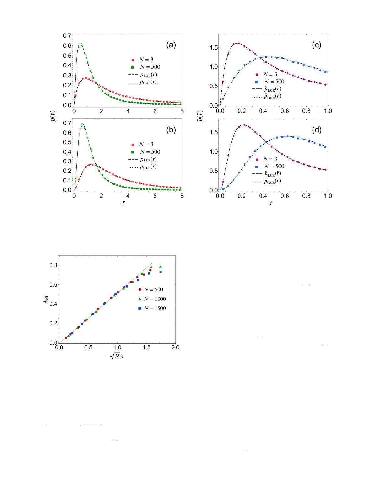
Comments & Academic Discussion
Loading comments...
Leave a Comment