Symbolic Formulae for Linear Mixed Models

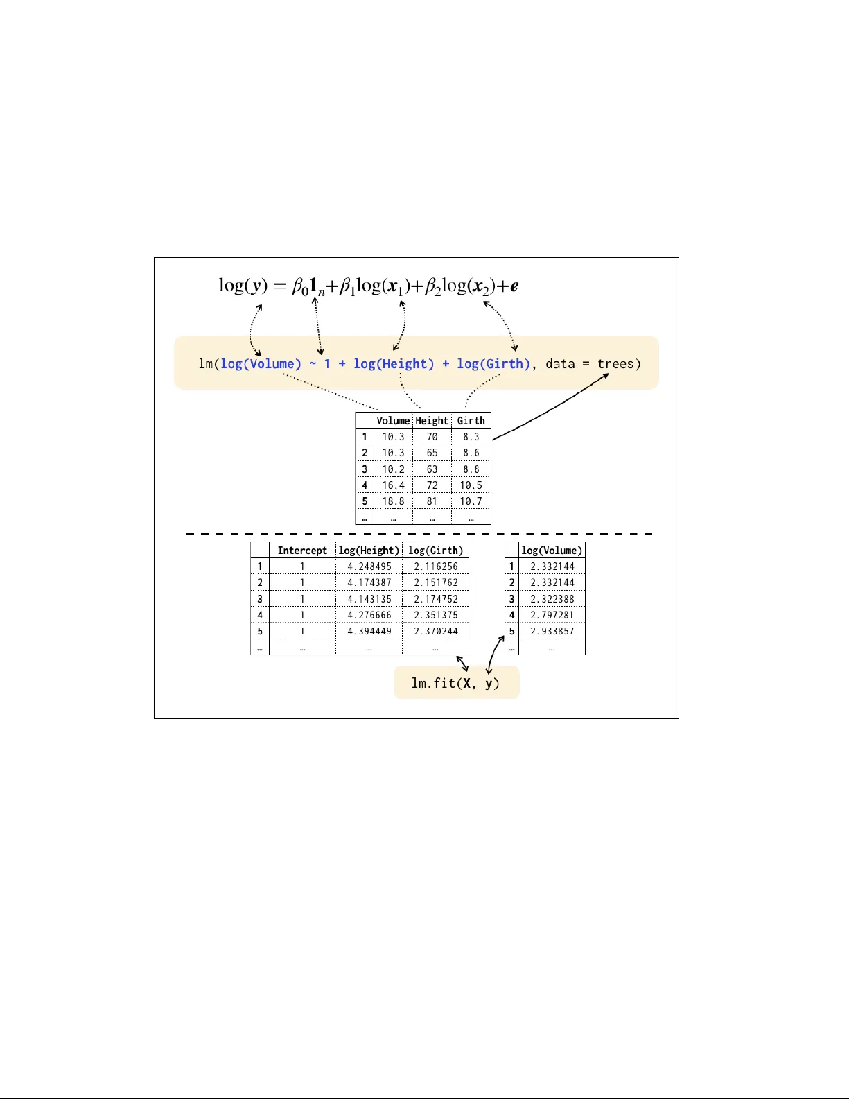
Symbolic For mulae f or Linear Mix ed Models ∗ Emi T anaka 1,2,* Francis K. C. Hui 3 1 School of Mathematics and S tatistics, The U niv ersity of Sydne y , NS W , Aus tralia, 2006 2 Depar tment of Econometrics and Business Statistics, Monash U niv ersity , VIC, A ustr alia, 3800 3 Researc h School of Finance, Actuarial Studies & S tatistics, Aus tralian N ational U niv ersity , ACT , Aus tralia, 2601 ∗ emi.tanaka@monash.edu Abs tract A statistical model is a mathematical representation of an often simpli- fied or idealised data-generating process. In t his paper, we f ocus on a par - ticular type of statistical model, called linear mixed models (LMMs), that is widely used in many disciplines e.g. agriculture, ecology , econometrics, psyc hology . Mix ed models, also commonl y known as multi-le vel, nested, hierarchical or panel data models, incor porate a combination of fixed and random effects, with LMMs being a special case. The inclusion of random effects in particular gives LMMs considerable flexibility in accounting for man y types of comple x cor related str uctures of ten f ound in dat a. This flex- ibility , how ev er, has giv en r ise to a number of wa ys b y whic h an end-user can specify the precise form of the LMM that t hey wish to fit in statistical software. In this paper, w e re vie w the softwar e design f or specification of the LMM (and its special case, t he linear model), focusing in par ticular on the use of high-lev el symbolic model f ormulae and two popular but contrasting R -packag es in lme4 and asreml . ∗ Supported by R Consor tium 1 1 Introduction Statistical models are mathematical f or mulation of often simplified real world phe- nomena, the use of whic h is ubiquitous in man y data analyses. These models are fitted or trained computationally , of ten with practitioners using some readily a v ailable application softw are packag e. In practice, statistical models in its math- ematical (or descriptive) represent ation w ould require translation to the r ight input argument to fit using an application sof tw are. The design of these input arguments (called application prog ramming interface, API) can help ease the friction in fit- ting the user’ s desired model and allo w f ocus on impor tant t asks, e.g. inter preting or using the fitted model for purposes downs tream. While there are an abundance of application sof tw are f or fitting a v ariety of sta- tistical models, the API is often inconsistent and restrictive in some f ashion. For e xample, in linear models, t he intercept ma y or ma y not be included b y default; and the random er ror typically assumed to be identical and independentl y distributed (i.i.d) wit h no option to modify these assumptions straightf orwardl y . Some effor ts ha v e been made in this front such as b y the parsnip packag e (Kuhn, 2018) in the R languag e (R Core T eam, 2018) to implement a tidy unified interface to many predictiv e modelling functions (e.g. random f orest, logistic regression, linear re- gression etc) and the scikit-learn librar y (Pedregosa et al., 2011) for machine lear ning in t he Python language (V an R ossum and Drake Jr, 1995) that provides consistent API across its modules (Buitinck et al., 2013). There is, ho we ver , little effor t on consistency or discussion f or the sof tw are specification of man y other types of statistical models, including the class of linear mix ed models (LMMs), which is the f ocus of t his ar ticle. LMMs (a special case of mixed models in general, which are also sometimes ref er red to as hierarc hical, panel data, nested or multi-lev el models) are widel y used across many disciplines (e.g. ecology , psychology , agr iculture, finance etc) due to their flexibility to model comple x, cor related str uctures in the dat a. This fle xibility is pr imar il y achiev ed via the inclusion of random effects and their cor re- sponding cov ar iance str uctures. It is this fle xibility , how ev er , that results in major differences in model specification between software f or LMMs. In R , arguabl y the most popular general pur pose pac kage to fit LMMs is lme4 (Bates et al., 2015) – total do wnloads from RStudio Comprehensiv e R Archiv e Netw ork (CRAN) mir ror from cranlogs (CsÃąrdi, 2019) indicate t here wer e ov er two million downloads f or lme4 in t he whole of 2018, while other popular mix ed model pac kages e.g. nlme , rstan , and brms (Pinheiro et al., 2019; Stan Dev elopment T eam, 2019; B Ãijrkner, 2017) in t he same year ha v e less t han half a million downloads, al- 2 beit rstan and brms are young er packag es. Another general pur pose LMM pack - age is asreml (Butler et al., 2009), which wraps the proprietar y softw are ASreml (Gilmour et al., 2009) into the R framew ork. As t his pac kage is not a vailable on CRAN, there are no comparable do wnload logs, alt hough, citations of its technical document indicates popular usage par ticularl y in the agr icultural sciences. In t his paper , we discuss only lme4 and asreml due to t heir activ e maintenance, matur ity and contrasting approaches to LMM specification. The functions to fit LMM in lme4 and asreml are lmer and asreml , respec- tiv el y . Both of these functions employ high-le v el symbolic formulae as par t of their API to specify t he model. In br ief, symbolic model formulae define t he str uctural component of a statistical model in an easier and often more accessible ter ms f or practitioners. The earlier instance of symbolic f or mulae f or linear models was ap- plied in Genstat (V SN Inter national, 2017) and GLIM (Aitkin et al., 1989), with a detailed descr iption by Wilkinson and R ogers (1973). Later on, Chambers and Hastie (1992) descr ibe t he symbolic model f ormulae implementation f or linear models in t he S language, which remains much the same in the R language. While the symbolic f ormula of linear models generally ha v e a consistent representation and e valuation r ule as implemented in stats::formula , t his is not t he case f or LMMs (and mixed models more generally) – the inconsistency of symbolic f ormu- lae ar ises pr imar ily in the representation of the random effects, with t he additional need to specify t he cov ariance structure of t he random effects as well as str ucture of the associated model matrix t hat go v erns how the random effects are mapped to (groups of) the obser v ational units. In Section 2, we br iefly descr ibe the symbolic f or mula in linear models. W e then describe the symbolic model f ormula employ ed in t he LMM functions lmer and asreml in Section 3. W e follo w b y illustrating a number of st atistical models motiv ated by t he analysis of publicl y av ailable agr icultural dat asets, with corre- sponding API for lmer and asreml in Section 4. W e limit the discussion of sym- bolic model f or mulae to mostl y those implemented in R , how e v er , it is import ant to note t hat the conceptual framew ork is not limited to this language. W e conclude with a discussion and some recommendations f or future research in Section 5. 2 Symbolic F or mulae for Linear Models A special case of LMMs is linear models, which comprises of only fix ed effects and a single random ter m (i.e. the er ror or noise), giv en in a matr ix notation as 𝒚 = 𝐗 𝜷 + 𝒆 , (1) 3 where 𝒚 is a 𝑛 -vector of responses, 𝐗 is the 𝑛 × 𝑝 design matrix with an associated 𝑝 -v ector of fixed effects coefficients 𝜷 , and 𝒆 is the 𝑛 -v ector of random er rors. T ypically we assume 𝒆 ∼ 𝑁 ( 𝟎 , 𝜎 2 𝐈 𝑛 ) . The software specification of linear model is larg ely divided into tw o approaches: (1) input of ar ray s for the response 𝒚 and design matr ix f or fixed effects 𝐗 , and (2) input of a symbolic model f ormula along wit h a data frame that define t he variables in the f or mula. The input of the data frame ma y be optional if the v ariables are defined in t he parental en vironment, although such approach is not recommended due to lar ger potential f or er ror (e.g. one variable is sor ted while others are not). Symbolic model f or mulae hav e been hea vil y used to specify linear models in R since its first public release in 1993, inher iting most of its character istic from S . In R , formulae ha ve a special class formula , and can be used f or other purposes other t han model specification, such as case_when function in dplyr R -pac kage (Wic kham et al., 2019), whic h uses t he left hand side (LHS) to denote cases to substitute with giv en value on t he r ight hand side (RHS) - t hese type of use is not within t he scope of this paper . The histor y of the formula class in R (and S ) is considerabl y longer than other popular languages, e.g. the patsy Python librar y (Smith et al., 2018), which imitates R ’ s f ormula, was introduced in 2011 and used in Statsmodels library (Seabold and Per ktold, 2010) to fit a statistical model. Symbolic model f or mulae makes use of t he v ariable names defined in the en- vironment (usually through the data frame) for specifying the precise model for - mulation. With linear models, t he LHS indicate the response; the RHS resembles its mat hematical form; and the LHS and RHS are separated by ~ which can be read as “modelled by”. For example, t he symbolic model f or mula y ~ 1 + x can be thought of as t he vector y is modelled b y a linear predictor consisting of an ov erall intercept ter m and the variable x . When the variables are numerical then the connection betw een the f ormula to its regression equation is obvious – t he LHS is 𝒚 , while the RHS cor responds to the columns of the design matr ix 𝐗 in t he linear model (1). One advantage of this symbolic model f ormula approach is t hat an y transf ormation to the variable can be parsed in the model formula and may be used later in the pipeline (e.g. prediction in its or iginal scale). This contrasts to when t he input arguments are the design matrix and t he cor responding response vector – there is now an additional step required by the user to transf or m the dat a bef ore model fitting and subsequentl y af terwards f or extrapolation. Such manual transf or mation also likel y results in manual back - transf ormation later in the anal ysis pipeline for inter pretation reasons. This no doubt creates extra lay er of fr iction for the practitioner in t heir day -to-da y analy sis. Figure 1 illustrates t his connection using the trees dat aset. 4 Figure 1: There are tw o main approaches to fitting a linear model illustrated abov e with the fit of a linear model to the trees dataset: (1) the top half uses the lm function with the input argument as a symbolic model f or mulae (in blue); (2) t he bottom half uses t he lm.fit function which requires input of design matr ix and t he response. The latter approach is not commonly used in R , how e v er , it is the com- mon approach in other languages; see Section 2.1 about t he data and t he model. 5 The specification of the intercept b y 1 in the f ormula, as done in Figure 1, is unnecessar y in R since t his is included by def ault. In turn, the remo v al of the in- tercept can be done by including -1 or +0 on the RHS. In this paper , the intercept is explicitl y included as the resemblance to its model equation form is lost without it. While the omission of 1 is long ing rained within R , we recommend to explicitl y include 1 and do not recommend designing sof tw are to requir e explicit specifi- cation to remo ve intercept as currently required in R ; see Section 2.3 f or fur ther discussion on this. Categorical or factor v ariables are typically con verted to a set of dumm y vari- ables consisting of 0s and 1s indicating whether the cor responding obser vation belongs to t he respective le v el. For parameter identifiability , a constraint needs to be applied, e.g. t he treatment constraint will estimate effects in compar ison with a par ticular reference group (the default behaviour in R ). Note that in t he presence of categorical variables, t he direct mapping of t he symbolic f ormula to the regression equation is lost. How e v er , the mapping is clear in con v erting the model equation to the so-called Analysis of V ariance (ANO V A) model specification as illustrated in Figure 2, which represents the fit of a two-w ay factorial ANO V A model to the herbicide dat a. Interaction effects are specified easily with symbolic model f ormula b y use of the : operator as seen in Figure 2. More specifically , t he f ormula in Figure 2 can also be written more compactly as sqrt(Weight) ~ 1 + Block + Population * Herbicide where the * operator is a shor thand f or including both main effects and the interaction effects. Furt her shor thand exis ts f or higher order interactions, e.g. y ~ 1 + (x1 + x2 + x3)ˆ3 is equiv alent to y ~ 1 + x1 + x2 + x3 + x1:x2 + x1:x3 + x2:x3 + x1:x2:x3 , a model that contains main effects as well as tw o-w ay and three-wa y interaction effects. The 1 can be included in the brac ke t as y ~ (1 + x1 + x2 + x3)ˆ3 to yield the same result. Perhaps sur- prisingly , y ~ (0 + x1 + x2 + x3)ˆ3 does not include t he intercept in t he fit- ted model, since 0 is con v erted to -1 and car r ied outside the bracke t and power operator . The f ormula simplification rule, say f or y ~ (0 + x1 + x2 + x3)ˆ3 , in R can be found by formula ( terms (y ~ ( 0 + x1 + x2 + x3) ^ 3 , simplify = TRUE )) ## y ~ x1 + x2 + x3 + x1:x2 + x1:x3 + x2:x3 + x1:x2:x3 - 1 6 Figure 2: In the presence of categor ical variables, t he resemblance of t he symbolic model formulae to its reg ression model f or m is not immediatel y obvious. In this case, categorical variables are transf or med to a set of dumm y variables with con- straint applied for parameter identifiability . As such, a single categor ical v ariable span a number of columns in the design matr ix. On the other hand, if the model equation is wr itten using t he ANO V A model specification (with inde x notation), then the categorical variables ha v e an immediate connection to t he fix ed effects in the model; see 2.2 f or more information about the dat a and the model. 7 2.1 T rees V olume: Linear Model The trees dat a set (or iginal dat a source from Ry an et al., 1976, built-in data in R) contain 31 obser vations with 3 numer ical v ariables. The model shown in Figure 1 is a linear model in (2) with t he 31 × 3 design matr ix 𝐗 =  𝟏 31 log( 𝒙 1 ) log( 𝒙 2 )  , where 𝒙 1 is t he tree height and 𝒙 2 is t he tree diameter (named Girth in the data). Finall y , 𝒚 is t he log of the v olume of the tree. In Figure 1, t he connection of the data column names to symbolic model f or- mula and its resemblance to the model equation is immediatel y obvious. As dis- cussed before, transf or mations ma y be sa ved f or later analy sis using t he symbolic model formulae (e.g. prediction in original scale), how e v er , this likel y requires manual recov er y when the API requires design matrix as input. 2.2 Herbicide: Categorical V ar iable The herbicide dat a set (or iginal source from R. Hull, Rothamsted Researc h, data sourced from W elham et al., 2015) cont ains 135 obser vations with 1 numer ical variable (weight response) and 3 categor ical variables: block, herbicide, and popu- lation of black -grass wit h 5, 3 and 9 le v els respectiv ely . The experiment emplo y ed has a f actorial treatment str ucture (i.e. 27 treatments which are combinations of herbicide and population), with the comple te set of treatment randomised wit hin each of the fiv e blocks (i.e. it emplo ys a randomised complete block design). The model in Figure 2 is a linear model to the square root of t he weight of the blac k -grass wit h the design matr ix 𝐗 =  𝟏 135 𝒙 1 ⋯ 𝒙 30  , where 𝒙 1 , ..., 𝒙 4 are dummy v ariables for Block B2 , B3 and B4 , 𝒙 5 , ..., 𝒙 12 are dummy v ariables f or Population P2 to P9 , 𝒙 13 and 𝒙 14 are dummy variables for Herbicide B and C , and 𝒙 15 , ..., 𝒙 30 are dummy variables for t he cor responding interaction effects. Alter nativ el y , the model can be wr itten via the ANOV A model specification, 𝑦 𝑖𝑗 𝑘 = 𝜇 + 𝛾 𝑘 + 𝛼 𝑖 + 𝛽 𝑗 + ( 𝛼 𝛽 ) 𝑖𝑗 + 𝑒 𝑖𝑗 𝑘 , where index 𝑖 deno tes f or lev el of population, index 𝑗 for le v el of herbicide and inde x 𝑘 for t he replicate block. With dummy v ariables, t he rele v ant cons traints are 𝛼 1 = 𝛽 1 = 𝛾 1 = ( 𝛼 𝛽 ) 1 𝑗 = ( 𝛼 𝛽 ) 𝑖 1 = 0 . This f or m is equiv alent to the linear regression model giv en in equation (1) with the fixed effects vector 𝜷 = ( 𝜇 , 𝛾 2 , ..., 𝛾 5 , 𝛼 2 , 𝛼 3 , ..., 𝛼 9 , 𝛽 2 , 𝛽 3 , ( 𝛼 𝛽 ) 22 , ( 𝛼 𝛽 ) 23 , ..., ( 𝛼 𝛽 ) 93 ) ⊤ . 8 2.3 Specification of intercep t Wilkinson and Rog ers (1973) descr ibed many of the operators and ev aluation r ules associated with symbolic model f or mulae, that to this day remain a mainstay of R as well as other languages. These include simplification r ules such as y ~ x + x and y ~ x:x to y ~ x . Their descr iption ho w e v er did not include an y discussion about the intercept. The symbolic ev aluation r ules gov erning t he intercept are classified as special cases in the cur rent implementation of R , alt hough t he y may not be as o v erl y intuitive on first glance, e.g. • y ~ 1:x simplifies to y ~ 1 , although one may expect y ~ x ; • y ~ 1*x simplifies to y ~ 1 , which may be surpr ising in light of t he pr o- ceeding point; • y ~ x*1 simplifies to y ~ x , which makes t he cross operator unsymme tric f or this special case. Fur ther ambiguity arises when we consider cases where we wish to explicitl y remo v e the intercept, e.g. • y ~ -1:x simplifies to the nonsensical y ~ 1 - 1 , which is equiv alent to y ~ 0 , • y ~ 1 + (-1 + x) simplifies to y ~ x - 1 . The last point w as raised b y Smith et al. (2018), and subsequently t he f ormula ev aluation differs in the patsy Python librar y on this par ticular aspect. These complications ar ise due to the e xplicit specification f or removing the intercept. Fur ther more, the symbolic model formulae t hat includes -1 or 0 remov es the re- semblance to the model equation, detracting from the aim of symbolic model for - mula to make model f ormulation straightf orward and accessible f or practitioners. It should be noted, how e v er , t hat t hese cases are all somewhat contrived and w ould rarel y be used in practice. 3 Linear Mixed Models Consider a 𝑛 -v ector of response 𝒚 , which is modelled as 𝒚 = 𝐗 𝜷 + 𝐙 𝒃 + 𝒆 , (2) where the 𝐗 is t he design matr ix f or t he fixed effects coefficients 𝜷 ; 𝐙 is the design matrix of the random effects coefficients 𝒃 , and 𝒆 is t he vector of random errors. 9 W e typically assume that the random effects and er rors are independent of eac h other and both multivariate nor mally distributed,  𝒃 𝒆  ∼ 𝑁  𝟎 𝟎  ,  𝐆 𝟎 𝟎 𝐑  where 𝐆 and 𝐑 are the cov ariance matr ices of 𝒃 and 𝒆 , respectiv el y . In Section 4, we present ex amples with different v ar iables and structures for model (2). In the next sections, we briefly descr ibe and contrast t he fitting func- tions lmer and asreml from the lme4 , asreml R -packag es, respectivel y . 3.1 lme4 The lme4 R packag e fits a LMM with the function lmer . The API consists of a sing le f ormula that extends t he linear model f ormula as f ollo w s – t he random effects are added by surrounding the ter m in round brack ets with g rouping str ucture specified on t he right of the vertical bar, and t he random ter ms within each group on the lef t of the vertical bar, e.g. (formula | group) . The formula is e v aluated under t he same mechanism for symbolic model formula as linear models in Section 2, with group specific effects from formula . These group specific effects are assumed to be nor mall y distr ibuted with zero mean and unstructured variance, as giv en abov e in (2). Examples of its use are pro vided in Section 4. 3.2 asreml In asreml , the random effects are specified as another f ormula to t he ar gument random . One of t he main strength of LMM specification in asreml , in contras t to lme4 in wide ar ray of flexible co v ariance structures. The full list of cov ariance structures av ailable in asreml V ersion 3 are given in Butler et al. (2009); asreml v ersion 4 has some slight differences as outlined in Butler et al. (2018), although the main concept is similar: v ar iance structures are specified with function-like terms in t he model f or mulae, e.g. us(factor) will fit a factor effect with un- structured co variance matr ix; diag(factor) will fit a factor effect wit h diagonal co variance matrix, i.e. zero off-diagonal and different parameterisation in the di- agonal elements. Note factor cor responds to a categor ical v ariable in the data; see Section 4 f or ex amples of its usage. 10 4 Motiv ating Examples for LMMs This section presents mo tiv ating e xamples wit h model specification b y lmer or asreml . It should be noted that the models are not advocated to be “cor rect ”, but rather a plausible model t hat a practitioner ma y consider in light of t he data and design. For succinctness, we omit all data ar gument to model fit functions. Also, this paper uses lme4 version 1.1.21; pedigreemm version 0.3.3 and asreml v ersion 3. 4.1 Chick en W eight: Longitudinal Analy sis The chick en weight data is originally sourced from Crowder and Hand (1990) and f ound as a built-in data set in R . It consists of t he weights of 50 chick ens track ed o v er regular time inter vals (not all weights at each time points are obser ved). Each chic ken are f ed one of 4 possible diets. In this experiment, we are interested in the influence of different diets on chic ken weight. W e can model the weight of each chic ken ov er time that includes diet ef- f ect, ov erall intercept and slope for time. Fitting these effects as fixed and assuming that t he er ror is i.i.d. means t hat the observations from same c hic ken are uncor re- lated and t here is no v ariation for the intercept and slope betw een chic kens. This motiv ates the inclusion of random intercept and random slope f or eac h chick en. More explicitl y , and using an ANO V A model specification, the weight ma y be modelled as 𝑦 𝑖𝑗 = 𝛽 0 + 𝛽 1 𝑥 𝑖𝑗 + 𝛼 𝑇 ( 𝑖 ) + 𝑏 0 𝑖 + 𝑏 1 𝑖 𝑥 𝑖𝑗 + 𝑒 𝑖𝑗 , (3) where 𝑦 𝑖𝑗 is t he weight of the 𝑖 -th chic ken at time index 𝑗 , 𝑥 𝑖𝑗 is t he da ys since bir th at time index 𝑗 f or the 𝑖 -th chic ken, 𝑏 0 𝑖 and 𝑏 1 𝑖 are t he random intercept and random time slope effects f or the 𝑖 -t h chic ken, 𝛽 0 and 𝛽 1 are the ov erall fix ed intercept and fix ed time slope, and 𝑒 𝑖𝑗 is the random er ror . The abov e model is incomplete without distributional assumptions f or the ran- dom effects. As intercept and slope clearly measure different units, the v ariance will be on different scales. Furt hermore, w e make an assumption that t he ran- dom intercept and random slope are cor related within t he same chic ken, but inde- pendent across chic kens. With the typical assumption of mutual independence of random effects and random error, and nor mall y and identically distributed (NID) effects, we thus ha v e the distribution assumptions,  𝑏 0 𝑖 𝑏 1 𝑖  ∼ 𝑁 𝐼 𝐷  0 0  ,  𝜎 2 0 𝜎 01 𝜎 01 𝜎 2 1  and 𝑒 𝑖𝑗 ∼ 𝑁 𝐼 𝐷 (0 , 𝜎 2 ) . (4) 11 If the effects in model (3) are vectorised as in model (2) with 𝒃 = ( 𝑏 01 , 𝑏 02 , ..., 𝑏 0 , 50 , 𝑏 11 , 𝑏 12 , ..., 𝑏 1 , 50 ) ⊤ and 𝒆 = ( 𝑒 𝑖𝑗 ) , then t he model assumption (4) can also be written as 𝒃 ∼ 𝑁  𝟎 ,  𝜎 2 0 𝜎 01 𝜎 01 𝜎 2 1  ⊗ 𝐈 𝑚  and 𝒆 ∼ 𝑁 ( 𝟎 , 𝜎 2 𝐈 𝑛 ) where ⊗ is the Kronec ker product. In asreml , a separable co variance structure, 𝚺 1 ⊗ 𝚺 2 , is specified by the use of an interaction operator where the dimensions and structures of 𝚺 1 and 𝚺 2 are specified b y t he factor input or its number of lev els and t he function that wraps the factor , e.g. us(2):id(50) is equiv alent to 𝚺 2×2 ⊗ 𝐈 50 where 𝚺 2×2 is a 2 × 2 unstr uctured cov ar iance matrix. The symbolic model f ormulae that encompasses t he model (3) coupled wit h assumption in (4) for lmer and asreml are shown in Figure 3. The two symbolic model formulae share the same syntax f or fix ed effects, ho w e v er , in this case the random effects syntax is more verbose f or asreml . One may wish to modify their assumption such that now we assume 𝒃 ∼ 𝑁  𝟎 ,  𝜎 2 0 0 0 𝜎 2 1  ⊗ 𝐈 𝑚  , That is, t he random slope and random intercept are assumed to be uncor related. This uncor related model ma y be specified in lme4 by replacing | wit h || as below . lmer (weight ~ 1 + Time + Diet + ( 1 + Time || Chick)) It should be noted that the effects specified on t he LHS of the || are uncor re- lated if t he variables are numerical only; we refer to the ex ample in T able 1 for a case where this does not w ork when t he variable is a factor . lmer (weight ~ 1 + Time + Diet + ( 1 | Chick) + ( 0 + Time | Chick)) The same model is specified as below f or asreml where now us(2) is replaced with diag(2) . The cor respondence to t he cov ar iance str ucture is more explicit, 12 Figure 3: This figure show s a longitudinal analy sis of the chick en data (see Section 4.1). The index form of the model equation sho w s direct resemblance f or symbolic model f or mula in lmer f or t he fix ed and random effects, how ev er, its cov ariance f orm is not as easily inferred. In contrast, t he symbolic model f ormula in asreml sho w resemblance of the co v ariance str ucture specified in the second argument of ~ str , how e v er , the cor responding random effects specified in the first argument of ~ str must be vectorised as show in the abo v e figure and requires implicit know l- edge of the Kronec ker product of relev ant matr ices. 13 but again inv olv es the random effects being (implicitly) vect orised as show in Fig- ure 3 and care is needed with orders of separable str ucture. asreml (weight ~ 1 + Time + Diet, random = ~ str ( ~ Chick + Chick : Time, ~ diag ( 2 ) : id ( 50 ))) 4.2 Field T rial: Co variance Structure In this example, we consider wheat yield dat a sourced from the agridat R -packag e (W right, 2018), which or iginally appeared in Gilmour et al. (1997). This dat a set consists of 𝑛 = 330 observations from a near randomised complete bloc k e xperi- ment with 𝑚 = 107 varieties, of which 3 varieties ha v e 6 replicates while the rest ha v e 3 replicates. The field trial that the yield data was collected from w as laid out in a rectangular ar ray with 𝑟 = 22 row s and 𝑐 = 15 columns. Eac h of the variety replicates are spread unif or mly to 𝑏 = 3 blocks. The columns 1-5, columns 6-10 and columns 11-15 f orm t hree equal blocks of contiguous area wit hin the field trial. The dat a frame gilmour.serpentine cont ains the columns for yield , gen (variety), rep (block), col (column) and row . Furt her columns colf and rowf , which are fact or versions of col and row , ha v e also been added. W e may model t he yield obser v ations 𝒚 , ordered by the row s within columns, using the model (2) where here 𝜷 is the 𝑏 -vect or of replicate bloc k effects and 𝒃 is the 𝑚 -v ector of variety random effects. W e consider ne xt a fe w potential co vari- ance str uctures for 𝒃 and 𝒆 . 4.2.1 Scaled identity structure. One of the simplest assumptions to make w ould be to assume t hat 𝑣𝑎𝑟 ( 𝒃 ) = 𝐆 = 𝜎 2 𝑔 𝐈 𝑚 i.e., a scaled identity str ucture. W e ma y additionally assume that 𝑣𝑎𝑟 ( 𝒆 ) = 𝜎 2 𝐈 𝑛 . In lmer , t his is fitted as below . lmer (yield ~ 0 + rep + ( 1 | gen)) T o elaborate fur ther, lmer specifies a random intercept f or eac h variety . This variety intercept will each be assumed to arise from 𝑁 𝐼 𝐷 (0 , 𝚺 1×1 ) where 𝚺 1×1 14 is a 1 × 1 unstructured variance matr ix (essentiall y a single parame ter v ariance component). The same model is fitted in asreml as belo w . Par ticularl y , idv(gen) signifies a vector of variety effects wit h idv v ariance str ucture, i.e. a scaled identity str uc- ture. This is the def ault structure in asreml , and so omitting variance str ucture, random = ~ gen , results in the same fit. asreml (yield ~ 0 + rep, random = ~ idv (gen)) 4.2.2 Crossed random effects. Field tr ials often emplo y r ow s and/or columns as blocking f actors in the e xper i- mental design. Fur t hermore, it is common practice that the manag ement practices of field experiments f ollow some systematic routine, e.g., har vesting ma y occur in a ser pentine f ashion from the first to the last ro w . These occasionall y introduce obvious un wanted noise in the dat a that are often remo v ed by including random ro w or column effects assuming that they are i.i.d. f or simplicity . These so-called crossed random effects are fitted as below f or lmer and asreml . lmer (yield ~ 0 + rep + ( 1 | gen) + ( 1 | rowf) + ( 1 | colf)) asreml (yield ~ 0 + rep, random = ~ idv (gen) + idv (rowf) + idv (colf)) 4.2.3 Error co variance structure. A field tr ial is often laid out in a rectangular array and obser vations from each plot inde x ed by row and column within this ar ra y . Consequentl y , the assumption that 𝑣𝑎𝑟 ( 𝒆 ) = 𝜎 2 𝐈 𝑛 ma y be restrictiv e when there is likel y to be some sort of spatial cor relation, i.e. plots t hat are geographically closer w ould be similar than plo ts fur ther apart. A rang e of models ma y be considered for this potential cor relation. 15 In practice, a separable autoregressiv e process of order one, denoted AR1 × AR1, has work ed well as a compromise between parsimony and flexibility as a str ucture (Gilmour et al., 1997). More specifically , we assume 𝑣𝑎𝑟 ( 𝒆 ) = 𝜎 2 𝚺 𝑐 ⊗ 𝚺 𝑟 where 𝚺 𝑐 is a 𝑐 × 𝑐 matr ix with ( 𝑖, 𝑗 ) -th entr y of 𝚺 𝑐 giv en as 𝜌  𝑖 − 𝑗  𝑐 with autocor relation parameter 𝜌 𝑐 , and a similar definition holds f or 𝑟 × 𝑟 matr ix 𝚺 𝑟 e x cept the autocor - relation parameter is denoted bvy 𝜌 𝑟 . This model is fitted in asreml by supplying a symbolic f or mula, ar1(colf):ar1(rowf) , to t he argument rcov as below . asreml (yield ~ 0 + rep, random = ~ gen, rcov = ~ ar1 (colf) : ar1 (rowf)) Here, the ar1 specifies an autoregressiv e process of order one with dimension giv en by number of lev els in rowf and colf . It is import ant to note t hat ar1 de- notes a cor relation matr ix and a cov ariance matr ix may be specified by ar1v . Care needs to be taken in cov ariance specification f or separable models, as clearl y there is a lac k of v ariance parameter(s) where 𝚺 1 and 𝚺 2 are both cor relation str uctures onl y , while if both are co v ariance structure then t he model is ov er -parameter ised and unidentifiable. In the er ror str ucture of rcov , t his is taken care of such that rcov = ~ ar1v(colf):ar1(rowf) , rcov = ~ ar1(colf):ar1v(rowf) and rcov = ~ ar1(colf):ar1(rowf) will fit all the same model. It should be noted that t his is not t he case f or separable cov ariance structures specified in random effects. In comparison, the more restr ictiv e API of lmer function does not allow the assumption on the random effects to be relaxed from 𝑣𝑎𝑟 ( 𝒆 ) = 𝜎 2 𝐈 𝑛 . One ma y of course introduce a random effect, 𝒃 𝑒 ∼ 𝑁 ( 𝟎 , 𝜎 2 𝚺 𝑐 ⊗ 𝚺 𝑟 ) , and assume 𝒆 ∼ 𝑁 ( 𝟎 , 𝜎 2 𝐈 𝑛 ) . Ho wev er, this separable co v ariance str ucture also can not be specified within lmer function. 4.2.4 Kno wn cov ariance structure. Often in plant breeding tr ials, t he varieties of interest hav e some shared ancestr y . This is captured in the f orm of pedigree data that contains 3 columns: individual ID, mother’ s ID and father’ s ID. The related str ucture is commonl y captured b y the use of a numerator relationship matr ix, denoted here has 𝐀 (Mrode, 2014). For e xample, suppose that individuals 𝑖 and 𝑗 are full-siblings. Then t he cor responding ( 𝑖, 𝑗 ) -th entry in 𝐀 is 0.5 (i.e., the a verag e probability that a randomly drawn allele from individual 𝑖 is identical b y descent to the randomly drawn allele at the same autosomal locus from individual 𝑗 ). 16 With the additional information abo v e, we ma y assume that 𝑣𝑎𝑟 ( 𝒃 ) = 𝜎 2 𝑔 𝐀 to exploit this known relatedness structure betw een varieties. The symbolic model f ormulae in lme4 alone is unable to specify this model and, an extension R package pedigreemm (V azquez et al., 2010) is required. The pedig ree data is parsed to make an object of pedigree class, which we ref er to here as ped . This object ped is then included as part of t he input in t he main fitting function pedigreemm , as depicted below . pedigreemm (yield ~ 0 + rep + ( 1 | gen), pedigree = list ( gen = ped)) In asreml , the fit is similar to t he abo ve, but the f actor with the kno wn co- variance structure must be wrapped in giv with argument ginverse pro viding a named list with the in v erse of the 𝐀 in a sparse f or mat, i.e. a data frame of 3 columns t hat consists the row and t he column inde x of 𝐀 and its cor responding value in 𝐀 provided that t he value is non-zero. asreml (yield ~ 0 + rep, random = ~ giv (gen), ginverse = list ( gen = Ainv)) 4.3 Multi-En vir onmental T rial: Separable Structure In the final e xample, we consider CIMMY T Australia ICARD A Ger mplasm Eval- uation (CAIGE) bread wheat yield 2016 data (CAIGE, 2016), which consists of 𝑡 = 7 sites across Australia, where the ov erall aim is to select the best genotype ( gen ). There were 𝑚 = 240 geno type tested across sev en tr ials and 252-391 plots, with a total of 𝑛 = 2127 yield observations. Each tr ial employ ed a partially repli- cated ( 𝑝 -rep) design (Cullis et al., 2006), wit h 𝑝 ranging from 0.23 to 0.39. Fitting a model to a model should take into account t he differential mean yield across sites, and allo w for different genotypic variations b y site. For simplicity , we ignore other v ariations f or now . In tur n, the LMM formulation in equation (2) ma y be used where 𝒚 is the v ector of yield (ordered ro w s wit hin columns within sites); 𝜷 is the 𝑡 -vector of site effects; and 𝒃 is t he 𝑚𝑡 -v ector of genotype-b y-site 17 T able 1: The table lists t he equiv alent symbolic model f or mula in lmer and asreml f or the site-by -geno type random effect, 𝒃 and t he cor responding mathematical f orm of the variance str ucture of 𝒃 . Here, 𝚺 𝑡 × 𝑡 is a 𝑡 × 𝑡 unstructured cov ariance matr ix; 𝐃 𝑡 × 𝑡 = diag ( 𝜎 2 𝑔 1 , ..., 𝜎 2 𝑔 7 ) , a 𝑡 × 𝑡 diagonal co variance matrix; 𝑚 is the number of geno types; 𝑡 is the number of sites; and S1 is a 𝑛 -vector where t he entry is one if t he cor responding obser v ation belongs to site 1 and zero other wise (similar definitions hold f or S2 , . . . , S7 ). The con v ersion of t he factor site to numerical variables S1 , ..., S7 is required to hav e uncor related random effects in lmer via the || operator, as per the last ro w in t he table. The || group separation in lmer is only effective when variables on LHS are numerical. lmer asreml 𝑣𝑎𝑟 ( 𝒃 ) idv(site):id(geno) (1 | site:geno) id(site):idv(geno) 𝜎 2 𝑔 𝐈 𝑡𝑚 site:geno (0 + site | geno) (0 + site || geno) us(site):id(geno) 𝚺 𝑡 × 𝑡 ⊗ 𝐈 𝑡 (0 + S1 + S2 + S3 + S4 + S5 + S6 + S7 | geno) (0 + S1 + S2 + S3 + S4 + S5 + S6 + S7 || geno) diag(site):id(geno) 𝐃 𝑡 × 𝑡 ⊗ 𝐈 𝑡 effects (ordered b y geno type within site). There are a number of distributions that ma y be considered f or 𝒃 , as explained belo w . W e ma y consider a separable model such that 𝒃 ∼ 𝑁 ( 𝟎 , 𝚺 𝑠 ⊗ 𝚺 𝑔 ) , where 𝚺 𝑠 and 𝚺 𝑔 are a 𝑡 × 𝑡 and 𝑚 × 𝑚 matr ices, respectivel y . W e may fur t her assume that 𝚺 𝑔 has a known str ucture similar to Section 4.2, but f or simple illustration here w e will assume that the genotypes are independent, i.e. 𝚺 𝑔 = 𝐈 𝑚 . Also, we may assume that 𝚺 𝑠 = diag  𝜎 2 𝑔 1 , 𝜎 2 𝑔 2 , ⋯ , 𝜎 2 𝑔 𝑡  , i.e. a diagonal matr ix with different v ariance paramterisation f or each site, thus allowing f or different genotypic variance at each site. This model can be fitted as below in asreml . asreml (yield ~ 0 + site, random = ~ diag (site) : id (gen)) The same model in lmer is somewhat more inv olv ed as shown in Table 1. The diagonal model assumes t hat geno type-b y -site effects are uncor related across sites f or the same geno type. How ev er , a more realistic assumption is to 18 assume that these effects are correlated, thus allowing f or different cor relation of geno type effects betw een pair of sites, i.e. w e assume that 𝚺 𝑠 is an unstructured co variance matr ix. The specification of such model f or lmer and asreml is shown in Figure 4. A ev en more realistic model may consider including site-specific random row or column effects, and assuming an AR1 × AR1 process f or the er ror cov ar iance at each site as in Section 4.2. These are easily included in asreml using the at func- tion within the symbolic model f ormulae. For ex ample, the inclusion of random ro w effect at site S1 onl y and AR1 × AR1 processes for t he er ror cov ar iance at eac h site is sho wn below . asreml (yield ~ 0 + site, random = ~ us (site) : id (gen) + at (site, "S1" ) : idv (rowf), rcov = ~ at (site) : ar1 (colf) : ar1 (rowf)) The abov e model cannot be specified using lmer . 5 Discussion In fitting statistical models, the user may not necessar y understand the full intr i- cacies of model fitting process. Ho we ver , it is essential that t he user understands ho w to specify the model that the y wish to fit and t he inter pretation from the fit. Symbolic model f ormulae is a w a y of br idging the gap between software and mat h- ematical representation of the model, and has been extensiv el y emplo y ed in R f or this pur pose. In this ar ticle, we ha v e e xtensiv el y compared tw o widel y used LMM R -packag es with contrasting model specification in functions: lmer and asreml . Bo th of these functions use symbolic model f or mulae to specify t he model wit h lmer t aking a more hierarc hical approach to random effects specification, while asreml f ocuses on the co v ariance structure of the vectorised random effects (and the dat a for t he matter). There are strength and weakness in both approac hes as w e discuss ne xt. It is clear from Section 4.1 that a random intercept and random slope model is v erbose using the symbolic model f ormulae of asreml . Specificall y , the random effect symbolic formula contains a function str t hat t akes input of tw o other for - mula: the first input specifying t he random effects, and second input specifying 19 Figure 4: Depiction of the fit of a simplified LMM for the analy sis of t he MET data. In modelling t he site -by - gen random effect, the v ariance str ucture are specified differentl y using lmer and asreml , where latter show s resemblances of cov ariance structure wr itten mathematically and when all random effects are vectorised and concatenated, while the former requires some additional computation. 20 the cov ariance structure of the vectorised f orm of random effects specified in the first input. The second input also requires the dimension(s) of co v ariance str ucture as input. These number ma y need manual update when t he data is subsequentl y updated, thus making t his symbolic model f ormula clumsy to use. On the other hand, the flexibility of asreml is e vident in Sections 4.2 and 4.3, where the LMMs fitted are less easy to pose hierarchicall y , but the v ectorised ver - sion of the LMM remains straightf orward provided one kno w s ho w to establish the set up the structure of the cov ar iance matr ices. Put another w ay , the vast set of in-built pre-defined cov ariance structures in asreml (e.g. scaled identity , di- agonal structure, unstr uctured, autoregressive process), along with the capacity to modify the er ror cov ariance str ucture and incor porate separable str uctures makes the model specification embedded in asreml a superior c hoice here. There are man y more pre-defined cov ariance str uctures not demonstrated in this paper , and interested readers may ref er to Butler et al. (2009, 2018). By contrast, the lack of fle xibility in lme4 means t hat either a more obtuse w orkaround is required or the precise LMM can not be f or mulated at all. That being said, the B Ãijrkner (2017, 2018) ( brms ) make extensiv e discussion of symbolic model f ormula and extends on the framew ork built on lme4 . The brms model f ormulae resembles lme4 and many symbolic model f ormulae in our e xamples will be similar . The brms R -packag e uses a Bay esian approach to fit its models and model specification require fur ther discussion on specifying pr iors. These discussions ar e lef t f or future revie w , although we ac kno w ledg e that suc h e xtensions may well resolv e some of the cur rent limitations of lme4 and br idge its gap in flexibility with asreml . Symbolic model formulae in R is widely used and framew orks to specify mixed models by lme4 and asreml (v ersion 3) used f or man y years. This makes dras- tic chang es difficult for these framew orks. Based on our revie w , we ar gue that ideall y any new framew ork f or symbolic model formulae should require inter- cepts to be specified explicitl y . As discussed in Section 2.3, the default inclu- sion or explicit remov al of intercepts remov es the resemblance of symbolic model f ormulae to the model equation. Cur rently , the implicit inclusion of intercepts makes cer tain model f or mulation unclear and inconsistent across different LMM specifications, e.g. (Time | Chick) in lmer includes random intercept (and slope) f or Chick , but the equivalent f or mulation str( ~ Chick + Chick:Time, ~ diag(2):id(50)) in asreml does not include the random intercept. There is a trade-off between different types of symbolic model f or mulae: lmer syntax is no doubt less flexible and may be less intuitive to some, ho we ver , with a degree of f amiliarity per t ains as a higher lev el language f or symbolic model f or- 21 mula. For many hierarc hical models, the formulation is more elegant and simpler than asreml . Howe ver , asreml is more fle xible to specify variety of cov ar iance matrices. This strength is predicated on ha ving a deeper understanding of random effects and its co variance str ucture, and promotes t he view of the LMM in a fully v ectorised f orm. A ckno w ledg ement This paper benefited from twitter conv ersation with Thomas Lumley . This paper is made using R Markdown (Xie et al., 2018). Hug e t hanks goes to t he teams behind lme4 and asreml R -packages that make fitting of general LMMs accessible to wider audiences. All mater ials used to produce this paper and its history of changes can be f ound on git hub https://git hub.com/emitanaka/ paper - symlmm . R efer ences Mur ra y Aitkin, Dorothy Anderson, Br ian Francis, and John Hinde. Statistical Modelling in GLIM . Oxford U niv ersity Press, 1989. Douglas Bates, Mar tin Machler , Ben Bolker , and Ste v e W alker . Fitting linear mix ed-effects models using lme4. Journal of Statistical Sof tw ar e , 67(1), 2015. doi: 10.18637/jss.v067.i01. Lars Buitinc k, Gilles Louppe, Mathieu Blondel, Fabian Pedregosa, Andreas Mueller , Olivier Grisel, Vlad Niculae, Peter Prettenhof er, Alex andre Gramf or t, Jaques Grobler, Robert Layton, Jake V anderPlas, Ar naud Joly , Brian Holt, and Gaël V aroquaux. API design for machine lear ning softwar e: e xperiences from the scikit-learn project. In ECML PKDD W orkshop: Languag es for Data Min- ing and Mac hine Lear ning , pages 108–122, 2013. Da vid Geoffre y Butler , Br ian R Cullis, Art hur R Gilmour, and Bev erley J Gogel. Mix ed models f or s language envir onments asreml-r reference manual, 2009. Da vid Geoffre y Butler, Bev erley J Gogel, Br ian R Cullis, and Robin Thompson. Na vigating from asreml-r v ersion 3 to 4, 2018. Paul-Christian B Ãijrkner . br ms: An r packag e for bay esian multilev el models using stan. Journal of Statistical Sof twar e , 80(1):1–28, 2017. 22 Paul-Christian B Ãijrkner . Adv anced Ba y esian Multile vel Modeling with the R P ac kage br ms. The R Journal , 10(1):395–411, 2018. doi: 10.32614/ RJ- 2018- 017. URL https://doi.org/10.32614/RJ- 2018- 017 . CAIGE. Caige project, 2016. URL http://www .caigeproject.or g.au . J.M. Chambers and T . Hastie. Statistical models in S . W adsworth & Brooks/Cole computer science series. W adsworth & Brooks/Cole A dv anced Books & Soft- w are, 1992. ISBN 9780534167646. URL http:// books.google.fr/books?id= uyfvAAAAMAAJ . M. Cro wder and D. Hand. Analysis of R epeated Measures . Chapman and Hall, 1990. URL http://www .python.org . GÃąbor CsÃąrdi. cranlogs: Download Logs from the ’RStudio’ ’CRAN’ Mirr or , 2019. URL https://CRAN.R - pr oject.org/pac kage=cr anlogs . R pac kage v ersion 2.1.1. Brian R Cullis, Alison B Smit h, and Neil Edwin Coombes. On the design of earl y generation variety tr ials with cor related dat a. Jour nal of A g ricultural, Biological, and Envir onmental Statistics , 11(4):381–393, 2006. ISSN 1085- 7117. doi: 10.1198/ 108571106X154443. Ar thur R Gilmour, Br ian R Cullis, and ArÅńnas P V erb yla. Accounting for Nat- ural and Extraneous V ariation in the Analy sis of Field Exper iments. Journal of Ag r icultur al, Biological, and Envir onmental Statistics , 2(3):269–293, 1997. doi: 10.2307/1400446. Ar thur R Gilmour, Bev erle y J Gogel, Br ian R Cullis, and R obin Thompson. AS- Reml user guide release 3.0, 2009. Max Kuhn. par snip: A Common API to Modeling and analysis F unctions , 2018. URL https://topepo.git hub.io/parsnip . R packag e version 0.0.0.9003. Raphael A Mrode. Linear Models for the Pr ediction of Animal Br eeding V alues . CABI, 3 edition, 2014. ISBN 1780643918, 9781780643915. doi: 10.1017/ CBO9781107415324.004. F . Pedregosa, G. V aroquaux, A. Gramf or t, V . Michel, B. Thir ion, O. Gr isel, M. Blondel, P . Prettenhof er , R. W eiss, V . Dubourg, J. V ander plas, A. P assos, 23 D. Cour napeau, M. Brucher , M. Per rot, and E. Duc hesna y . Scikit-lear n: Ma- chine Lear ning in Pyt hon . Journal of Mac hine Lear ning R esear c h , 12:2825– 2830, 2011. Jose Pinheiro, Douglas Bates, Saikat DebR o y , Deepay an Sarkar, and R Core T eam. nlme: Linear and Nonlinear Mixed Effects Models , 2019. URL https://CRAN. R - project.or g/pac kage=nlme . R package v ersion 3.1-140. R Core T eam. R: A Languag e and Envir onment for Statistical Com puting . R Foundation f or Statistical Computing, Vienna, Austria, 2018. URL https:// www . R - project.or g/ . T . A. R y an, B. L. Joiner , and B. F . R y an. The Minitab Student Handbook . Duxbury Press, 1976. Skipper Seabold and Josef Perktold. Statsmodels: Econometric and statistical modeling with python. In 9th Python in Science Confer ence , 2010. Nathaniel J. Smith, Christian Hudon, broessli, Skipper Seabold, P eter Quac k - enbush, Michael Hudson-Doy le, Max Humber, Katr in Lein w eber , Hassan Kibirige, Cameron Da vidson-Pilon, and Andrey Portnoy . pydata/patsy: v0.5.1, October 2018. URL https:// doi.org/10.5281/zenodo.1472929 . Stan Dev elopment T eam. RStan: the R interface to Stan , 2019. URL http: //mc- stan.or g/ . R packag e version 2.19.2. Guido V an Rossum and Fred L Drake Jr . Python tutorial . Centr um voor Wiskunde en Inf ormatica Amsterdam, The Netherlands, 1995. URL http:// www .p ython. org . A. I. V azquez, D. M. Bates, G. J. M. Rosa, D. Gianola, and K. A. W eig el. T ec h- nical note: An r packag e for fitting g eneralized linear mix ed models in animal breeding. Jour nal of Animal Science , 88:497–504, 2010. V SN Inter national. Genstat for Windo w s 19th Edition . V SN Inter national, Hemel Hempstead, UK, 2017. URL Genstat.co.uk . Sue J W elham, S A Gezan, S J Clark, and A Mead. Statistical Methods in Biology: Design and analy sis of experiments and reg ression . Chapman and Hall, 2015. 24 Hadle y Wic kham, Romain FranÃğois, Lionel Henr y , and Kirill MÃijller . dplyr: A Grammar of Data Manipulation , 2019. URL https:// CRAN.R - project.org/ pac kage=dpl yr . R pac kage v ersion 0.8.3. G N Wilkinson and C E R og ers. Symbolic descr iption of f actorial models for anal ysis of v ariance. Journal of the Royal Statistical Society: Series C (Applied Statistics) , 22(3):392–399, 1973. Ke vin W r ight. ag r idat: A g ricultural Dat asets , 2018. URL https://CRAN. R - project.or g/pac kage=agridat . R package v ersion 1.16. Yihui Xie, J.J. Allaire, and Gar rett Grolemund. R Markdo wn: The Definitive Guide . Chapman and Hall/CRC, Boca Raton, Florida, 2018. URL https: //bookdown.or g/yihui/r markdo wn . ISBN 9781138359338. 25