Invariant Solutions of the Two-Dimensional Shallow Water Equations with a Particular Class of Bottoms

The two-dimensional shallow water equations with a particular bottom and the Coriolis’s force $f=f_{0}+\Omega y$ are studied in this paper. The main goal of the paper is to describe all invariant solutions for which the reduced system is a system of ordinary differential equations. For solving the systems of ordinary differential equations we use the sixth-order Runge-Kutta method.

💡 Research Summary

The paper investigates the two‑dimensional shallow‑water equations augmented by a Coriolis term of the form (f = f_{0} + \Omega y) and a specific bottom topography (B(x,y)=q_{3}y^{4}-qy^{2}). Starting from the Eulerian form of the equations, the authors first recall that in mass‑Lagrangian coordinates the system possesses a variational structure, which allows the use of Noether’s theorem to obtain conservation laws. By exploiting equivalence transformations they set (f_{0}=0) and, through a scaling symmetry, normalize the Coriolis parameter to (\Omega=1).

The chosen bottom function corresponds to the maximal Lie‑symmetry extension found in earlier work, leading to a three‑dimensional Lie algebra (L_{3}={X_{1},X_{2},X_{3}}) with generators
(X_{1}=\partial_{t},; X_{3}=\partial_{x}) and a combined scaling‑translation generator (X_{2}) that mixes time, space and the dependent variables.

To obtain invariant solutions that reduce the original partial differential system to ordinary differential equations (ODEs), the authors construct an optimal system of two‑dimensional subalgebras of (L_{3}). Using the automorphisms of the algebra they identify three essentially different subalgebras:

1. ({X_{1},X_{3}}),
2. ({X_{2},X_{1}-2q\Omega X_{3}}),
3. ({X_{2},X_{3}}).

For each subalgebra they derive the corresponding similarity variables and reduced ODE systems.

1. Subalgebra ({X_{1},X_{3}}):
The invariance conditions imply stationary, one‑dimensional profiles (h=H(y),; u=U(y),; v=V(y)). The reduced equations lead to (U = \frac{1}{2}\Omega y^{2}+c_{2}) and a nonlinear relation among (V) and (H). The ODE for (H(y)) is highly nonlinear; the authors integrate it numerically with a sixth‑order Runge–Kutta scheme on the interval (a=1.4) to (b=-1.4) using parameters (q_{3}=5,; q=5,; \Omega=1) and initial conditions (H(a)=1,; V(a)=6,; U(a)=0). The results show that the parameter (q) strongly influences the shape of the depth profile, while the solution breaks down when the denominator in the governing ODE vanishes.

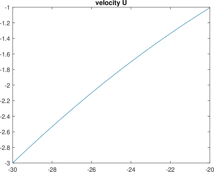
2. Subalgebra ({X_{2},X_{1}-2q\Omega X_{3}}):
Here the similarity variable is (z=(x+2q\Omega t)/y). The invariant ansatz reads (h=y^{4}H(z),; u=-2q\Omega+U(z),; v=y^{2}V(z)). The reduced system (equations (3) in the paper) contains complicated rational expressions but, remarkably, the parameter (q) disappears from the right‑hand sides. Numerical integration with initial data (H(-30)=2,; U(-30)=-3,; V(-30)=5) produces wave‑like structures reminiscent of travelling waves. Again, singularities occur when the denominator of the reduced equations becomes zero, leading to solution blow‑up.

3. Subalgebra ({X_{2},X_{3}}):
The similarity variable is (z=y,t). The invariant form is (h=t^{4}H(z),; u=-2q\Omega+t^{-2}U(z),; v=t^{-2}V(z)). The reduced ODE system (equations (4)) also lacks explicit dependence on (q). Numerical experiments with the same initial values as in case 2 show rapid growth or decay of the depth and velocity profiles, with the dynamics governed by nonlinear interactions between (H), (U) and (V). Singular behavior again appears when denominators vanish.

Across all three families, a common feature is the occurrence of finite‑time (or finite‑space) singularities where the depth (h) tends to zero or the velocities become unbounded, signalling a breakdown of the model. The analysis also reveals that the bottom‑topography parameter (q) influences only the first family of solutions; in the other two families the reduced dynamics are independent of (q).

The paper concludes that Lie‑symmetry methods combined with high‑order Runge–Kutta integration provide a systematic way to construct exact‑type invariant solutions of the shallow‑water system with Coriolis effects and non‑trivial bottom topography. These solutions, despite their idealized nature, can serve as benchmarks for more complex numerical models of geophysical flows and illustrate how symmetry reductions can uncover rich families of analytically tractable, yet physically relevant, flow patterns.