Seismic Signal Denoising and Decomposition Using Deep Neural Networks

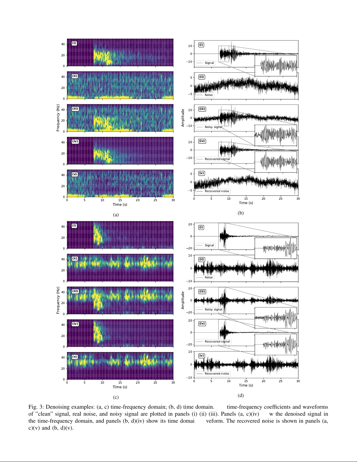
1 Seismic Signal Denoising and Decomposition Using Deep Neural Networks W eiqiang Zhu, S. Mostafa Mousa vi and Gregory C. Beroza Department of Geophysics, Stanford Uni versity Abstract —Denoising and filtering are widely used in rou- tine seismic-data-processing to impr ove the signal-to-noise ratio (SNR) of recorded signals and by doing so to improv e subsequent analyses. In this paper we de velop a new denoising/decomposition method, DeepDenoiser , based on a deep neural network. This network is able to lear n simultaneously a sparse repr esentation of data in the time-frequency domain and a non-linear function that maps this representation into masks that decompose input data into a signal of interest and noise (defined as any non- seismic signal). W e show that DeepDenoiser achieves impr essive denoising of seismic signals even when the signal and noise shar e a common frequency band. Our method properly handles a variety of colored noise and non-earthquake signals. DeepDenoiser can significantly improv e the SNR with minimal changes in the wav eform shape of interest, even in presence of high noise levels. W e demonstrate the effect of our method on impro ving earth- quake detection. There are clear applications of DeepDenoiser to seismic imaging, micro-seismic monitoring, and preprocessing of ambient noise data. W e also note that potential applications of our approach are not limited to these applications or even to earthquake data, and that our approach can be adapted to diverse signals and applications in other settings. Index T erms —seismic denoising, decomposition, deep learning, con volutional neural network I . I N T RO D U C T I O N Recorded seismic signals are inevitably contaminated by noise and non-seismic signals from various sources including: ocean waves, wind, traffic, instrumental noise, electrical noise, etc. Spectral filtering (usually based on the Fourier transform) is frequently used to suppress noise in routine seismic data processing; howe ver , this approach is not effecti ve when noise and seismic signal occupy the same frequency range. Moreov er , selecting optimal parameters for filtering is non- intuitiv e, typically varies with time, and may strongly alter the wav eform shape such that it degrades the analysis that follows. Due to these limitations, numerous efforts have been made to de velop more effecti ve noise suppression in seismic data e.g. [1, 2, 3, 4, 5, 6, 7, 8, 9, 10, 11, 12, 13, 14, 15, 16, 17, 18, 19]. Methods based on time-frequency denoising [20, 21] form a large class of seismic denoising techniques. In this approach, noisy time series are first transformed into the time- frequency domain using a time-frequency transform, such as a wav elet transform [22, 23, 24, 25, 26, 27], Short T ime Fourier T ransform (STFT) [28], S-transform [29], curvelet transform [30, 31, 32], dreamlet transform [33], contourlet zhuwq@stanford.edu transform [34], shearlet transform [35], empirical mode de- composition [36, 37, 38, 37, 39, 40], etc. The resulting time- frequency coefficients are modified (thresholded) to attenuate the coefficients associated with noise and to find an estimate of the signal coefficients. The modified coefficients are in verse transformed back into the time domain to reconstruct the denoised signal. The basic idea is to promote sparsity by transforming seismic data to other domains where the signal can be represented by a sparse set of features so that signal and noise can be separated more easily . These methods can suppress the noise e ven when it occupies the same frequency range as the signal, howe ver , the choice of a suitable thresholding function to map the noisy data into optimally denoised signal can be challenging. Denoising per- formance of time-frequency methods can be improved in two ways: either by using a more effecti ve sparse representation of the data, or by using a more flexible and powerful mapping function. Machine learning techniques, such as dictionary learning, have been used to improve seismic denoising by learning better sparse representations [41, 42, 43, 44]. The focus of this paper is on improving both sparsity and the mapping function using deep learning. Deep learning [45, 46] is a powerful machine learning technique that can learn extremely complex functions through neural networks. Deep learning has been sho wn to be a powerful tool for learning the characteristics of seismic data [47, 48, 49, 50, 51, 52, 53, 54]. In this paper we present DeepDenoiser , a nov el time- frequency denoising method using deep neural networks. This network is able to simultaneously learn a sparse representation of the input data and a high-dimensional non-linear function that maps this representation into desired masks from the training data set. Giv en an input data, DeepDenoiser pro- duces two individual masks, one for seismic signal and the other for noise signal. The masks are further used to extract the corresponding wav eforms from the input data. W e use earthquake seismograms manipulated with various types of noise and non-earthquake signals recorded by seismic stations to train the network and demonstrate its performance. W e apply the method to unseen noisy seismograms to illustrate its generalizability , to compare its performance with other denoising methods, and to document its ability to improve earthquake detection results. I I . M E T H O D In the time-frequency domain, we represent recorded data, Y ( t, f ) , as the superposition of seismic signal, S ( t, f ) , and 2 some additive natural/instrumental noise or non-seismic sig- nals, collectively termed noise, N ( t, f ) : Y ( t, f ) = S ( t, f ) + N ( t, f ) (1) The objecti ve of denoising is to estimate the underlying seismic signal (i.e., the denoised signal), ˆ S ( t, f ) , from its noise contaminated version that minimizes the expected error between the true and estimated signal: er ror = E || ˆ S ( t, f ) − S ( t, f ) || 2 2 (2) where ˆ S ( t, f ) = T F T − 1  M ( t, f ) Y ( t, f )  , T F T − 1 is the in- verse time-frequency transform, Y ( t, f ) is the time-frequency representation of noisy data, and M ( t, f ) is a function that maps Y ( t, f ) to a time-frequency representation of the esti- mated signal. Donoho and Johnstone [20] showed that this mapping can be carried out through a simple thresholding in a sparse representation where the thresholding value can be estimated from noise lev el assuming a Gaussian distribution. Here, we cast the problem as a supervised learning problem where a deep neural network will learn a sparse representation of the data to generate an optimal mapping function based on training samples of signal and noise data distribution. This is analogous to W iener decon volution as follows. W e define our mapping functions as two individual masks, M S ( t, f ) and M N ( t, f ) for signal and noise respectiv ely: M S ( t, f ) =   1 1 + | N ( t,f ) | | S ( t,f ) |   (3) M N ( t, f ) =   | N ( t,f ) | | S ( t,f ) | 1 + | N ( t,f ) | | S ( t,f ) |   (4) Each mask has the same size as the input time-frequency representation, Y ( t, f ) , and contains values between 0 and 1 that attenuate either noise or signal in time-frequency space. Inspired by the capability of auto-encoders in learning a sparse representation of data with respect to an optimization objectiv e, we designed our network in the form of a series of fully con volutional layers with descending and then ascending sizes (Fig. 1). Follo wing Ronneberger et al. [55], we use skip connections to improv e the con vergence of training and prediction performance. The inputs to the first layer are the imaginary and real parts of the time-frequency coefficients of the data, Y ( t, f ) . In the last layer masks of signal and noise ( M S ( t, f ) and M N ( t, f ) ) are provided as labels for training. The input time-frequency coefficients are processed and transformed through a series of 2D con volutional layers with a ReLU (rectified linear unit) activ ation layer and batch normalization [56]. The conv olution filter size is kept constant (3 × 3), but the feature space in the first half of the network is gradually shrunk using strides of 2 × 2. These layers act as an effecti ve feature extractor that can accelerate learning of a very sparse representation of input data at the bottleneck layer . In the second half of the network, decon volution (transpose con volution layers) are used to generate a high-dimensional non-linear mapping of this sparse representation into output masks. In the last layer, a softmax normalized exponential function is used to produce masks. Through the training process the network learns both how to construct a sparse representation of data and optimal masks to separate signal from noise by optimizing a loss function (cross-entropy loss function). Fig. 2 shows the data-flow diagram of our method. First, the seismic wa veform is transferred into the time-frequency domain. The trained network takes the real and imaginary parts of time-frequency coefficients as the input and produces individual masks for both signal and noise as the outputs. The masks are the targets in optimizing the neural network during training. The estimated time-frequency coefficients of the seismic signal, ˆ S ( t, f ) , and noise, ˆ N ( t, f ) , are obtained by applying the associated mask to the imaginary and real parts of the data coefficients, Y ( t, f ) . The final denoised signal and noise are obtained after in verse transforming ˆ S ( t, f ) and ˆ N ( t, f ) back into the time domain. Instead of defining different features and thresholds manually to enhance signal and attenuate noise, DeepDenoiser automatically learns richer features from semi-real seismic data that allo ws it to separate signal and noise in the time-frequency domain. Deep learning has the potential to provide a more effecti ve and accurate automatic denoising tool for seismic data preprocessing, which can be applied to challenging tasks such as micro-earthquake detection. I I I . N E T W O R K T R A I N I N G W e use 30-second seismograms recorded by the high broad- band channels (HN*) of the North California Seismic Network to train the neural network and test its performance. The dataset consists of 56,345 earthquake wav eforms with very high signal-to-noise ratios (SNRs) as the signal samples and 179,233 seismograms associated with various types of non- earthquake wav eforms as the noise samples. Both the signal and noise datasets are randomly split into training, v alidation and test sets. T o form ’noisy’ seismograms for training the neural network, we iterate through the signal training set repeatedly and in each iteration we add a randomly selected noise sample from the noise training set to the selected seismic signal to generate data of different SNR lev els. The Short T ime Fourier Transform (STFT) is applied to produce the time-frequency representation of the noisy wav eforms. The 2D time-frequency matrices of the noisy waveforms are the input to our deep neural network. The real and imaginary parts are fed to the neural network as two separate channels so that the network is able to learn from both the time and phase information. The prediction targets of the neural network are two masks: one each for signal and noise, composed with equation (3) and (4). The same procedure is used to generate validation and test sets. The validation set is only used for fine-tuning the hyper -parameters of the network. This helps to identify and prev ent over -fitting. The test set is used for the final results in this paper . I V . R E S U LT S A. T est Set W e use the test set to analyze the final performance and visualize the denoising results. Fig. 3 demonstrates that the 3 2x13x512 2x13x128 4x26x64 4x26x128 8x51x64 8x51x32 16x101x32 16x101 x 16 31x 201x 16 31x 201x 8 31x 201 x2 31x201x2 31x201x8 31x201x8 16x101x8 16x101x16 8x51x16 8x51x32 4x26x32 4x26x64 2x13x64 2x13x128 1x7x128 1x7x256 : Neural network layer : Skip connection : 3x3 convolution + Re lu + batch normaliza tion : 3x3 convolution + 2x2 stride + Relu + batch normaliz ation : 3x3 deconvolution + Re lu + batch n ormalizati on : 1x1 convolution + softmax Fig. 1: Neural network architecture. Inputs are the real and imaginary parts of the time-frequency representation of noisy data. Outputs are two masks for signal and noise extraction. Blue rectangles represent layers inside the neural network. The dimension of each layer is presented abov e it, and contains ”frequency bins × time points × channels”. Arrows represent different operations applied to layers. The input data first go through 3 × 3 con volution layers with 2 × 2 strides for down- sampling and then go through decon volution layers [57] for up-sampling. Batch normalization and skip connections are used to improves con vergence during training. The softmax normalized exponential function is applied in the last layer to predict the masks for signal and noise. ⨂ ⨂ (1) (4) (5) (2) (3) (6) (4) (5) (6) Time Amplitude Deep Neura l Network s Time Amplitude Time Amplitude Time Frequency Time Frequency Time Frequency Time Frequency Time Frequency Fig. 2: Data flow diagram of our denoising method. (1) The noisy data is transformed into the time-frequency domain using Short T ime Fourier T ransform (STFT). (2) The real and imaginary parts of time-frequency coef ficients are fed into our deep neural network. (3) The neural network produces two masks for signal and noise based on input data. (4, 5) The associated masks are applied to the noisy-signal coefficients to estimate the time-frequency coef ficients of the seismic signal and noise. (6) The denoised signal and noise in time domain are obtained using in verse STFT . 4 network can successfully decompose the noisy inputs with different characteristics into denoised signal and noise. The algorithm can recover denoised signal with high accuracy (Fig. 3(b, d)(iv)). As can be seen from the same example, signal leakage is minimal and the wav eform shape, frequency content, and amplitude characteristics are well preserved after denoising. These characteristics hold for the extracted noise as well (Fig. 3(b, d)(v)). One advantage of our learning-based denoising method is that the network not only learns the features of seismic signals but also the features of v arious noise. The wide variety of noise sources along with their time-v arying signatures makes it very difficult for hand-engineered features to well represent each type of noise. Howe ver , DeepDenoiser shows potential ability to learn a sparse feature representation for different types of noise. Some of them are recognized in our test dataset: The first type of noise is band-limited (Fig. 4(a, b)), with relativ ely strong values within narrow frequency bands; The second type of noise is low-frequency noise (Fig. 4(c, d))), which presents strong background fluctuations the signal rides on; The third type of noise is cyclic noise (Fig. 5), which is combined with different modes with the frequency band varying with time. The first two types of noise could be effecti vely attenuated by band-pass or low-pass filtering giv en an accurate estimate of the noise frequency bands. The third type of noise is challenging for traditional denoising methods as the noise changes with time and its frequency band overlaps with the frequency band of the target signal. For all of these types of noise, DeepDenoiser automatically predicts a mask that adapts to the noise features. The mask not only estimates the noise frequency bands needed for denoising but also reflects the changes of frequency contents ov er time. The denoised signal and the separated noise (Fig. 4(b, d)(iv , v), Fig. 5(b, d)(iv , v)) support that DeepDenoiser has robust denoising performance on various kinds of noise. W e also test DeepDenoiser on wa veforms with pure noise. Fig. 6 shows that it accurately distinguishes these waveforms from those containing earthquake signals, i.e. no recov ered signal is predicted and the recov ered noise is equiv alent to the input noise. With traditional denoising methods, the input noise wa veform on the other hand could be contaminated. This important feature renders DeepDenoiser with the ability to pre- serve noise signals with or without the presence of earthquakes at reasonable computational cost. It could have significant applications in data preprocessing for ambient seismic noise studies where the contamination of noise data with earthquake signals can heavily affect the cross-correlation results [58] and the current way of dealing with earthquake contamination is to simply discard the associated windows [59, 60]. B. Generalization The neural network is trained on seismic data that is syn- thesized by superposing real noise signals onto the real high- SNR seismic signals. T o test the network’ s generalizability , we applied it on the 91,000 samples of real seismograms recorded in Northern California. These seismograms are from detected earthquakes in the Northern California Earthquake Catalog, but are contaminated heavily by noise (Fig. 7(i)) and therefore hav e low SNRs (Fig. 8). The results suggest that DeepDenoiser successfully recovers clean seismic wav eforms (Fig. 7(ii)), e.g. the first arriv als, and improv es the SNR by around 15 dB (Fig. 8). The SNR is calculated as: SNR = 10 log 10  σ signal σ noise  (5) where σ signal and σ noise are the standard deviations of wav e- forms before and after the first arriv al. Although DeepDe- noiser is trained on synthetic data, it generalizes well to real seismograms. This suggests we can directly apply the deep neural network trained in this study to denoising tasks in real life whose performance relies on clean, undistorted seismic signals. C. Comparison with Other Methods T o compare the performance of our method with other denoising approaches, we select one seismic waveform in ”T rigger/Picker T utorial” 1 of obspy [61] as a benchmark. The wa veform is from the ”EHZ” channel, which represents a short period high gain seismometer , recorded at station R TSH of the BayernNetz (BW) Network in Germany . W e also cut a 30- second window prior to the event as the noise sample (Fig. 9). W e scale the noise wa veform to vary the noise le vel and stack it with the seismic wa veform to generate a sequence of noisy signals with varying SNRs (Fig. 9(c)). W e used normal filtering and general cross-validation de- noising [27] for the comparison. For normal filtering, we design the filter based on the smoothed frequency distribution of the clean signal (Fig. 12 in appendix), which is intended to emphasize the frequency band where the true signal resides. W e measure the SNR improvements between the denoised and noisy signals, and changes of the maximum amplitude, the correlation coefficient and the picked arriv al times as the bases of the comparison between the performance of these methods (Fig. 10). The arriv al time is picked using the same ST A/L T A method in the section below . Fig. 10 indicates that DeepDenoiser achieves a better de- noising performance while introducing smaller distortion to the signal wa veform. The SNR improvement of DeepDenoiser is more significant and more robust than the GCV method (Fig. 10(a)). Fig. 10(b) shows that DeepDenoiser recov ers the true amplitude of the signal more accurately . The max ampli- tude of the denoised signal is closer to the true signal in Fig. 9 when the SNR is larger than 2 dB, while the GCV method largely attenuates both noise and signal to achieve a good denoising performance. The higher correlation coefficients in Fig. 10(c) further demonstrates the DeepDenoiser introduces smaller wav eform distortion during denoising. In contrast, the GCV method distorts the signal wav eform significantly . DeepDenoiser is designed based on a way to separate signal and noise effecti vely , which enables it to improve SNR and preserve the signal wav eform simultaneously . The denoised wa veform also improves the recovery of arri val times from 1 https://docs.obspy .org/tutorial/code snippets/trigger tutorial.html 5 0 20 40 (i) 0 20 40 (ii) 0 20 40 Frequency (Hz) (iii) 0 20 40 (iv) 0 5 10 15 20 25 30 Time (s) 0 20 40 (v) (a) 10 0 10 Amplitude (iii) Noisy signal 10 0 10 (i) Signal 5 0 5 (ii) Noise 10 0 10 (iv) Recovered signal 0 5 10 15 20 25 30 Time (s) 5 0 5 (v) Recovered noise (b) 0 20 40 (i) 0 20 40 (ii) 0 20 40 Frequency (Hz) (iii) 0 20 40 (iv) 0 5 10 15 20 25 30 Time (s) 0 20 40 (v) (c) 20 0 20 Amplitude (iii) Noisy signal 20 0 20 (i) Signal 10 0 10 (ii) Noise 20 0 20 (iv) Recovered signal 0 5 10 15 20 25 30 Time (s) 10 0 10 (v) Recovered noise (d) Fig. 3: Denoising examples: (a, c) time-frequency domain; (b, d) time domain. The time-frequency coefficients and waveforms of ”clean” signal, real noise, and noisy signal are plotted in panels (i) (ii) (iii). Panels (a, c)(iv) show the denoised signal in the time-frequency domain, and panels (b, d)(iv) sho w its time domain wav eform. The recovered noise is shown in panels (a, c)(v) and (b, d)(v). 6 0 20 40 (i) 0 20 40 (ii) 0 20 40 Frequency (Hz) (iii) 0 20 40 (iv) 0 5 10 15 20 25 30 Time (s) 0 20 40 (v) (a) 20 0 20 Amplitude (iii) Noisy signal 20 0 20 (i) Signal 5 0 5 (ii) Noise 20 0 20 (iv) Recovered signal 0 5 10 15 20 25 30 Time (s) 5 0 5 (v) Recovered noise (b) 0 20 40 (i) 0 20 40 (ii) 0 20 40 Frequency (Hz) (iii) 0 20 40 (iv) 0 5 10 15 20 25 30 Time (s) 0 20 40 (v) (c) 10 0 10 Amplitude (iii) Noisy signal 10 0 10 (i) Signal 5 0 5 (ii) Noise 10 0 10 (iv) Recovered signal 0 5 10 15 20 25 30 Time (s) 5 0 5 (v) Recovered noise (d) Fig. 4: Denoising performance in presence of strong colored noise. It is plotted in a same manner as Fig. 3. 7 0 20 40 (i) 0 20 40 (ii) 0 20 40 Frequency (Hz) (iii) 0 20 40 (iv) 0 5 10 15 20 25 30 Time (s) 0 20 40 (v) (a) 10 0 10 Amplitude (iii) Noisy signal 10 0 10 (i) Signal 5 0 5 (ii) Noise 10 0 10 (iv) Recovered signal 0 5 10 15 20 25 30 Time (s) 5 0 5 (v) Recovered noise (b) 0 20 40 (i) 0 20 40 (ii) 0 20 40 Frequency (Hz) (iii) 0 20 40 (iv) 0 5 10 15 20 25 30 Time (s) 0 20 40 (v) (c) 10 0 10 Amplitude (iii) Noisy signal 10 0 10 (i) Signal 10 5 0 5 10 (ii) Noise 10 0 10 (iv) Recovered signal 0 5 10 15 20 25 30 Time (s) 10 5 0 5 10 (v) Recovered noise (d) Fig. 5: Denoising performance in presence of cyclic non-seismic signals. It is plotted in a same manner as Fig. 3. 8 0 20 40 (i) 0 20 40 Frequency (Hz) (ii) 0 5 10 15 20 25 30 Time (s) 0 20 40 (iii) (a) 5 0 5 (i) Noise 5 0 5 Amplitude (ii) Recovered signal 0 5 10 15 20 25 30 Time (s) 5 0 5 (iii) Recovered noise (b) 0 20 40 (i) 0 20 40 Frequency (Hz) (ii) 0 5 10 15 20 25 30 Time (s) 0 20 40 (iii) (c) 10 0 10 (i) Noise 10 0 10 Amplitude (ii) Recovered signal 0 5 10 15 20 25 30 Time (s) 10 0 10 (iii) Recovered noise (d) Fig. 6: Denoising examples of pure noise: (a, c) time-frequency domain; (b, d) time domain. The inputs are pure noise as shown in panels (i). The predicted signal masks in panels (a, c)(ii) and the recov ered signal waveforms in panels (b, d)(ii) are mostly zeros. The predicted noise masks in panels (a, c)(iii) and recovered noise wa veforms in panels (b, d)(iii) are same as the input noise in panels (i). noisy signal. With a fixed activ ation threshold for ST A/L T A method, the picked arri val times will have an sytematically increasing delay and e ventually not be recovered at increasing noise lev els. Fig. 10(d) shows that on the noisy signal the arriv al time has a delay of 0.5 s at SNR of 4 dB and fails to be recovered beyond this lev el (smaller dB). On the other hand, the denoised signal by DeepDenoiser yields an accurate arriv al time even at SNR of 2dB, which is also better than the other two denoising methods. D. Application for Earthquake Detection Background noise can significantly affect the performance of common detection algorithms such as ST A/L T A (short-term av eraging/long-term averaging) for detecting small and weak ev ents [62]. Moreover , the presence of non-earthquake signals will increase the false positive rate, and as a result, degrade detection precision. In Fig. 11 we present two examples of how DeepDenoiser can improve the ST A/L T A characteristic function. The short and long time windows are set to be 0.5 seconds and 5 seconds. Fig. 11(a) shows an example when the noise smooths out the sharp jump at the arriv al of seismic wa ves and makes the earthquake undetectable. DeepDenoiser makes this earthquake easy to detect and increases the recall rate by making the ST A/L T A characteristic function sharp after denoising. Fig. 11(b) shows another example when impul- siv e non-seismic signals bring sharp peaks to the ST A/L T A characteristic function. These peaks will be falsely detected as earthquakes by the ST A/L T A method. DeepDenoiser can effecti vely remove these non-seismic signals and increase the prediction precision. W e compare the earthquake detection results on our test dataset of 10,800 samples before and after denoising. W ith a threshold of 5, we calculate the precision of earthquake detection to be 35.14 % , 92.34 % and the recall rates to be 17.69 % , 93.76 % for the noisy signal and denoised 9 0 20 40 (i) 0 20 40 Frequency (Hz) (ii) Time (s) 0 20 40 (iii) (a) 2.5 0.0 2.5 (i) Noisy signal 2.5 0.0 2.5 Amplitude (ii) Recovered signal 0 5 10 15 20 25 30 Time (s) 2.5 0.0 2.5 (iii) Recovered noise (b) 0 20 40 (i) 0 20 40 Frequency (Hz) (ii) Time (s) 0 20 40 (iii) (c) 10 0 10 (i) Noisy signal 10 0 10 Amplitude (ii) Recovered signal 0 5 10 15 20 25 30 Time (s) 10 0 10 (iii) Recovered noise (d) Fig. 7: Denoising performance on unseen seismograms: (a, c) time-frequency domain; (b, d) time domain. The time-frequency coefficients and wav eforms of the unseen noisy signal are plotted in panels (i). Panels (a, c)(ii) show the denoised signal in the time-frequency domain, and panels (b, d)(ii) show its time domain wa veform. The recov ered noise is shown in panels (a, c)(iii) and (b, d)(iii). 0 5 10 15 20 25 30 35 40 SNR (dB) 0 2000 4000 6000 8000 10000 12000 Number Raw data Denoised data Fig. 8: Histogram showing SNR improv ement of real noisy seismograms at Northern California. signal respectively . The accuracy is defined as the ratio of true positiv e detections over the total positiv e detections. The recall rate is defined as the ratio of true positi ves over the total true number of earthquakes. Both the accuracy and recall rate are improv ed significantly by DeepDenoiser . V . D I S C U S S I O N A N D C O N C L U S I O N W e have dev eloped a novel deep-learning-based denoising algorithm for seismic data, DeepDenoiser . This learning-based approach can learn a collection of sparse features with the aim of signal and noise separation from samples of data. These features reflect more accurately the statistical characteristics of a signal of interest and can be used for effecti ve denoising or decomposition of input wav eforms. The neural network automatically determines the percentage of signal present at each data point in the time-frequency space (mask). Learning a sparse representation of data and predicting two adaptiv e thresholding masks is performed simultaneously by optimizing 10 00:19:55 00:20:00 00:20:05 00:20:10 00:20:15 00:20:20 00:20:25 Time of 2009/08/24 15 10 5 0 5 10 Amplitude (a) Signal 00:19:25 00:19:30 00:19:35 00:19:40 00:19:45 00:19:50 00:19:55 Time of 2009/08/24 2 0 2 4 Amplitude (b) Noise 0 5 10 15 20 25 30 Time (second) 10 0 10 Amplitude (c) Noisy signal Fig. 9: The wa veforms cut from ”EHZ” channel of R TSH sta- tion, BayernNetz (BW) Network in Germany: (a) the ”clean” signal; (b) the noise wa veform obtained from the same station prior to the event origin time; (c) an example of generated noisy wav eform with a stacking ratio of 3 for noise in (b) ov er signal in (a). the loss function. The masks determined by the network are then used to effecti vely decompose the input data into a signal of interest and noise. Our results show this algorithm can achie ve robust and ef- fectiv e performance in denoising of data e ven when the signal and noise share a common frequency band. The denoising ability of our method is not limited to random white noise, but performs well for a variety of colored noise and non- earthquake signals as well. Our tests indicate that DeepDe- noiser can significantly improv e the SNR with minimal change to the underlying signal of interest. DeepDenoiser preserves wa veform shape more faithfully than other denoising methods, ev en in presence of high noise levels. The network appears to be able to generalize to datasets outside of training set. W e hav e only demonstrated the capability of our method in im- proving ev ent detection; ho wev er, the potential applications of our approach are widespread. DeepDenoiser can be adapted for various types of seismic and non-seismic signals and dif ferent applications. Seismic imaging, micro-seismic monitoring, test- ban treaty monitoring, and preprocessing of ambient noise data are other potential applications of our method. Although the performance of DeepDenoiser is impressive, it does not result in a perfect separation of signal and noise. 0 2 4 6 8 10 12 0 5 10 15 20 25 30 35 SNR after denoising (dB) (a) Noisy signal Normal filtering GCV Denoising DeepDenoiser 0 2 4 6 8 10 12 10 5 0 5 10 15 Max amplitude change (b) 0 2 4 6 8 10 12 0.0 0.2 0.4 0.6 0.8 1.0 Correlation coefficient (c) 0 2 4 6 8 10 12 SNR before denoising (dB) 0.0 0.1 0.2 0.3 0.4 0.5 Arrival time change (second) (d) Fig. 10: Performance comparison between normal filtering, GCV denoising and DeepDenoiser: (a) improvement of SNR; (b) max amplitude changes; (c) correlation coefficient; (d) picked arriv al time changes. V alues in (b) and (d) are differ - ences compared with the signal in Fig. 9(a). V alues in (c) are calculated by zero-lag cross-correlation between the denoised wa veforms and the signal in Fig. 9(a). 11 10 5 0 5 10 Amplitude (i) Noisy Signal 0 5 10 15 20 25 30 Time (s) 10 5 0 5 10 Amplitude (ii) Denoised signal 0 2 4 6 8 10 (iii) STA/LTA ratio of noisy signal 0 5 10 15 20 25 30 Time (s) 0 2 4 6 8 10 (iv) STA/LTA ratio of denoised signal (a) 20 0 20 Amplitude (i) Noisy Signal 0 5 10 15 20 25 30 Time (s) 20 0 20 Amplitude (ii) Denoised signal 0 2 4 6 8 10 (iii) STA/LTA ratio of noisy signal 0 5 10 15 20 25 30 Time (s) 0 2 4 6 8 10 (iv) STA/LTA ratio of denoised signal (b) Fig. 11: Improvement of ST A/L T A characteristic function after denoising: (i) noisy signals; (ii) denoised signals; (iii) and (iv) the corresponding ST A T/L T A characteristic functions. Perfect separation of signal and noise in the time-frequency domain requires recovering two complex vectors for signal and noise from the complex vector of noisy signal, while DeepDenoiser uses the same mask for both the real and imaginary parts, and the mask, which has a v alue between [0, 1], can not recover signal values larger than the input noisy signal. Predicting the signal and noise values directly without the use of a mask may be a future direction for improvement. A C K N O W L E D G M E N T S W e thank Lind S. Gee and Stephane Zuzlewski for their help on do wnloading and processing the catalog and wav eform data from NCEDC. W e thank W illiam Ellsworth, Kaiwen W ang, Y ixiao Sheng, Kai Sheng T ai and Kexin Rong for helpful discussions. W aveform data, metadata, or data products for this study were accessed through the Northern California Earthquake Data Center (NCEDC). This research is supported by the National Science Foundation (NSF) grant number EAR- 1818579. A P P E N D I X A Frequency distrib ution of the filter used for normal filtering in the comparison section are shown in Fig. 12. This is built based on the frequency distribution of clean signal in Fig. 9(a), so that it could keep the frequency band of the clean signal. R E F E R E N C E S [1] R. Abma and J. Claerbout, “Lateral prediction for noise attenuation by tx and fx techniques, ” Geophysics , vol. 60, no. 6, pp. 1887–1896, 1995. [2] V . Oropeza and M. Sacchi, “Simultaneous seismic data denoising and reconstruction via multichannel singular spectrum analysis, ” Geophysics , vol. 76, no. 3, pp. V25–V32, 2011. [Online]. A vailable: http://library .seg.org/doi/10.1190/1.3552706 [3] D. Bonar and M. Sacchi, “Denoising seismic data using the nonlocal means algorithm, ” Geophysics , vol. 77, no. 1, pp. A5–A8, 2012. [Online]. A v ailable: http://library .seg.org/doi/10.1190/geo2011- 0235.1 [4] M. Naghizadeh, “Seismic data interpolation and denois- ing in the frequency-wav enumber domain, ” Geophysics , 12 0 10 20 30 40 50 Frequency (Hz) 0.0 0.2 0.4 0.6 0.8 1.0 Amplitude Fig. 12: Frequency distribution of the filter used for normal filtering in the comparison section vol. 77, no. 2, pp. V71–V80, 2012. [Online]. A v ailable: http://library .seg.org/doi/10.1190/geo2011- 0172.1 [5] G. Liu, X. Chen, J. Du, and K. W u, “Random noise attenuation using f-x regularized nonstationary autore- gression, ” Geophysics , vol. 77, no. 2, pp. V61–V69, 2012. [6] Y . T ian, Y . Li, and B. Y ang, “V ariable-eccentricity hyperbolic-trace tfpf for seismic random noise attenu- ation. ” IEEE T rans. Geoscience and Remote Sensing , vol. 52, no. 10, pp. 6449–6458, 2014. [7] L. Zhu, E. Liu, and J. H. McClellan, “Seismic data denoising through multiscale and sparsity-promoting dic- tionary learning, ” Geophysics , vol. 80, no. 6, pp. WD45– WD57, 2015. [8] Y . Chen and S. Fomel, “Random noise attenuation using local signal-and-noise orthogonalization, ” Geophysics , vol. 80, no. 6, pp. WD1–WD9, 2015. [9] Y . Liu, S. Fomel, and C. Liu, “Signal and noise separa- tion in prestack seismic data using velocity-dependent seislet transform, ” Geophysics , vol. 80, no. 6, pp. WD117–WD128, 2015. [10] Y . Chen, W . Huang, D. Zhang, and W . Chen, “ An open-source matlab code package for improved rank- reduction 3d seismic data denoising and reconstruction, ” Computers & Geosciences , vol. 95, pp. 59–66, 2016. [11] Y . Chen, D. Zhang, Z. Jin, X. Chen, S. Zu, W . Huang, and S. Gan, “Simultaneous denoising and reconstruction of 5-d seismic data via damped rank-reduction method, ” Geophysical Journal International , vol. 206, no. 3, pp. 1695–1717, 2016. [12] W . Huang, R. W ang, Y . Chen, H. Li, and S. Gan, “Damped multichannel singular spectrum analysis for 3d random noise attenuation, ” Geophysics , v ol. 81, no. 4, pp. V261–V270, 2016. [13] W . Huang, R. W ang, Y . Y uan, S. Gan, and Y . Chen, “Signal extraction using randomized-order multichannel singular spectrum analysis, ” Geophysics , vol. 82, no. 2, pp. V69–V84, 2016. [14] W . Huang, R. W ang, S. Zu, and Y . Chen, “Lo w-frequency noise attenuation in seismic and microseismic data us- ing mathematical morphological filtering, ” Geophysical Journal International , vol. 211, no. 3, pp. 1318–1340, 2017. [15] Y . Zhou, C. Shi, H. Chen, J. Xie, G. W u, and Y . Chen, “Spike-like blending noise attenuation using structural low-rank decomposition, ” IEEE Geoscience and Remote Sensing Letters , vol. 14, no. 9, pp. 1633–1637, 2017. [16] Y . Zhou, S. Li, D. Zhang, and Y . Chen, “Seismic noise attenuation using an online subspace tracking algorithm, ” Geophysical Journal International , vol. 212, no. 2, pp. 1072–1097, 2017. [17] Y . Chen, Y . Zhou, W . Chen, S. Zu, W . Huang, and D. Zhang, “Empirical low-rank approximation for seis- mic noise attenuation, ” IEEE T ransactions on Geoscience and Remote Sensing , v ol. 55, no. 8, pp. 4696–4711, 2017. [18] W . Huang, R. W ang, and Y . Chen, “Regularized non-stationary morphological reconstruction algorithm for weak signal detection in microseismic monitoring: methodology , ” Geophysical Journal International , vol. 213, no. 2, pp. 1189–1211, 2018. [19] Y . Chen, “Non-stationary least-squares complex decom- position for microseismic noise attenuation, ” Geophysi- cal Journal International , vol. 213, no. 3, pp. 1572–1585, 2018. [20] D. L. Donoho and J. M. Johnstone, “Ideal spatial adap- tation by wavelet shrinkage, ” biometrika , vol. 81, no. 3, pp. 425–455, 1994. [21] D. L. Donoho and I. M. Johnstone, “ Adapting to un- known smoothness via wa velet shrinkage, ” Journal of the american statistical association , vol. 90, no. 432, pp. 1200–1224, 1995. [22] S. Cao and X. Chen, “The second-generation wav elet transform and its application in denoising of seismic data, ” Applied geophysics , vol. 2, no. 2, pp. 70–74, 2005. [23] S. Gaci, “The use of wavelet-based denoising techniques to enhance the first-arriv al picking on seismic traces, ” IEEE T ransactions on Geoscience and Remote Sensing , vol. 52, no. 8, pp. 4558–4563, 2014. [24] W . Liu, S. Cao, and Y . Chen, “Seismic time-frequency analysis via empirical wa velet transform. ” IEEE Geosci. Remote Sensing Lett. , vol. 13, no. 1, pp. 28–32, 2016. [25] S. M. Mousavi, C. A. Langston, S. Mostaf a Mousavi, and C. A. Langston, “Hybrid seismic denoising using higher- order statistics and improved wa velet block threshold- ing, ” Bulletin of the Seismological Society of America , vol. 106, no. 4, pp. 1380–1393, 2016. [26] S. M. Mousavi, C. A. Langston, and S. P . Horton, “ Automatic microseismic denoising and onset detection using the synchrosqueezed con- tinuous w av elet transform, ” Geophysics , v ol. 81, no. 4, pp. V341–V355, 2016. [Online]. A vailable: http://library .seg.org/doi/10.1190/geo2015- 0598.1 [27] S. M. Mousavi and C. A. Langston, “Automatic noise-remov al/signal-removal based on general cross- validation thresholding in synchrosqueezed domain and its application on earthquake data, ” Geophysics , vol. 82, no. 4, pp. V211–V227, 2017. [Online]. A vailable: http://library .seg.org/doi/10.1190/geo2016- 0433.1 13 [28] ——, “Adaptive noise estimation and suppression for improving microseismic e vent detection, ” J ournal of Applied Geophysics , vol. 132, pp. 116–124, 2016. [Online]. A vailable: http://dx.doi.org/10.1016/j.jappgeo. 2016.06.008 [29] G.-A. Tselentis, N. Martakis, P . Paraske vopoulos, A. Lois, and E. Sokos, “Strategy for automated analysis of passiv e microseismic data based on s-transform, otsus thresholding, and higher order statistics, ” Geophysics , vol. 77, no. 6, pp. KS43–KS54, 2012. [30] G. Hennenfent and F . J. Herrmann, “Seismic denoising with nonuniformly sampled curvelets, ” Computing in Science & Engineering , vol. 8, no. 3, pp. 16–25, 2006. [31] R. Neelamani, A. I. Baumstein, D. G. Gillard, M. T . Hadidi, and W . L. Soroka, “Coherent and random noise attenuation using the curvelet transform, ” The Leading Edge , vol. 27, no. 2, pp. 240–248, 2008. [32] G. T ang and J. Ma, “ Application of total-variation-based curvelet shrinkage for three-dimensional seismic data denoising, ” IEEE geoscience and remote sensing letters , vol. 8, no. 1, pp. 103–107, 2011. [33] B. W ang, R. W u, X. Chen, and J. Li, “Simultaneous seismic data interpolation and denoising with a ne w adap- tiv e method based on dreamlet transform, ” Geophysical Journal International , vol. 201, no. 2, pp. 1180–1192, 2015. [34] H. Shan, J. Ma, and H. Y ang, “Comparisons of wav elets, contourlets and curvelets in seismic denoising, ” Journal of Applied Geophysics , vol. 69, no. 2, pp. 103–115, 2009. [Online]. A vailable: http://dx.doi.org/10.1016/j. jappgeo.2009.08.002 [35] C. Zhang and M. van der Baan, “Multicomponent mi- croseismic data denoising by 3d shearlet transform, ” Geophysics , vol. 83, no. 3, pp. A45–A51, 2018. [36] Y . Liu, Y . Li, H. Lin, and H. Ma, “ An amplitude- preserved time–frequency peak filtering based on empir- ical mode decomposition for seismic random noise re- duction, ” IEEE Geoscience and Remote Sensing Letters , vol. 11, no. 5, pp. 896–900, 2014. [37] Y . Chen and J. Ma, “Random noise attenuation by fx empirical-mode decomposition predictive filtering, ” Geophysics , vol. 79, no. 3, pp. V81–V91, 2014. [38] M. Bekara and M. V an der Baan, “Random and coherent noise attenuation by empirical mode decomposition, ” Geophysics , vol. 74, no. 5, pp. V89–V98, 2009. [39] W . Chen, J. Xie, S. Zu, S. Gan, and Y . Chen, “Multiple- reflection noise attenuation using adaptive randomized- order empirical mode decomposition. ” IEEE Geosci. Re- mote Sensing Lett. , vol. 14, no. 1, pp. 18–22, 2017. [40] J. Han and M. van der Baan, “Microseismic and seismic denoising via ensemble empirical mode decomposition and adaptive thresholding, ” Geophysics , vol. 80, no. 6, pp. KS69–KS80, 2015. [Online]. A vailable: http: //library .seg.org/doi/10.1190/geo2014- 0423.1 [41] Y . Chen, J. Ma, and S. Fomel, “Double-sparsity dictio- nary for seismic noise attenuation, ” Geophysics , vol. 81, no. 2, pp. V103–V116, 2016. [42] Y . Chen, “Fast dictionary learning for noise attenuation of multidimensional seismic data, ” Geophysical Journal International , vol. 209, no. 1, pp. 21–31, 2017. [43] M. A. N. Siahsar, S. Gholtashi, V . Abolghasemi, and Y . Chen, “Simultaneous denoising and interpolation of 2d seismic data using data-dri ven non-neg ativ e dictionary learning, ” Signal Pr ocessing , vol. 141, pp. 309–321, 2017. [44] L. Liu, J. Ma, and G. Plonka, “Sparse graph-regularized dictionary learning for suppressing random seismic noise, ” Geophysics , vol. 83, no. 3, pp. V215–V231, 2018. [45] Y . LeCun, Y . Bengio, and G. Hinton, “Deep learning, ” natur e , vol. 521, no. 7553, p. 436, 2015. [46] I. Goodfellow , Y . Bengio, A. Courville, and Y . Bengio, Deep learning . MIT press Cambridge, 2016, vol. 1. [47] P . M. DeVries, F . V i ´ egas, M. W attenberg, and B. J. Meade, “Deep learning of aftershock patterns following large earthquakes, ” Nature , vol. 560, no. 7720, p. 632, 2018. [48] T . Perol, M. Gharbi, and M. Denolle, “Conv olutional neural network for earthquake detection and location, ” Science Advances , vol. 4, no. 2, p. e1700578, 2018. [49] S. M. Mousavi, W . Zhu, Y . Sheng, and G. C. Beroza, “Cred: A deep residual network of con volutional and recurrent units for earthquake signal detection, ” arXiv pr eprint arXiv:1810.01965 , 2018. [50] Z. E. Ross, M.-A. Meier , and E. Hauksson, “P-wav e arriv al picking and first-motion polarity determination with deep learning, ” Journal of Geophysical Researc h: Solid Earth . [51] Z. E. Ross, M.-A. Meier , E. Hauksson, and T . H. Heaton, “Generalized seismic phase detection with deep learn- ing, ” arXiv pr eprint arXiv:1805.01075 , 2018. [52] Z. E. Ross, Y . Y ue, M.-A. Meier, E. Hauksson, and T . H. Heaton, “Phaselink: A deep learning approach to seis- mic phase association, ” arXiv pr eprint arXiv:1809.02880 , 2018. [53] J. Zheng, J. Lu, S. Peng, and T . Jiang, “ An automatic microseismic or acoustic emission arriv al identification scheme with deep recurrent neural networks, ” Geophysical J ournal International , v ol. 212, no. 2, pp. 1389–1397, 2018. [Online]. A vailable: http://dx.doi.org/10.1093/gji/ggx487 [54] W . Zhu and G. C. Beroza, “Phasenet: A deep-neural- network-based seismic arriv al time picking method, ” arXiv preprint arXiv:1803.03211 , 2018. [55] O. Ronneberger , P . Fischer , and T . Brox, “U-Net: Conv o- lutional Networks for Biomedical Image Segmentation, ” Miccai , pp. 234–241, 2015. [56] S. Iof fe and C. Szegedy , “Batch Normalization: Accelerating Deep Network Training by Reducing Internal Cov ariate Shift, ” 2015. [Online]. A vailable: http://arxiv .org/abs/1502.03167 [57] H. Noh, S. Hong, and B. Han, “Learning decon volution network for semantic segmentation, ” Pr oceedings of the IEEE International Confer ence on Computer V ision , vol. 2015 Inter, pp. 1520–1528, 2015. [58] X. Liu, Y . Ben-Zion, and D. Zigone, “Frequency domain analysis of errors in cross-correlations of ambient seismic 14 noise, ” Geophysical Supplements to the Monthly Notices of the Royal Astr onomical Society , vol. 207, no. 3, pp. 1630–1652, 2016. [59] G. Bensen, M. Ritzwoller , M. Barmin, A. Levshin, F . Lin, M. Moschetti, N. Shapiro, and Y . Y ang, “Processing seismic ambient noise data to obtain reliable broad- band surface wave dispersion measurements, ” Geophysi- cal Journal International , vol. 169, no. 3, pp. 1239–1260, 2007. [60] Y . Sheng, M. A. Denolle, and G. C. Beroza, “Multicomponent c3 greens functions for improved long-period ground-motion predictionmulticomponent c3 greens functions for improv ed long-period ground- motion prediction, ” Bulletin of the Seismological Society of America , vol. 107, no. 6, pp. 2836–2845, 2017. [61] M. Beyreuther , R. Barsch, L. Krischer, T . Megies, Y . Behr , and J. W assermann, “ObsPy: A Python toolbox for seismology , ” Seismological Resear ch Letters , vol. 81, no. 3, pp. 530–533, 2010. [62] M. Withers, R. Aster , C. Y oung, J. Beiriger , M. Harris, S. Moore, and J. Trujillo, “ A comparison of select trig- ger algorithms for automated global seismic phase and ev ent detection, ” Bulletin of the Seismological Society of America , vol. 88, no. 1, pp. 95–106, 1998.