Learning to Infer User Interface Attributes from Images

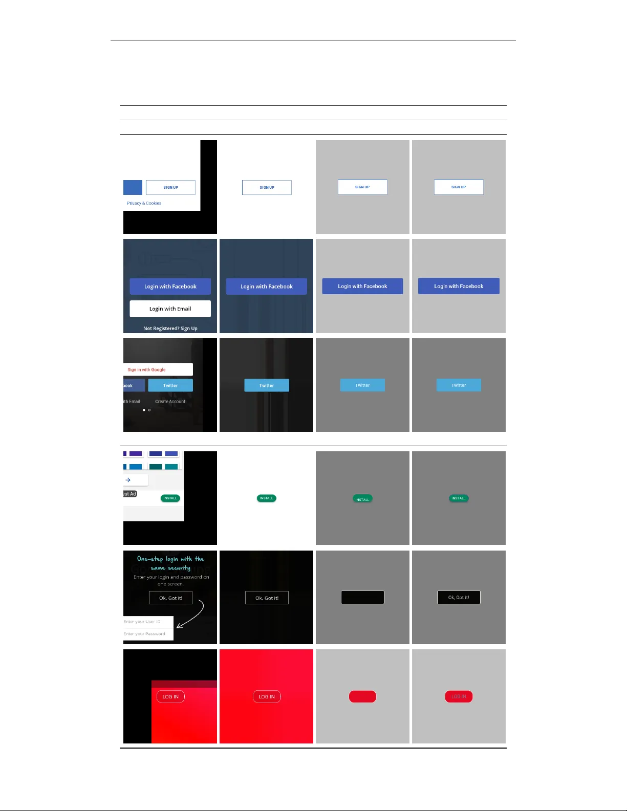
L E A R N I N G T O I N F E R U S E R I N T E R FAC E A T T R I B U T E S F R O M I M A G E S Philippe Schlattner , Pa vol Bielik & Martin V eche v Department of Computer Science ETH Z ¨ urich, Switzerland pschlatt@ethz.ch, { pavol.bielik, martin.vechev } @inf.ethz.ch A B S T R AC T W e explore a new domain of learning to infer user interface attributes that helps dev elopers automate the process of user interface implementation. Concretely , giv en an input image created by a designer, we learn to infer its implementation which when rendered, looks visually the same as the input image. T o achie ve this, we take a black box rendering engine and a set of attributes it supports (e.g., colors, border radius, shado w or text properties), use it to generate a suitable synthetic training dataset, and then train specialized neural models to predict each of the attribute v alues. T o improve pixel-le vel accuracy , we also use imitation learning to train a neural policy that refines the predicted attribute values by learning to compute the similarity of the original and rendered images in their attribute space, rather than based on the dif ference of pix el values. W e instantiate our approach to the task of inferring Android Button attribute values and achieve 92.5% accuracy on a dataset consisting of real-world Google Play Store applications. 1 I N T RO D U C T I O N W ith over 5 million applications in Google Play Store and Apple App Store and ov er a billion webpages, a significant amount of time can be saved by automating ev en small parts of their de- velopment. T o achiev e this, sev eral tools have been recently dev eloped that help user interface designers explore and quickly prototype different ideas, including Sketch2Code (Microsoft, 2018) and InkToCode (Corrado et al., 2018), which generate user interface sketches from hand-drawn images, Swire (Huang et al., 2019) and Rico (Deka et al., 2017), which allo w retrieving designs similar to the one supplied by the user and Rewire (Swearngin et al., 2018), which transforms im- ages into vector representations consisting of rectangles, circles and lines. At the same time, to help dev elopers implement the design, a number of approaches hav e been proposed that generate layout code that places the user interface components at the desired position (e.g., when resizing the application). These include both symbolic synthesis approaches such as InferUI (Bielik et al., 2018), which encodes the problem as a satisfiability query of a first-order logic formula, as well as statistical approaches (Beltramelli, 2018; Chen et al., 2018), which use encoder-decoder neural networks to process the input image and output the corresponding implementation. In this work, we explore a new domain of inferring an implementation of an user interface compo- nent from an image which when rendered, looks visually the same as the input image. Going from an image to a concrete implementation is a time consuming, yet necessary task, which is often out- sourced to a company for a high fee (replia, 2019; psd2android, 2019; psd2mobi, 2019). Compared to prior work, we focus on the pixel-accurate implementation, rather than on producing sketches or the complementary task of synthesizing layouts that place the components at the desired positions. Concretely , given a black box rendering engine that defines a set of categorical and numerical at- tributes of a component, we design a two step process which predicts the attribute values from an input image – (i) first, we train a neural model to predict the most likely initial attribute values, and then (ii) we use imitation learning to iterativ ely refine the attribute v alues to achiev e pixel-le vel accu- racy . Crucially , all our models are trained using synthetic datasets that are obtained by sampling the black box rendering engine, which makes it easy to train models for other attrib utes in the future. W e instantiate our approach to the task of inferring the implementation of Android Button attributes 1 and sho w that it generalizes well to a real-world dataset consisting of buttons found in e xisting Google Play Store applications. In particular , our approach successfully infers the correct attribute values in 94.8% and 92.5% of the cases for the synthetic and the real-w orld datasets, respectiv ely . 2 R E L A T E D W O R K As an application, our work is related to a number of recently dev eloped tools in the domain of user interface design and implementation with the goal of making dev elopers more productiv e, as discussed in Section 1. Here we give o vervie w of the related research from a technical perspective. In verting rendering engines to interpr et images The most closely related work to ours phrases the task of inferring attrib utes from images as the more general task of learning to in vert the render- ing engines used to produce the images. For example, W u et al. (2017) use reinforcement learning to train a neural pipeline that given an image of a cartoon scene or a Minecraft screenshot, identifies objects and a small number of high lev el features (e.g., whether the object is oriented left or right). Ganin et al. (2018) also use reinforcement learning, but with an adversarially learned reward signal, to generate a program ex ecuted by a graphics engine that dra ws simple CAD programs or handwrit- ten symbols and digits. Johnson et al. (2018) and Ellis et al. (2018) design a neural architecture that generates a program that when rendered, produces that same 2D or 3D shape as in the input image. While Johnson et al. (2018) train the network using a combination of supervised pretraining and re- inforcement learning with a custom reward function (using Chamfer distance to measure similarity of tw o objects), Ellis et al. (2018) use a tw o step process that first uses supervised learning to predict a set of objects in the image and then synthesizes a program (e.g., containing loops) that draws them. In comparison to these prior works, our approach dif fers in three key aspects. First, the main chal- lenge in prior works is predicting the set of objects contained in the image and ho w to compose them. Instead, the focus of our work is in predicting a set of object properties after the objects in the image were already identified. Second, instead of using the expensi ve REINFORCE (W illiams, 1992) algorithm (or its v ariation) to train our models, we use a two step process that first pretrains the network to make an initial prediction and then uses imitation learning to refine it. This is pos- sible because, in our setting, there is a fixed set of attributes known in advance for which we can generate a suitable synthetic dataset used by both of these steps. Finally , because our goal is to learn pixel-accurate attribute v alues, the refinement loop takes as input both the original image, as well as the rendered image of the current attribute predictions. As a result, we do not require our models to predict pixel-accurate rendering of an attribute value b ut instead, to only predict whether the attribute v alues in two images are the same or in which direction they should be adjusted. Attribute prediction Optical character recognition (Jaderberg et al., 2016; L yu et al., 2018; Jader - berg et al., 2014; Gupta et al., 2016) is a well studied example of predicting an attribute from an image with a lar ge number of real-world applications. Other examples include predicting text fonts (Zhao et al., 2018; W ang et al., 2015; Chen et al., 2014), predicting eye gaze (Shriv astav a et al., 2017), face pose and lighting (Kulkarni et al., 2015), chair pose and content (W u et al., 2018) or 3D object shapes and pose (Kundu et al., 2018), to name just a few . The attribute prediction network used in our work to predict the initial attribute v alue is similar to these e xisting approaches, except that it is applied to a new domain of inferring user interface attrib utes. As a result, while some of the challenges remain the same (e.g., how to ef fectiv ely generate synthetic datasets), our main challenge is designing a pipeline, together with a network architecture capable of achieving pixel-le vel accuracies on a range of div erse attributes. 3 B A C K G RO U N D : U S E R I N T E R FAC E A T T R I B U T E S V isual design of user interface components can be specified in many different ways – by defining a program that draws on a can vas, by defining a program that instantiates components at runtime and manipulates their properties, declarati vely by defining attribute values in a configuration file (e.g., using CSS), or by using a bitmap image that is rendered in place of the components. In our work, we follow the best practices and consider the setting where the visual design is defined declarati vely , thus allowing separating the design from the logic that controls the application beha viour . 2 Formally , let C denote a component with a set of attributes A . The domain of possible v alues of each attribute a i ∈ A is denoted as Θ i . As all the attributes are rendered on a physical device, their domains are finite sets containing measurements in pixels or a set of categorical values. For example, the domain for the text color attribute is three RGB channels N 3 × [0 , 255] , the domain for text gravity is { top , left , center , right , bottom } and the domain for border width is N [0 , 20] . W e distinguish two domain types: (i) comparable (e.g., colors, shadows or sizes) for which a v alid distance metric d : Θ × Θ → N [0 , ∞ ) exists, and (ii) uncomparable (e.g., font types or text gravity) for which the distance between any two attribute v alues is equal to one. W e use Θ ⊆ Θ 1 × · · · × Θ n to denote the space of all possible attrib ute configurations, and use the function render : Θ → R 3 × h × w to denote an image with width w , height h and three color channels obtained by rendering the attribute configuration y ∈ Θ . Furthermore, we use the notation y ∼ Θ to denote a random sample of attribute v alues from the space of all valid attribute configurations. Finally , we note that attributes often affect the same parts of the rendered image (e.g., the shadow is o verlayed on top of the background) and they are in general not independent of each other (e.g, changing the border width affects the border radius). 4 L E A R N I N G T O I N F E R U S E R I N T E R F AC E A T T R I B U T E S F R O M I M A G E S W e now present our approach for learning to infer user interf ace component attrib utes from images. Problem statement Given an input image I ∈ R 3 × h × w , our goal is to find an attribute configura- tion y ∈ Θ which when rendered, produces an image most visually similar to I : arg min y ∈ Θ cost ( I , render ( y )) (1) where cost : I × I → R [0 , ∞ ) is a function that computes the visual similarity of a giv en user interface component in two images. It returns zero if the component looks visually the same in both images or a positiv e real value denoting the degree to which the attrib utes are dissimilar . The first challenge that arises from the problem statement abov e is ho w to define the cost function. Pixel based metrics, such as mean squared error of pixel differences, are not suitable and instead of producing images with similar attrib ute values, produce images that hav e on av erage similar colors. T raining a discriminator also does not work, as all the generated images are produced by rendering a set of attributes and are true images by definition. Finally , the cost can be computed not ov er the rendered image but by comparing the predicted attributes y with the ground-truth labels. Unfortunately , e ven if we would spend the ef fort and annotated a large number of images with their ground-truth attributes, using a manually annotated dataset restricts the space of models that can be used to infer y to only those that do supervised learning. In what follows we address this challenge by showing how to define the cost function ov er attributes (used for supervise learning) as well as ov er images (used for reinforcement learning), both by using a synthetically generated dataset. Our approach T o address the task of inferring user interface attrib utes from images, we propose a two step process that – (i) first selects the most lik ely initial attribute values arg max y ∈ Θ p ( y | I ) by learning a probability distribution of attribute values conditioned on the input image, and then (ii) iterativ ely refines the attribute v alues by learning a polic y π (∆ y ( i ) | I , render ( y ( i ) )) that represents the probability distribution of how each attribute should be changed, conditioned on both the original image, as well as the rendered image of the attribute configuration y ( i ) at iteration i . W e use the policy π to define the cost between two images as cost ( I , I 0 ) : = 1 − π (∆ y = 0 | I , I 0 ) . That is, the cost is defined as the probability that the two images are not equal in the attrib ute space. W e illustrate both steps in Figure 1 with an example that predicts attrib utes of a Button component. In Figure 1 (a) , the input image is passed to a set of con volutional neural networks, each of which is trained to predict a single attribute v alue. In our example, the most likely value predicted for the border width is 2dp while the most likely color of the border is # 4a4a4a . Then, instead of returning the most likely attribute configuration y , we take advantage of the fact that it can be rendered and compared to the original input image. This giv e us additional information that is used to refine the predictions as shown in Figure 1 (b) . Here, we use a pair of siamese networks (pre- trained on the prediction task) to learn the probability distribution over changes required to make the component attributes in both images the same. In our example, the network predicts that the border 3 (a) Attribute Prediction (Section 4.1) CNN CNN y border width 2dp border color shadow 0dp text gravity center . . . p ( y | I ) 0 . 77 0 . 99 0 . 91 0 . 96 D =  render ( y ( i ) ) , y ( i ) ∼ Θ  N i =1 T raining Input Image I p ( y | I ) Predicted Attributes render ( y ) (b) Attribute Refinement Loop (Section 4.2) CNN CNN CNN CNN Siamese Networks ∆ y ( i ) border width − 2dp 0 . 67 border color 0 0 . 99 shadow + 4dp 0 . 61 text gravity 0 0 . 98 . . . ∆ y ∼ π (∆ y ( i ) 6 = 0 | I , render ( y ( i ) )) y 0 = y ( i ) + ∆ y y ( i +1) = arg min y ∈{ y ( i ) , y 0 } cost ( I , render ( y )) D ∆ =  h render ( y ( i ) ∼ Θ ) , render ( y ( j ) ∼ Θ ) i , ∆( y ( i ) − y ( j ) )  M i,j =1 T raining Input Image I render ( y ( i ) ) π (∆ y ( i ) | I , render ( y ( i ) )) Predicted Changes Select & Apply Change Accept or Reject Change Figure 1: (a) Illustration of the attribute prediction network which takes an input an image with a component (a Button ) and predicts all the component attribute values. (b) Refinement loop which renders the attribute v alues obtained from (a) and iteratively refines them to match the input image. color and the text gravity attributes have already the correct values but the border width should be decreased by 2dp and the shadow should be increased by 4dp . Then, due to the large number of dif ferent attributes that affect each other , instead of applying all the changes at once, we select and apply a single attribute change. In our example, the ∆ y corresponds to adjusting the v alue of border width by − 2dp . Since the change is supposed to correct a mispredicted attrib ute value, we accept it only if it indeed makes the model more confident that the prediction is correct. Synthetic datasets W e instantiate our approach by training it purely using synthetic datasets, while ensuring that it generalizes well to real-world images. This allows us to av oid the expen- siv e task of collecting and annotating real-world datasets and more importantly , makes our approach easily applicable to ne w domains and attrib utes. In particular, gi ven a space of possible attribute configurations Θ and a rendering function render , we generate two different datasets D and D ∆ used to train the attribute prediction network and the policy π , respecti vely . The dataset D = { ( render ( y ( i ) ) , y ( i ) ∼ Θ ) } N i =1 is constructed by sampling a valid attribute configuration y ( i ) ∼ Θ and rendering it to produce the input image. T o generate D ∆ , we sample two attribute configurations y ( i ) , y ( j ) ∼ Θ that are used to render two input images and train the network to predict the difference of their attrib utes, that is, D ∆ = { ( h render ( y ( i ) ∼ Θ ) , render ( y ( j ) ∼ Θ ) i , ∆( y ( i ) − y ( j ) )) } M i,j =1 . For both datasets, to av oid ov erfitting when training models for attributes with lar ge domain of possible v alues, we sample only a subset of attributes, while setting the remaining attributes to values from the previous example y ( i − 1) . As a result, ev ery two consecutiv e samples are similar to each other , since a subset of their attributes is the same. Further , because the real-world images do not contain components in isolation but together with other components that fill the rest of the screen, we introduce three additional attrib utes x pos ∈ N , y pos ∈ N and background . W e use x pos and y pos to denote the horizontal and vertical position of the component in the image, respecti vely . This allo ws the network to learn robust predictions regardless of the component position in the image. W e use background to select the background on which the component is rendered. W e experimented with three different choices of backgrounds – only while color , random solid color and overlaying the component on top of an existing application, all of which are e valuated in Section 5. 4 4 . 1 A T T R I B U T E P R E D I C T I O N The attribute prediction network architecture is a multilayer con volutional neural network (CNN) followed by a set of fully connected layers. The multilayer conv olutional part consists of 6 repeti- tiv e sequences of con volutional layers with ReLU acti vations, follo wed by batch normalization and a max-pooling layer of size 2 and stride 2. For the con volutional layers we use 3 × 3 filters of size 32, 32, 64, 64, 128 and 128, respectiv ely . The result of the con volutional part is then flattened and connected to a fully connected layer of size 256 with ReLU activ ation followed by a final softmax layer (or a single neuron for regression). W e note that this is not a fixed architecture and instead, it is adapted to a giv en attribute by performing an architecture search, as shown in Section 5. Supporting multiple inp ut sizes T o support user interf ace components of different sizes, we select the input image dimension such that it is large enough to contain them. This is necessary as our goal is to infer pix el-accurate attribute v alues and scaling down or resizing the image to a fixed dimension is not an option, as it leads to se vere performance degradation. Howe ver , this is problematic, as most of the input images are smaller or cropped in order to remov e other components. As a result, before feeding the image to the network we need to increase the dimension of the input without resizing or scaling. T o achiev e this, we pad the missing pixels with the v alues of edge pixels, which improv es the generalization to real-world images as sho wn in Section 5.1 and illustrated in Appendix C. Optimizations T o improv e the accuracy and reduce the variance of the attribute prediction network, we perform the following two optimizations. First, we compute the most likely attrib ute value by combining multiple predictions and selecting the most likely among them. This is achieved by generating sev eral perturbations of the input image, each of which shifts the image randomly , horizontally by  x ∼ U ( − t, t ) and vertically by  y ∼ U ( − t, t ) , where t ∈ N . This is similar to ensemble models but instead of training multiple models we generate and e valuate multiple inputs. Second, to improve the accuracy of the color attributes, we perform color clipping by picking the closest color to one of those present in the input image. T o reduce the set of all possible colors, we use saliency maps (Simonyan et al., 2013) to select a subset of the pixels most relev ant for the prediction. In our experiments we keep only the pixels with the normalized saliency value above 0.8. Then, we clip the predicted color to the closest color from the top fi ve most common colors among the pix els selected by the salienc y map. W e provide illustration of the color clipping in Appendix D. 4 . 2 A T T R I B U T E R E FI N E M E N T L O O P W e now describe how to learn a function π (∆ y | I , render ( y )) that represents probability distri- bution of how each attribute should be changed, conditioned on both the original image as well as the rendered image of the current attribute configuration y . W e can think of π as a policy , where the actions correspond to changing an attribute value and the state is a tuple of the original and the currently rendered image. W e can then apply imitation learning to train the policy π on a synthetic dataset D ∆ = { ( h render ( y ( i ) ∼ Θ ) , render ( y ( j ) ∼ Θ ) i , ∆( y ( i ) − y ( j ) )) } M i,j =1 . Because the range of possible v alues ∆( y ( i ) − y ( j ) ) can be large and sparse, we limit the range by clipping it to an interval [ − c, c ] (where c is a hyperparameter set to c = 5 for all the attributes in our ev aluation). T o fix a change larger than c , we perform sequence of small changes. For comparable attributes, the delta between two attrib ute values is defined as their distance ∆( y ( i ) k − y ( j ) k ) : = d ( y ( i ) k − y ( j ) k ) . For uncomparable attributes, the delta is binary and determines whether the v alue is correct or not. The model architecture used to represent π consists of two con volutional neural networks with shared weights θ , also called siamese neural networks, each of which computes a latent represen- tation of the input image h x = f θ ( I ) and h r = f θ ( render ( y )) . The function f θ has the same architecture as the attribute prediction network, except that we replace the fully connected layer with one that has a bigger size and remo ve the last softmax layer . Then, we combine the latent features h x and h r into a single vector h = [ h x ; h r ; h x + h r ; h x − h r ; h x  h r ] , where  denotes element-wise multiplication. Finally , the vector h is passed to a fully connected layer of size 256 with ReLU activ ations, followed by a final softmax layer . Once the models are trained, we perform the refinement loop as follows: Select attrib ute to chang e . As in general attrib utes interfere with each other , in each refinement iter - ation we adjust only a single attribute, which is chosen by sampling from the follo wing distribution: 5 P [ A = a i ] = 1 − π (∆ y i = 0 | I , render ( y )) P |A| k =1 1 − π (∆ y k = 0 | I , render ( y )) (2) where π (∆ y k = 0 | I , render ( y )) denotes the probability that the k -th attribute should not be changed, that is, the predicted change is zero. Since we train a separate model for each attrib ute, the probability that the giv en attribute should be changed is 1 − π (∆ y k = 0 | I , render ( y )) . Select attribute’ s new value . For comparable attributes, we adjust their v alue by sampling from the probability distribution computed by the policy π , which contains changes in range [ − c, c ] . For uncomparable attributes another approach has to be chosen, since the delta prediction network computes only whether the attribute is correct and not how to change it. Instead, we select the new value by sampling from the probability distribution computed by the corresponding attrib ute prediction network. Accept or reject the change . In a typical setting, we would accept the proposed changes as long as the model predicts that an attribute should be changed. Howe ver , in our domain we can render the proposed changes and check whether the result is consistent with the model. Concretely , we accept the change y 0 if it reduces the cost , that is, cost ( I , render ( y 0 )) < cost ( I , render ( y )) . Note that this optimization is possible only if the change was supposed to fix the attribute value, that is, the change was in the range ( − c, c ) or the attrib ute is uncomparable. 5 E V A L U A T I O N T o ev aluate the effecti veness of our approach, we apply it to the task of generating Android Button implementations. Concretely , we predict the following 12 attributes – border color, border width, border radius, height, width, padding, shadow , main color , text color , text font type, te xt gravity and text size. W e do not predict the text content for which specialized models already exist (Jaderberg et al., 2016; L yu et al., 2018; Jaderber g et al., 2014; Gupta et al., 2016). W e pro vide domains and the visualization of all these attrib utes in Appendix A. In what follo ws we first describe our datasets and ev aluation metrics, then we present a detailed e valuation of our approach consisting of the attrib ute prediction network (Section 4.1) and the refinement loop (Section 4.2). Datasets T o train the attribute prediction network we use a synthetic dataset D containing ≈ 20,000 images and their corresponding attributes as described in Section 4. T o train the refinement loop we use a second synthetic dataset D ∆ , also containing ≈ 20,000 image pairs. During training we perform two iterations of DAgger (Ross et al., 2011), each of which generates ≈ 20,000 samples obtained by running the policy on the initial training dataset. T o e valuate our models we use two datasets – (i) synthetic D sy n generated in the same way as for training, and (ii) real-world D g play we obtained by manually implementing 110 buttons in e xisting Google Play Store applications. The il- lustration of samples and our inferred implementations for both datasets are provided in Appendix F. Evaluation metrics T o remove clutter, we introduce an uniform unit to measure attribute similar - ity called per ceivable differ ence . W e say that two attributes have the same ( = ) perceiv able difference if their v alues are the same or almost indistinguishable. For e xample, the te xt size is percei vably the same, if the distance of the predicted y and the ground-truth y ∗ value is d ( y , y ∗ ) ≤ 1 , while the border width is perceiv ably the same only if it is predicted perfectly , i.e., d ( y , y ∗ ) = 0 . The formal definition of perceiv able difference with visualizations of all attrib utes is provided in Appendix E. 5 . 1 A T T R I B U T E P R E D I C T I O N A detailed summary of the variations of our attribute prediction models and their effect on perfor- mance is shown in T able 1. T o enable easy comparison, we selected a good performing instantiation of our models, denoted as cor e , against which all variations in the rows (A)-(E) can be directly compared. Based on our experiments, we then select the best configuration that achiev es accuracy 93 . 6% and 91 . 4% on the synthetic and the real-world datasets, respecti vely . All models were trained for 500 epochs, with early-stopping of 15 epochs, using a batch size of 128 and initial learning rate of 0.01. In what follows we provide a short discussion of each of the v ariations from T able 1. 6 T able 1: V ariations of the attrib ute prediction network and their ef fect on the model accuracy . Network Architecture Dataset & Input Preprocessing Accuracy ar ch lr rd color clip input size tr back g r ound D syn = D gplay = cor e C 0 ,R 0 - sal iency top 5 150 × 330 tr 2 r and 92.7% 90.1% ( A ) white 88.9% 56.7% scr eenshot 88.6% 75.6% ( B ) center 89.4% 82.4% tr 1 92.3% 90.3% ( C ) 135 × 310 92.5% 91.2% 180 × 350 92.5% 88.7% ( D ) imag e top 5 89.2% 85.9% imag e all 87.1% 83.0% none 74.1% 72.0% ( E ) C 3 83.2% 83.4% C 6 88.6% 88.2% R 1 62.6% 64.3% R 2 67.7% 65.3% b est C 6 , R 2 0 . 1 saliency top 5 135 × 310 tr 2 r and 93.6% 91.4% ar ch model architecture tr input transformation lr rd reduced learning rate on plateau Image backgr ound (A) W e trained our models on synthetic datasets with three dif ferent component backgrounds of increasing complexity – white color , random solid color and user interface screen- shot. Unsurprisingly , the models trained with white background fail to generalize to real-world datasets and achieve only 56 . 7% accuracy . Perhaps surprisingly , although the models trained with the screenshot background impro ve significantly , the y also fail to generalize and achie ve only 75 . 6% accuracy . Upon closer inspection, this is because overlaying components ov er existing images often introduces small visual artefacts around the component. On the other hand, random color back- grounds generalize well to real-world dataset as they ha ve enough variety and no visual artef acts. Affine tr ansformations (B) Since the components can appear in an y part of the input image, we use three methods to generate the training datasets – tr 1 places the component randomly at an y position with a margin of at least 20 pixels of the image border, tr 2 places the component in the middle of the image with a horizontal of fset  x ∼ U ( − 13 , 13) and vertical of fset  y ∼ U ( − 19 , 19) , and center always places the component exactly in the center . W e can see that using either tr 1 or tr 2 leads to significantly more robust model and increases the real-w orld accuracy by ≈ 8% . Input image size & padding (C) As our goal is to perform pixel-accurate predictions, we do not scale down or resize the input images. Howe ver , since large images include additional noise (e.g., parts of the application unrelated to the predicted component), we measure how rob ust our model is to such noise by training models for three dif ferent input sizes – 135 × 310 , 150 × 330 and 180 × 350 . While the accurac y on the synthetic dataset is not affected, the real-world accurac y shows a slight decrease for larger sizes that contain more noise. Howe ver , note that the decrease is so small because of our padding technique, which e xtends the component to a lar ger size by padding the missing pixels with edge pixel v alues. When using no padding, the accuracy of the real-world dataset drops to 72% and when padding with a w hite color the accuracy drops e ven further to 71% (not shown in T able 1). Color clipping (D) W e experimented with different color clipping techniques – saliency top 5 that considers the top 5 colors in the saliency map of a giv en attribute, imag e top 5 that considers the top 5 colors in the image, and imag e all that considers all the colors in the image. The color clipping using saliency maps performs the best and leads to more than 3% and 16% improv ements o ver other types of clipping or using no clipping, respecti vely . While the other types of color clipping also perform reasonably well, they typically fail for images that include many colors, where the saliency map helps focusing only on the colors relev ant to the prediction. W e note that the color clipping works best for components with solid colors and the improv ement for gradient colors is limited. 7 T able 2: Accuracy of the attrib ute refinement loop instantiated with different similarity metrics. The accuracy sho wn in brackets denotes the improvement compared to the initial attrib ute values. Random Attribute Initialization Best Prediction Initialization Metric D sy n = D g play = D sy n = D g play = Our W ork Learned Dst. 94.4% (+57 . 3%) 91.3% (+53 . 3%) 94.8% (+1 . 2%) 92.5% (+1 . 1%) Baselines Pixel Sim. 59 . 6% (+22 . 5%) 65 . 0% (+27 . 0%) 93 . 6% ( 0 . 0%) 91 . 1% ( − 0 . 3%) Structural Sim. 81 . 1% (+44 . 0%) 71 . 9% (+33 . 9%) 93 . 4% ( − 0 . 2%) 89 . 3% ( − 2 . 1%) W asserstein Dst. 63 . 4% (+26 . 3%) 61 . 8% (+23 . 8%) 91 . 8% ( − 1 . 8%) 89 . 6% ( − 1 . 8%) Network ar chitectur e (E) W e adapt the architecture presented in Section 4.1 for each attribute, by performing a small scale architecture search. Concretely , we choose between using classification ( C ) or regression ( R ), the k ernel sizes, the number of output channels, whether we use pooling layer and whether we use additional fully connected layer before the softmax layer . Although the results in T able 1 are not directly comparable, as they provide only the aggregate accuracy ov er all attributes (additionally for regression experiments we consider only numerical attributes), they do show that such architectural choices hav e a significant impact on the network’ s performance. 5 . 2 A T T R I B U T E R E FI N E M E N T T o ev aluate our attribute refinement loop, we perform two e xperiments that refine the attribute val- ues: (i) starting from random initial values, and (ii) starting from values computed by the attribute prediction network. For both experiments, we show that the refinement loop improv es the accuracy of the predicted attribute values, as well as significantly outperforms other similarity metrics used as a baseline. W e trained all our models for 500 epochs, with early-stopping of 15 epochs, using a batch size of 64, learning rate of 0.01 and gradient clipping of 3, which is necessary to make the training stable. Further , we initialize the siamese networks with the pretrained weights of the best attribute prediction network, which leads to both impro ved accurac y of 4% , as well as faster con ver - gence when compared to training from scratch. Finally , we introduce a hyperparameter that controls which attributes are refined. This is useful as it allows the refinement loop to improve the ov erall accuracy e ven if only a subset of the attributes v alues can be refined successfully . Attribute refinement improv es accuracy The top ro w in T able 2 (right) shows the accurac y of our refinement loop when applied starting from values predicted by the best attribute prediction netw ork. Based on our hyperparameters, we refined the following six attributes – text size, text gra vity , text font, shadow , width and height. The refined attributes are additionally set to random initial values for the experiment in T able 2 (left) . The o verall improvement for both synthetic and real-world dataset is ≈ 1 . 1% when starting from the v alues predicted by the attribute prediction network. When starting from random values the refinement loop can still recover predictions of almost the same quality , although with ≈ 12 × more refinement iterations. The reason why the improvement is not higher is mainly because ≈ 5% of the errors are performed when predicting the text color and the text padding, for which both the attrib ute prediction networks and the refinement loop work poorly . This suggest that a better network architecture is needed to improve the accuracy of these attributes. Effectiveness of our learned similarity metric T o ev aluate the quality of our learned cost function, which computes image similarity in the attribute space, we use the following similarity metrics as a baseline – pairwise pixel differ ence , structural similarity (W ang et al., 2004), and W asser stein distance . As the baseline metrics depend heavily on the fact that the input components are aligned in the two images (e.g., when computing pairwise pixel difference), for a fair comparison we add a manual preprocessing step that centers the components in the input image. The results from T able 2 show that all of these metrics are significantly worse compared to our learned cost function. Even though they provide some improvement when starting from random attributes, the improvement is limited and all of them result in accuracy decrease when used starting from good attrib utes. 8 6 C O N C L U S I O N W e present an approach for learning to infer user interface attrib utes from images. W e instanti- ate it to the task of learning the implementation of the Android Button component and achiev e 92.5% accuracy on a dataset consisting of Google Play Store applications. W e show that this can be achiev ed by training purely using suitable datasets generated synthetically . This result indicates that our method is a promising step tow ards automating the process of user interface implementation. R E F E R E N C E S T ony Beltramelli. Pix2code: Generating code from a graphical user interface screenshot. In Pr o- ceedings of the ACM SIGCHI Symposium on Engineering Interactive Computing Systems , EICS ’18, pp. 3:1–3:6, New Y ork, NY , USA, 2018. A CM. ISBN 978-1-4503-5897-2. doi: 10.1145/ 3220134.3220135. URL http://doi.acm.org/10.1145/3220134.3220135 . Pa vol Bielik, Marc Fischer , and Martin V eche v . Robust relational layout synthesis from examples for android. Pr oc. A CM Pr ogram. Lang. , 2(OOPSLA):156:1–156:29, October 2018. ISSN 2475- 1421. doi: 10.1145/3276526. URL http://doi.acm.org/10.1145/3276526 . Chunyang Chen, Ting Su, Guozhu Meng, Zhenchang Xing, and Y ang Liu. From ui design image to gui skeleton: A neural machine translator to bootstrap mobile gui implementation. In Pr oceedings of the 40th International Confer ence on Softwar e Engineering , ICSE ’18, pp. 665–676, New Y ork, NY , USA, 2018. A CM. ISBN 978-1-4503-5638-1. doi: 10.1145/3180155.3180240. URL http://doi.acm.org/10.1145/3180155.3180240 . Guang Chen, Jianchao Y ang, Hailin Jin, Jonathan Brandt, Eli Shechtman, Aseem Agarwala, and T ony X. Han. Large-scale visual font recognition. In Pr oceedings of the 2014 IEEE Conference on Computer V ision and P attern Reco gnition , CVPR ’14, pp. 3598–3605, W ashington, DC, USA, 2014. IEEE Computer Society . ISBN 978-1-4799-5118-5. doi: 10.1109/CVPR.2014.460. URL https://doi.org/10.1109/CVPR.2014.460 . Alex Corrado, A very Lamp, Brendan W alsh, Edward Aryee, Erica Y uen, George Matthe ws, Jen Madiedo, Jeremie Lav al, Luis T orres, Maddy Leger , P aris Hsu, Patrick Chen, T im Rait, Seth Chong, Wjdan Alharthi, and Xiao T u. Ink to code, 2018. URL https://www. microsoft.com/en- us/garage/profiles/ink- to- code/ . Biplab Deka, Zifeng Huang, Chad Franzen, Joshua Hibschman, Daniel Afergan, Y ang Li, Jef frey Nichols, and Ranjitha Kumar . Rico: A mobile app dataset for building data-driv en design ap- plications. In Proceedings of the 30th Annual ACM Symposium on User Interface Softwar e and T echnology , UIST ’17, pp. 845–854, Ne w Y ork, NY , USA, 2017. A CM. ISBN 978-1-4503-4981- 9. doi: 10.1145/3126594.3126651. URL http://doi.acm.org/10.1145/3126594. 3126651 . Ke vin Ellis, Daniel Ritchie, Armando Solar-Lezama, and Josh T enenbaum. Learning to infer graph- ics programs from hand-drawn images. In S. Bengio, H. W allach, H. Larochelle, K. Grauman, N. Cesa-Bianchi, and R. Garnett (eds.), Advances in Neural Information Pr ocessing Systems 31 , pp. 6059–6068. Curran Associates, Inc., 2018. URL http://papers.nips.cc/paper/ 7845- learning- to- infer- graphics- programs- from- hand- drawn- images. pdf . Y aroslav Ganin, T ejas Kulkarni, Igor Babuschkin, S. M. Ali Eslami, and Oriol V inyals. Synthesizing programs for images using reinforced adversarial learning. CoRR , abs/1804.01118, 2018. URL http://arxiv.org/abs/1804.01118 . Ankush Gupta, Andrea V edaldi, and Andrew Zisserman. Synthetic data for te xt localisation in natural images. In IEEE Confer ence on Computer V ision and P attern Recognition , 2016. Forrest Huang, John F . Canny , and Jeffrey Nichols. Swire: Sketch-bas ed user interface retriev al. In Pr oceedings of the 2019 CHI Conference on Human F actors in Computing Systems , CHI ’19, pp. 104:1–104:10, New Y ork, NY , USA, 2019. ACM. ISBN 978-1-4503-5970-2. doi: 10.1145/ 3290605.3300334. URL http://doi.acm.org/10.1145/3290605.3300334 . 9 M Jaderberg, K Simonyan, A V edaldi, and A Zisserman. Synthetic data and artificial neural networks for natural scene text recognition. Neural Information Processing Systems, 2014. Max Jaderber g, Karen Simon yan, Andrea V edaldi, and Andre w Zisserman. Reading text in the wild with conv olutional neural networks. Int. J . Comput. V ision , 116(1):1–20, January 2016. ISSN 0920-5691. doi: 10.1007/s11263- 015- 0823- z. URL http://dx.doi.org/10.1007/ s11263- 015- 0823- z . Justin Johnson, Agrim Gupta, and Li Fei-Fei. Image generation from scene graphs. In The IEEE Confer ence on Computer V ision and P attern Recognition (CVPR) , June 2018. T ejas D Kulkarni, W illiam F . Whitney , Pushmeet Kohli, and Josh T enenbaum. Deep con volutional in verse graphics network. In C. Cortes, N. D. Lawrence, D. D. Lee, M. Sugiyama, and R. Garnett (eds.), Advances in Neural Information Processing Systems 28 , pp. 2539–2547. Curran Associates, Inc., 2015. URL http://papers.nips.cc/paper/ 5851- deep- convolutional- inverse- graphics- network.pdf . Abhijit Kundu, Y in Li, and James M. Rehg. 3d-rcnn: Instance-lev el 3d object reconstruction via render-and-compare. In CVPR , 2018. Pengyuan L yu, Minghui Liao, Cong Y ao, W enhao W u, and Xiang Bai. Mask T extSpotter: An end- to-end trainable neural netw ork for spotting te xt with arbitrary shapes. In V ittorio Ferrari, Martial Hebert, Cristian Sminchisescu, and Y air W eiss (eds.), Computer V ision – ECCV 2018 , pp. 71–88, Cham, 2018. Springer International Publishing. ISBN 978-3-030-01264-9. AI Microsoft. Sketch 2 code, 2018. URL https://sketch2code.azurewebsites.net/ . psd2android, 2019. URL http://www.psd2androidxml.com/ . psd2mobi, 2019. URL https://www.psd2mobi.com/service/psd- to- android- ui . replia, 2019. URL http://www.replia.io/ . St ´ ephane Ross, Geoffre y Gordon, and Drew Bagnell. A reduction of imitation learning and struc- tured prediction to no-regret online learning. In Pr oceedings of the fourteenth international con- fer ence on artificial intelligence and statistics , pp. 627–635, 2011. J ´ anos Schanda. Colorimetry: understanding the CIE system . John W iley & Sons, 2007. Ashish Shriv astav a, T omas Pfister , Oncel T uzel, Joshua Susskind, W enda W ang, and Russell W ebb . Learning from simulated and unsupervised images through adversarial training. In The IEEE Confer ence on Computer V ision and P attern Recognition (CVPR) , July 2017. Karen Simonyan, Andrea V edaldi, and Andrew Zisserman. Deep inside con volutional networks: V isualising image classification models and saliency maps. CoRR , abs/1312.6034, 2013. Amanda Swearngin, Mira Dontchev a, Wilmot Li, Joel Brandt, Morgan Dixon, and Andrew J. Ko. Rewire: Interface design assistance from examples. In Pr oceedings of the 2018 CHI Confer ence on Human F actors in Computing Systems , CHI ’18, pp. 504:1–504:12, New Y ork, NY , USA, 2018. ACM. ISBN 978-1-4503-5620-6. doi: 10.1145/3173574.3174078. URL http://doi. acm.org/10.1145/3173574.3174078 . Zhangyang W ang, Jianchao Y ang, Hailin Jin, Eli Shechtman, Aseem Agarwala, Jonathan Brandt, and Thomas S. Huang. Deepfont: Identify your font from an image. In Pr oceedings of the 23rd A CM International Conference on Multimedia , MM ’15, pp. 451–459, New Y ork, NY , USA, 2015. ACM. ISBN 978-1-4503-3459-4. doi: 10.1145/2733373.2806219. URL http://doi. acm.org/10.1145/2733373.2806219 . Zhou W ang, Alan C. Bovik, Hamid R. Sheikh, and Eero P . Simoncelli. Image quality assessment: From error visibility to structural similarity . IEEE TRANSA CTIONS ON IMAGE PR OCESSING , 13(4):600–612, 2004. Ronald J. W illiams. Simple statistical gradient-follo wing algorithms for connectionist reinforce- ment learning. Machine Learning , 8(3):229–256, May 1992. ISSN 1573-0565. doi: 10.1007/ BF00992696. URL https://doi.org/10.1007/BF00992696 . 10 Jiajun W u, Joshua B T enenbaum, and Pushmeet K ohli. Neural scene de-rendering. In IEEE Confer - ence on Computer V ision and P attern Recognition (CVPR) , 2017. Jiajun W u, T ianfan Xue, Joseph J Lim, Y uandong T ian, Joshua B T enenbaum, Antonio T orralba, and W illiam T Freeman. 3d interpreter networks for vie wer-centered wireframe modeling. Inter- national Journal of Computer V ision (IJCV) , 126(9):1009–1026, 2018. Nanxuan Zhao, Y ing Cao, and Rynson W .H. Lau. Modeling fonts in context: Font prediction on web designs. Computer Graphics F orum (Pr oc. P acific Graphics 2018) , 37, 2018. 11 A P P E N D I X W e provide six appendices. In Appendix A we define domains of all the attrib utes considered in our work and include their visualizations. In Appendix B we include details of the stopping criterion used in the refinement loop and provide accuracy breakdown of the individual attribute values. In Appendix C we illustrate three different techniques to pad images to a larger size. In Appendix D we sho w an example of using color clipping with saliency maps. In Appendix E we formally define the per ceivable differ ent metric used to compute accuracy in our ev aluation. Finally , in Appendix F we provide examples of images and the inferred implementations for samples in both the synthetic and real-world datasets. A A N D RO I D B U T T O N A T T R I B U T E S W e provide definition of all the attrib utes considered in our work as well as their visualization in T able 3. For border radius we use a special v alue ∞ to denote round buttons. T able 3: Button attribute domains and illustration of their visual appearance. Attribute Domain Example Border Color N 3 × [0 , 255] Border Radius N [0 , 20] ∪ ∞ Border W idth N [0 , 12] Main Color N 3 × [0 , 255] Padding N [0 , 43] Shadow N [0 , 12] T ext Color N 3 × [0 , 255] T ext Font Family { thin , light , regular , medium , bolt } T ext Gravity { top , left , center , right , bottom } T ext Size N [10 , 30] ∪ 0 Height N [20 , 60] W idth N [25 , 275] B R E FI N E M E N T L O O P Stopping criterion For a giv en similarity metric (e.g., our learned attribute distance, pixel simi- larity , etc.) the stopping criterion of the refinement loop is defined using two hyperparameters: • early stopping : stop if the similarity metric has not improv ed in the last n iterations. In our experiments we use n = 4 . • maximum number of iterations : stop if the maximum number of iterations was reached. In our e xperiments we set maximum number of iterations to 8 when starting from the best prediction and to 100 if starting from random attribute v alues. 12 T able 4: Per attribute accurac y before and after applying the refinement loop when starting from the best predictions of the attribute prediction netw ork for the real-world D g play = dataset. Accuracy on D g play = Attribute Before Refinement After Refinement Refined Attributes T ext Size 96.2% 99.1% T ext Gravity 94.4% 96.3% T ext Font Family 84.0% 85.8% Shadow 93.7% 97.3% W idth 99.1% 99.1% Height 93.6% 97.3% Non-Refined Attributes Main Color 99.1% 99.1% T ext Color 69.2% 69.2% Border Color 92.6% 92.6% Padding 81.1% 81.1% Border W idth 94.5% 94.5% Border Radius 99.1% 99.1% All Attributes 91.4% 92.5% Per -attribute accuracy W e provide per-attrib ute accuracy of the refinement loop in T able 4. As described in Section 5.2, we refined the follo wing six attributes – text size, text gravity , text font, shadow , width and height. When considering only these six attributes, the refinement loop improves the accuracy by 2 . 3% , from 93 . 5% to 95 . 8% . The remaining errors are mainly due to text color , padding and text font attributes. The padding achiev es accuracy 81% and is dif ficult to learn as it often interferes with the text alignment and the same position of the te xt can be achie ved with dif ferent att ribute values. The text font attribute accu- racy is 85% which is slightly improv ed by using the refinement loop but could be improved further . The worst attrib ute overall is the te xt color that achiev es 69% accuracy . Upon closer inspection, the predictions of the te xt color are challenging due to the fact that the text is typically narro w and when rendered, it does not have a solid background. Instead, the color is an interpolation of the text color and background color as computed by the anti-aliasing in the rendering engine. Attribute dependencies All the results presented in T able 4, as well as in our ev aluation, are computed starting from the initial set of attribute values that typically contains mistakes. Since different attributes can (and do) dependent on each other , mispredicting one attribute can negati vely affect the predictions of other attributes. As a concrete example, refining text font while assuming that all the other attribute values are correct leads to an improv ement of 12% which is significantly higher than ≈ 2% from T able 4. T o partially address this issue, the refinement loop uses a heuristic which ensures that all attributes hav e different v alues when used as input to the refinement loop. Concretely , if two attrib utes would hav e the same value, one of the values is temporarily changed to a random valid v alue and returned to the original value at the end of each refinement iteration. C I M AG E PA D D I N G T o improv e robustness of our models on real-world images we experimented with three techniques of image padding shown in Figure 2. In (a) the image is padded with the edge v alues, in (b) the image is padded with a constant solid color and in (c) the image is simply extended to the required input size. 13 (a) Edge pixel padding (b) Constant color padding (c) Expanding bounding-box Figure 2: Illustration of different padding methods to resize the image to the network input size. D C O L O R C L I P P I N G U S I N G S A L I E N C Y M A P S T o improv e color clipping results we are limiting the colors to which the predicted colors can be clipped by only considering the top 5 colors within the thresholded saliency map of the input image. An illustration of this process is shown in Figure 3, where (a) sho ws an initial input image, (b) the saliency map of the prediction, and (c) and (d) the thresholded saliency map (we use threshold 0.8) and the colors it contains. (a) Input (b) Saliency map (c) Thresholded map (d) Masked colors Figure 3: Restricting colors for color clipping. E P E R C E I V A B L E A T T R I B U T E D I FF E R E N C E W e define the perceiv able difference for each attribute in T able 5. W e use  to denote the distance between two attribute v alues. For all numerical attributes except colors, the distance is defined as the attribute v alue difference, i.e., d ( y i , y j ) = y i − y j . T o better capture the difference between colors, we define their distance using the CIE76 formula (Schanda, 2007), denoted as dE . Furthermore, we provide illustration of the worse case percei vable dif ference for each attribute in T able 6. T able 5: Perceiv able difference definition for all attrib utes used in our work. Attribute same (=) similar ( ≈ ) different ( 6 = ) Border Color  ≤ 5 dE 5 dE <  ≤ 10 dE 10 dE <  Border Radius  ≤ 1 dp 1 dp <  ≤ 3 dp 3 dp <  Border W idth  ≤ 0 dp 0 dp <  ≤ 1 dp 1 dp <  Main Color  ≤ 5 dE 5 dE <  ≤ 10 dE 10 dE <  Padding  ≤ 1 dp 1 dp <  ≤ 3 dp 3 dp <  Shadow  ≤ 0 dp 0 dp <  ≤ 2 dp 2 dp <  T ext Color  ≤ 5 dE 5 dE <  ≤ 10 dE 10 dE <  T ext Font Family same font - different font T ext Gravity same gravity - different gravity T ext Size  ≤ 1 sp 1 dp <  ≤ 2 dp 2 sp <  Height  ≤ 1 dp 1 dp <  ≤ 3 dp 3 dp <  W idth  ≤ 2 dp 2 dp <  ≤ 4 dp 4 dp <  14 T able 6: Examples of percei vable dif ference between two attrib ute v alues. For the same (=) and the similar ( ≈ ) percei vable dif ference, we include worst case examples. Attribute Ground-truth Examples of Perceiv able Difference same (=) similar ( ≈ ) different ( 6 = ) Border Color Border Radius Border W idth Main Color Padding Shadow T ext Color T ext Font - T ext Gravity - T ext Size Height W idth F D A T A S E T S A N D I N F E R R E D I M P L E M E N T A T I O N V I S U A L I Z A T I O N S W e provide illustrations of our approach for inferring Android Button implementations from im- ages. Concretely , we include examples of images for which our approach works well, as well as examples where our models make mistakes. The visualizations for the synthetic D sy n and real- world D g play dataset of buttons found in Google Play Store applications are shown in T able 7 and T able 8, respecti vely . Each table ro w is di vided into 4 parts: an image of the input, the preprocessed input image, a rendering of the predicted Button and a rendering of the refined Button . 15 T able 7: V isualization of the attribute predictions for the synthetic b uttons in the D sy n dataset. Input Preprocessed Predicted Refined Good predictions Poor predictions 16 T able 8: V isualization of the attribute predictions for the real-world b uttons in the D g play dataset. Input Preprocessed Predicted Refined Good predictions Poor predictions 17