Minimax Rates for Estimating the Dimension of a Manifold

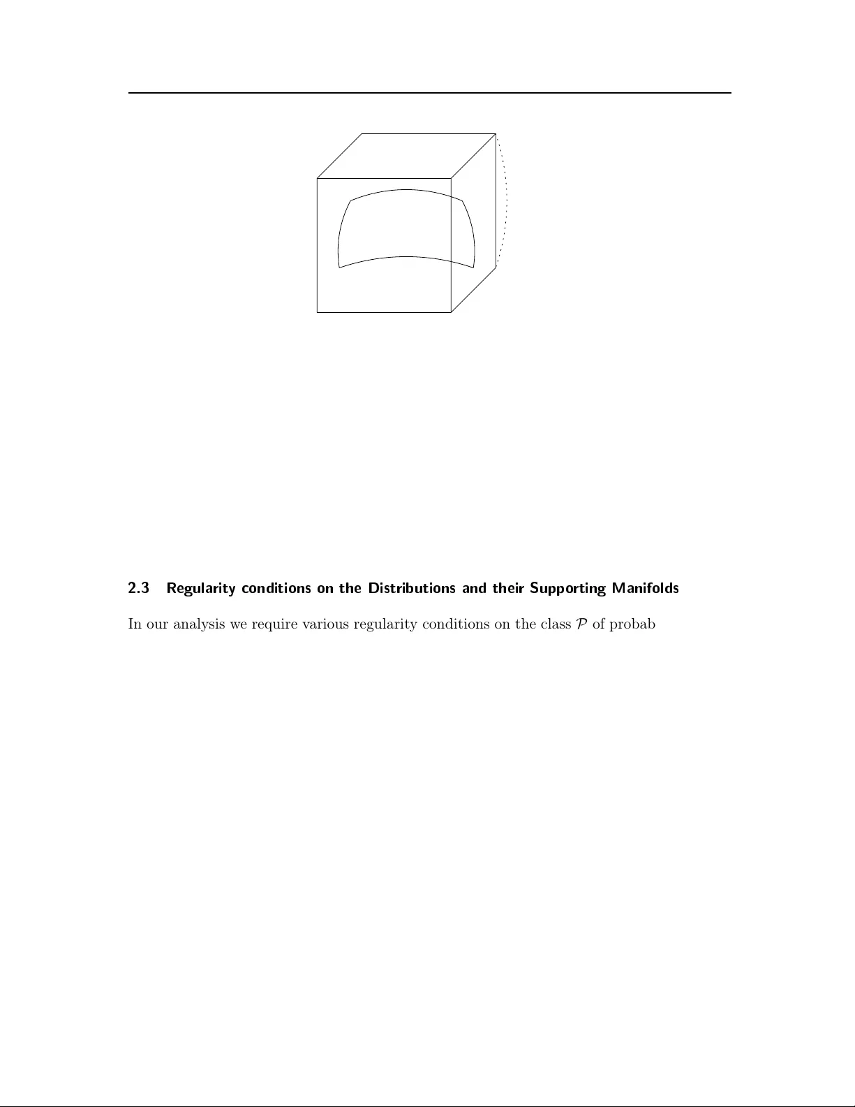
Journal of Computational Geometry jocg.org MINIMAX RA TES F OR ESTIMA TING THE DIMENSION OF A MANIF OLD Jisu Kim, ∗ A lessandr o Rinaldo, † and L arry W asserman ‡ Abstra ct. Man y algorithms in mac hine learning and computational geometry require, as input, the intrinsic dimension of the manifold that supp orts the probability distribution of the data. This parameter is rarely kno wn and therefore has to b e estimated. W e characterize the statistical diﬃculty of this problem b y deriving upp er and low er b ounds on the minimax rate for estimating the dimension. First, we consider the problem of testing the h yp othesis that the supp ort of the data-generating probabilit y distribution is a w ell-b eha ved manifold of in trinsic dimension d 1 v ersus the alternativ e that it is of dimension d 2 , with d 1 < d 2 . With an i.i.d. sample of size n , w e provide an upp er b ound on the probability of choosing the wrong dimension of O  n − ( d 2 /d 1 − 1 −  ) n  , where  is an arbitrarily small p ositiv e num b er. The pro of is based on b ounding the length of the trav eling salesman path through the data p oin ts. W e also demonstrate a low er b ound of Ω  n − (2 d 2 − 2 d 1 +  ) n  , by applying Le Cam’s lemma with a sp eciﬁc set of d 1 -dimensional probabilit y distributions. W e then extend these results to get minimax rates for estimating the dimension of w ell-b eha v ed manifolds. W e obtain an upp er bound of order O  n − ( 1 m − 1 −  ) n  and a low er b ound of order Ω  n − (2+  ) n  , where m is the em b edding dimension. 1 Intro duction Supp ose that X 1 , . . . , X n is an i.i.d. sample from a distribution P whose supp ort is an unkno wn, w ell-b eha v ed, manifold M of dimension d in R m , where 1 ≤ d ≤ m . Manifold learning refers broadly to a suite of techniques from statistics and machine learning aimed at estimating M or some of its features based on the data. Manifold learning pro cedures are widely used in high dimensional data analysis, mainly to alleviate the curse of dimensionality . Suc h algorithms map the data to a new, lo wer dimensional coordinate system [ Bellman , 1961 , Lee and V erleysen , 2007a , Hastie et al. , ∗ Carne gie Mel lon University , jisuk1@andrew.cmu.edu , supp orted b y Samsung Scholarship and partially supp orted by NSF CAREER Grant DMS 1149677. † Carne gie Mel lon University , arinaldo@cmu.edu , partially supp orted by NSF CAREER Grant DMS 1149677. ‡ Carne gie Mel lon University , larry@stat.cmu.edu 1 Journal of Computational Geometry jocg.org 2009 ], with little loss in accuracy . Manifold learning can greatly reduce the dimensionality of the data. Most manifold learning techniques require, as input, the in trinsic dimension of the manifold. How ev er, this quantit y is almost never kno wn in adv ance and therefore has to b e estimated from the data. V arious intrinsic dimension estimators hav e been prop osed and analyzed; [see, e.g., Lee and V erleysen , 2007b , Koltc hinskii , 2000 , Kégl , 2003 , Levina et al. , 2004 , Hein and Audib ert , 2005 , Raginsky and Lazebnik , 2005 , Little et al. , 2009 , 2011 , Sric haran et al. , 2010 , Rozza et al. , 2012 , Camastra and Staiano , 2016 ]. How ev er, c haracterizing the intrinsic statistical hardness of estimating the dimension remains an op en problem. The traditional w a y of measuring the diﬃcult y of a statistical problem is to b ound its minimax risk, which in the presen t setting is lo osely describ ed as the worst p ossible statistical p erformance of an optimal dimension estimator. F ormally , giv en a class of prob- abilit y distribution P , the minimax risk R n = R n ( P ) is deﬁned as R n = inf b d n sup P ∈P E P h 1( b d n 6 = d ( P )) i . (1.1) In Equation ( 1.1 ), d ( P ) is the dimension of the supp ort of P , E P denotes the exp ectation with resp ect to the distribution P , 1( · ) is the indicator function, and the inﬁmum is o ver all estimators (measurable functions of the data) b d n = b d n ( X 1 , . . . , X n ) of the dimension d ( P ) . The risk E P [1( b d n 6 = d ( P ))] of a dimension estimator b d n is the probabilit y that b d n diﬀers from the true dimension d ( P ) of the supp ort of the data generating distribution P . The minimax risk R n ( P ) , whic h is a function of b oth the sample size n and the class P , quan tiﬁes the in trinsic hardness of the dimension estimation problem, in the sense that any dimension estimator cannot ha ve a risk smaller than R n uniformly o ver every P ∈ P . The purp ose of this pap er is to obtain upp er and low er b ounds on the minimax risk R n in ( 1.1 ). W e imp ose several regularit y conditions on the set of manifolds supp orting the distribution in the class P , in order to mak e the problem analytically tractable and also to a void pathological cases, suc h as space-ﬁlling manifolds. W e ﬁrst assume that the manifold supp orting the data generating distribution P has tw o possible dimensions, d 1 and d 2 . This assumption is then relaxed to any dimension d ( P ) b et w een 1 and the embedding dimension m . Our main result is the following theorem. See Section 2 for the deﬁnition of the class P of probabilit y distributions supp orted on w ell-b eha ved manifolds in R m . Theorem 1. The minimax risk R n in ( 1.1 ) satisﬁes , a n ≤ R n ≤ b n , wher e a n = ( C (17) K I ) n min { τ − 4 ` n − 2 , 1 } n , (1.2) b n = ( C (15) K I ,K p ,K v ,m ) n max n 1 , τ − ( m 2 − m ) n g o n − n m − 1 , (1.3) and the c onstants τ ` , τ g , C (17) K I and C (15) K I ,K p ,K v ,m dep end on P and ar e deﬁne d in Se ction 5 . 2 Journal of Computational Geometry jocg.org W e now make a few remarks ab out the previous theorem. • Since the dimension d ( P ) is a discrete quan tity , the minimax rate R n in ( 1.1 ) is sup erexponential in sample size. This result seems at o dds with the exp onential rate obtained b y [ K oltchinskii , 2000 , Prop osition 2.1]. These diﬀerent rates are due to diﬀeren t mo del assumptions. In [ Koltc hinskii , 2000 ] the data generating distribution is the con volution of a probability distribution supp orted on a manifold with a noise distribution supp orted on a set of full dimension m . In contrast, here we assume that the data are generated from a probability distribution supp orted on a manifold. Under our noiseless mo del, distributions supp orted on manifolds with diﬀeren t dimension are more easily distinguishable, hence the minimax rate R n con verges to 0 faster than under the mo del with noise assumed b y [ Koltc hinskii , 2000 ]. • The key quantities that app ear in the low er b ound ( 1.2 ) and the upp er b ound ( 1.3 ) are the global reac h τ g and the lo cal reach τ ` of the manifold, whic h are deﬁned in Section 2 . These reach parameters can b e roughly though t as the inv erse of the usual notion of curv ature [see, e.g. F ederer , 1959 ], and they aﬀect the p erformance of an y dimension estimator: a manifold with lo w reach may app ear more space-ﬁlling than a manifold of the same dimension but with higher reac h, thus making the task of resolving the dimension harder. Indeed, our analysis shows formally that the minimax risk R n in ( 1.1 ) decreases in the v alues of the reaches. Giv en their crucial role, w e ha ve attempted to make the dep endence of the minimax risk R n on b oth τ g and τ ` as explicit as p ossible. • There is a gap b et w een the low er b ound ( 1.2 ) and the upp er b ound ( 1.3 ). Nonetheless, as far as w e are aw are, these are the most precise b ounds on R n that are a v ailable. This pap er is organized as follo ws. In Section 2 , we formulate and discuss regularity conditions on distributions and their supp orting manifolds. In Section 3 , we pro vide an upp er b ound on the minimax rate by considering the trav eling salesman path through the p oin ts. In Section 4 , w e derive a low er b ound on the minimax rate b y applying Le Cam’s lemma with a sp eciﬁc set of d 1 -dimensional and d 2 -dimensional probabilit y distributions. In Section 5 , we extend our upp er b ound and low er b ound for the case where the in trinsic dimension v aries from 1 to m . 2 Denitions and Re gula rit y Conditions In this section, we deﬁne the set P of probabilit y distributions that we consider in b ound- ing the minimax risk R n in ( 1.1 ). Suc h distributions are supp orted on manifolds whose dimension d is b et w een 1 and m , where m is the dimension of the em b edding space. In 3 Journal of Computational Geometry jocg.org particular, w e require that the supp orting manifolds hav e a uniform low er b ound on their reac h parameters τ g and τ l . The resulting class of distributions is denoted by P = m [ d =1 P d τ g ,τ ` ,K I ,K v ,K p . (2.1) In the rest of this section, w e will mak e the deﬁnition P d τ g ,τ ` ,K I ,K v ,K p precise. Readers who are not interested in the details may skip the rest of the section. All the pro ofs for this section are in Section A . 2.1 Notation and Basic Denitions F or the reader’s conv enience, we provide a list of the notation used throughout the pap er in T able 1 . W e no w brieﬂy review some notations from diﬀerential geometry . F or a more de- tailed treatment, we refer the reader to standard textb ooks on this topic [see, e.g., Lee , 2000 , 2003 , P etersen , 2006 , do Carmo , 1992 ]. A top ological manifold of dimension d is a top ological space M and a family of homeomorphisms ϕ α : U α ⊂ R d → V α ⊂ M from an op en subset of R d to an op en subset of M such that S α ϕ α ( U α ) = M . A top ological space M is considered to b e a d -dimensional manifold if there exists a family of homeomorphisms ϕ α : U α ⊂ R d → V α ⊂ M suc h that ( M , { ϕ α } α ) is a manifold. If M is a d -dimensional manifold, suc h d is unique and is called the dimension of a manifold. If, for any pair α , β , with ϕ α ( U α ) ∩ ϕ β ( U β ) 6 = ∅ , ϕ − 1 β ◦ ϕ α : U α ∩ U β → U α ∩ U β is C k , then M is a C k -manifold. W e assume that the top ological manifold M is em b edded in R m , i.e. M ⊂ R m , and the metric is inherited from the metric of R m . F or a top ological manifold M ⊂ R m and for an y p, q ∈ M , a path joining p to q is a map γ : [ a, b ] → M for some a, b ∈ R such that γ ( a ) = p , γ ( b ) = q . The length of the curv e γ is deﬁned as Leng th ( γ ) = ´ b a || γ 0 ( t ) || 2 dt . A top ological manifold M is equipped with the distance dist M : M × M → R as dist M ( p, q ) = inf γ : path joining p and q Leng th ( γ ) . A path γ : [ a, b ] → M is a geo desic if for all t, t 0 ∈ [ a, b ] , dist M ( γ ( t ) , γ ( t 0 )) = | t − t 0 | . Let T p M denote the tangen t space to M at p . Giv en p ∈ M , there exist a set 0 ∈ E ⊂ T p ( M ) and a mapping exp p : E ⊂ T p M → M suc h that t → exp p ( tv ) , t ∈ ( − 1 , 1) , is the unique geo desic of M which, at t = 0 , passes through p with velocity v , for all v ∈ E . The map exp p : E ⊂ T p M → M is called the exp onen tial map on p . One of the k ey conditions that we imp ose in Section 2.3 is ab out the reac h. Deﬁnition 1. F or a compact d -dimensional top ological manifold M ⊂ R m (with b ound- ary), the r e ach of M , τ ( M ) , is deﬁned as the largest v alue of r > 0 such that each x ∈ R m 4 Journal of Computational Geometry jocg.org Notation Deﬁnition 1( · ) indicator function. d , d 1 , d 2 dimension of a manifold. b d n dimension estimator. dist A ( · , · ) distance function on the set A . dist A, ||·|| ( · , · ) distance function on the set A induced b y the norm || · || . exp p ( · ) exp onen tial map on p oin t p ∈ M . ` ( · , · ) loss function. n size of the sample. m dimension of the em b edding space. p , q p oints on the manifold M . v ol A ( · ) volume function of A . B A ( x, r ) op en ball with center x and radius r , { y ∈ A : dist A ( y , x ) < r } . C a 1 ,...,a k constan t that dep ends only on a 1 , . . . , a k . I cub e [ − K I , K I ] m . K I , K v , K p ﬁxed constan ts for regular conditions; see Deﬁnition 2 . M manifold. P data generating probabilit y distribution. R n minimax risk inf b d n sup P ∈P E P h 1  b d n 6 = d ( P ) i ; see ( 1.1 ), ( 2.5 ), and ( 2.6 ). S n p erm utation group on { 1 , . . . , n } . T subset of I n ⊂ ( R d ) n , used in Section 4 . T p M tangen t space of a manifold M at p . X 1 , . . . , X n sample p oin ts. M set of manifolds; see Deﬁnition 2 . P set of distributions; see Deﬁnition 2 . γ path on a manifold M . π A ( · ) pro jection function onto a closed set A . σ permutation. τ ( M ) reac h of a manifold M ; see Deﬁnition 1 and Lemma 2 . τ g lo wer b ound for global reac h; see Deﬁnition 2 . τ ` lo wer b ound for lo cal reach; see Deﬁnition 2 . ω d v olume of the unit ball in R d , π d 2 Γ ( d 2 +1 ) . Π n 1 : n 2 co ordinate pro jection map: Π n 1 : n 2 ( x 1 , . . . , x d ) = ( x n 1 , . . . , x n d ) . T able 1: T able of notations and deﬁnitions. with dist R m ( x, M ) < r has a unique pro jection π M ( x ) on M , i.e. τ ( M ) := sup n r : ∀ x ∈ R m with dist R m ( x, M ) < r, ∃ ! π M ( x ) ∈ M s.t. || x − π M ( x ) || 2 = inf y ∈ M || x − y || 2 o . (2.2) 5 Journal of Computational Geometry jocg.org π M ( x ) x τ ( M ) M (a) reac h τ ( M ) in Deﬁnition 1 . τ ( M ) τ ( M ) M x (b) reac h τ ( M ) in Lemma 2 . Figure 2.1: F or a manifold M , there are several equiv alent deﬁnitions for reach τ ( M ) in Deﬁnition 1 . (a) The reac h τ ( M ) is the supremum v alue of r such that for all x ∈ R m with dist R m ( x, M ) < r has unique pro jection π M ( x ) to M , as in ( 2.2 ). (b) The reach τ ( M ) is the maxim um radius of a ball that you can roll ov er the manifold M , as in ( 2.3 ). See [ F ederer , 1959 ] for further details. The reach τ ( M ) can b e also considered as one kind of curv ature, and can b e understo o d as an inv erse of other usual curv atures. See Figure 2.1(a) for the illustration of Deﬁnition 1 . There are sev eral equiv alent wa ys to deﬁne the reach τ ( M ) in ( 2.2 ) for the manifold M . The reach τ ( M ) is the maximum radius of a ball that can b e rolled freely o v er the manifold M , as in Lemma 2 . See Figure 2.1(b) for the illustration of Lemma 2 . Lemma 2. F or a manifold M ⊂ R m , τ ( M ) = sup  r : ∀ x ∈ M , ∀ y ∈ R m with y − x ⊥ T x M and || y − x || 2 = r , B R m ( y , r ) ∩ M = ∅  . (2.3) Pr o of of L emma 2 . [See F ederer , 1959 , Theorem 4.18]. 2.2 Minimax Theo ry The minimax rate is the risk of an estimator that p erforms b est in the worst case, as a function of the sample size [see, e.g. T sybako v , 2008 ]. Let P b e a collection of probability distributions ov er the same sample space X and let θ : P → Θ b e a function ov er P taking 6 Journal of Computational Geometry jocg.org v alues in some space Θ , the parameter space. W e can think of θ ( P ) as the feature of interest of the probability distribution P , such as its mean, or, as in our case, the dimension of its supp ort. F or the ﬁxed sample size n , supp ose X = ( X 1 , . . . , X n ) is an i.i.d. (indep enden t and identically distributed) sample drawn from a ﬁxed probability distribution P ∈ P . Th us X takes v alues in the n -fold pro duct space X n = X × · · · × X and is distributed as P ( n ) , the n -fold pro duct measure. An estimator b θ n : R n → Θ is any measurable function that maps the observ ation X in to the parameter space Θ . Let ` : Θ × Θ → R b e a loss function, a non-negative b ounded function that measures ho w diﬀeren t t wo parameters are. Then for a ﬁxed estimator b θ n and a ﬁxed distribution P , the risk of b θ n is deﬁned as E P ( n ) h `  b θ n ( X ) , θ ( P ) i . Then for a ﬁxed estimator b θ n , its maxim um risk is the suprem um of its risk ov er every distribution P ∈ P , that is, sup P ∈P E P ( n ) h `  b θ n ( X ) , θ ( P ) i . (2.4) The minimax risk asso ciated with P , θ , ` and n is the maximal risk of any estimator that p erforms the b est under the worst p ossible choice of P . F ormally , the minimax risk is R n = inf b θ n sup P ∈P E P ( n ) h `  b θ n ( X ) , θ ( P ) i . (2.5) The minimax risk R n in ( 2.5 ) is often viewed as a function of the sample size n , in which case an y p ositiv e sequence ψ n suc h that lim n →∞ R n /ψ n remains b ounded aw a y from 0 and ∞ is called a minimax r ate. Notice that minimax rates are unique up to constants and lo wer order terms. T o deﬁne a meaningful minimax risk, it is essen tial to hav e some constraint on the set of distributions P in ( 2.4 ) and ( 2.5 ). If P is to o large, then the minimax rate R n in ( 2.5 ) will not conv erge to 0 as n go es to ∞ : this means that the problem is statistically ill-p osed. If P is to o small, the minimax estimator dep ends to o muc h on the sp eciﬁc distributions in P and is not a useful measure of a statistical diﬃculty . Determining the v alue of the minimax risk R n in ( 2.5 ) for a given problem requires t wo separate calculations: an upp er b ound on R n and a lo wer b ound. In order to deriv e an upp er b ound, one analyzes the asymptotic risk of a sp eciﬁc estimator b θ n . Low er b ounds are instead usually computed by measuring the diﬃculty of a m ultiple hypothesis testing problem that entails identifying ﬁnitely many distributions in P that are maximally diﬃcult to discriminate [see, e.g. T sybako v , 2008 , Section 2.2]. F or the dimension estimation problem, we obtain an upp er b ound on R n b y analyz- ing the p erformance of an estimator based on the length of the trav eling salesman problem, as describ ed in Section 3 . On the other hand, the calculation of the low er b ound presents 7 Journal of Computational Geometry jocg.org 2 K I M Figure 2.2: A manifold M is assumed to b e con tained inside the cub e I = [ − K I , K I ] m , for some K I > 0 . See Deﬁnition 2 . non-trivial technical diﬃculties, b ecause probability distributions supp orted on manifolds of diﬀeren t dimensions are singular with resp ect to each other, and therefore trivially discrim- inable. In order to ov ercome suc h an issue, w e resort to constructing mixtures of mutually singular distributions. W e detail this construction in Section 4 . There is a gap b et ween the lo wer and upp er b ounds we derive on the minimax risk, as it is often the case in such calculations. Nonetheless, the deriv ation of the b ounds is of use in understanding the diﬃcult y of the dimension estimation problem. 2.3 Regula rit y conditions on the Distributions and their Supp o rting Manifolds In our analysis we require v arious regularit y conditions on the class P of probability distri- butions app earing in the minimax risk ( 1.1 ). Most of these conditions are of a geometric nature and concern the prop erties of the manifolds supp orting the probability distributions in P . Altogether, our assumptions rule out manifolds that are so complicated to make the dimension estimation problem unsolv able and, therefore, guarantee that the minimax risk R n in ( 2.5 ) conv erges to 0 as n go es to ∞ . Such regularit y assumptions are quite mild, and in fact allo w for virtually all types of manifolds usually encountered in manifold learning problems. Our ﬁrst assumption is that the probability distributions in P are supp orted o v er manifold con tained inside a compact set, whic h, without loss of generality , we take to b e the cub e I := [ − K I , K I ] m , for some K I > 0 . See Figure 2.2 . Second, to exclude manifolds that are arbitrarily complicated in the sense of having un b ounded curv atures or of being nearly self in tersecting, we assume that the reac h is uniformly b ounded from b elo w. More precisely , we will constrain b oth the global reach and the lo cal reach as follows. Fix τ g , τ ` ∈ (0 , ∞ ] with τ g ≤ τ ` . The global reach condition for a 8 Journal of Computational Geometry jocg.org τ g τ g M x (a) global reach condition ≤ τ ` y π U x ( y ) x U x (b) lo cal reach condition Figure 2.3: A manifold M with (a) glob al r e ach at least τ g , or (b) lo c al r e ach at least τ ` . See Deﬁnition 2 . manifold M is that the usual reach τ ( M ) in ( 2.2 ) is low er b ounded b y τ g as in Figure 2.3(a) , and the lo cal reac h condition is that M can b e cov ered b y small patc hes whose reac hes are lo wer b ounded b y τ ` , as in Figure 2.3(b) . (See Deﬁnition 2 b elo w for more details.) Third, w e assume that the data are generated from a distribution P supp orted on a manifold M having a density with resp ect to the (restriction of the) Hausdorﬀ measure on M b ounded from ab o v e b y some p ositiv e constant K p . F or manifolds without b oundary , the ab o ve conditions suﬃce for our analysis. How- ev er, to deal with manifolds with b oundary , w e need further assumptions, namely lo cal geo desic completeness and essential dimension. A manifold M is said to b e complete if an y geo desic can b e extended arbitrarily farther, i.e. for any geo desic path γ : [ a, b ] → M , there exists a geo desic ˜ γ : R → M that satisﬁes ˜ γ | [ a,b ] = γ . [see, e.g., Lee , 2000 , 2003 , Petersen , 2006 , do Carmo , 1992 ]. Accordingly , we deﬁne a manifold M to b e lo cally (geo desically) complete, if any tw o p oint s inside a geo desic ball of small enough radius in the interior of M can b e joined b y a geo desic whose image also lies on the in terior of M . Fifth, w e assume the manifold M is of essential dimension d , in v olume sense. If w e ﬁx any p oin t p in the d -dimensional manifold M , then the volume of a ball of radius r grows in order of r d when r is small. By extending this, ﬁx K v ∈ (0 , 2 − m ] , and w e sa y that the manifold M is of essential volume dimension d , if the volume of a geo desic ball of radius r around any p oint in M is lo wer b ounded b y K v r d ω d , for some p ositiv e constant K v and all r small enough. 9 Journal of Computational Geometry jocg.org W e are now ready to formally deﬁne the class P of probability distributions that w e will consider in our analysis of the minimax problem ( 1.1 ). Deﬁnition 2. Fix τ g , τ ` ∈ (0 , ∞ ] , K I ∈ [1 , ∞ ) , K v ∈ (0 , 2 − m ] , with τ g ≤ τ ` . Let M d τ g ,τ ` ,K I ,K v b e the set of compact d -dimensional manifolds M suc h that: (1) M ⊂ I := [ − K I , K I ] m ⊂ R m ; (2) M is of glob al r e ach at least τ g , i.e. τ ( M ) ≥ τ g , and M is of lo c al r e ach at least τ ` , i.e. for all p ∈ M , there exists a neighborho o d U p in M suc h that τ ( U p ) ≥ τ ` ; (3) M is lo c al ly (ge o desic al ly) c omplete (with resp ect to τ g ): for all p ∈ int( M ) and for all q 1 , q 2 ∈ B M ( p, 2 √ 3 τ g ) , there exists a geo desic γ joining q 1 and q 2 whose image lies on intM ; (4) M is of essential volume dimension d (with resp ect to K v and τ g ): if for all p ∈ M and for all r ≤ √ 3 τ g , v ol M ( B M ( p, r )) ≥ K v r d ω d . Let P = P d τ g ,τ ` ,K I ,K v ,K p b e the set of Borel probabilit y distributions P such that: (5) P is supp orted on a d -dimensional manifold M ∈ M d τ g ,τ ` ,K I ,K v ; (6) P is absolutely contin uous with resp ect to the restriction v ol M of the d -dimensional Hausdorﬀ measure on the supp orting manifold M and such that sup x ∈ M dP dv ol M ( x ) ≤ K p . F or every P ∈ P d τ g ,τ ` ,K I ,K v ,K p , denote the dimension of its distribution as d ( P ) . R emark 1 . F or manifolds without b oundary , the lo cal completeness condition and the es- sen tial volume dimension condition in Deﬁnition 2 alwa ys hold. The Hopf Rinow Theorem [see, e.g. Petersen , 2006 , Theorem 16] implies that any compact closed manifold without b oundary is geo desic complete, whic h implies it is lo cally complete in the sense of (3) in Def- inition 2 . Also, [ Niyogi et al. , 2008 , Lemma 5.3] implies that, for a d -dimensional manifold M and all 0 < r ≤ 2 τ ( M ) , v ol M ( B M ( p, r )) ≥ r d 1 −  r 2 τ ( M )  2 ! d 2 ω d , for all p ∈ M . Hence, when, for ﬁxed τ g > 0 , a d -dimensional manifold M (without b oundary) satisﬁes τ ( M ) ≥ τ g , then for any 0 < r ≤ √ 3 τ g , v ol M ( B M ( p, r )) ≥ 2 − d r d ω d , so the essen tial volume dimension condition is satisﬁed. 10 Journal of Computational Geometry jocg.org R emark 2 . The notion of the lo cal reach τ ` in Deﬁnition 2 is less standard than the global reac h τ g , whic h is the usual deﬁnition of the reac h in [see, e.g. F ederer , 1959 ]. The lo cal reac h condition is only used in getting the low er b ound of the minimax rate R n in Section 4 , while the global reach condition is used in b oth Section 3 and Section 4 . In fact, the reac h of the manifold is determined either by a b ottleneck structure or an area of high curv ature, as in [ Aamari et al. , 2017 , Theorem 3.4]. And the global reach condition is imp osing regularities on b oth cases, while the lo cal reach condition is imp osing regularities only on the latter case, i.e. on the lo cal curv ature. Setting the lo cal reach τ ` equal to the global reac h τ g reduces to the mo del that has conditions only on the usual reac h. The regularit y conditions in Deﬁnition 2 imply further constrain ts on both the distributions in P and their supp orting manifolds, in Lemma 3 , 4 , and 5 . Such prop erties are exploited in Section 3 and 4 . The pro ofs for Lemma 3 , 4 , and 5 are in App endix A . Lemma 3. Fix τ g ∈ (0 , ∞ ] , and let M b e a d -dimensional manifold with glob al r e ach ≥ τ g . F or r ∈ (0 , τ g ) , let M r := { x ∈ R m : dist R m , ( x, M ) < r } b e an r -neighb orho o d of M in R m . Then, the volume of M is upp er b ounde d as v ol M ( M ) ≤ m ! d ! r d − m v ol R m ( M r ) . F urther, ﬁx τ ` ∈ (0 , ∞ ] , K I ∈ [1 , ∞ ) , K v ∈ (0 , 2 − m ] , with τ g ≤ τ ` , and supp ose M ∈ M d τ g ,τ ` ,K I ,K v . Then the volume of M is upp er b ounde d as v ol M ( M ) ≤ C (3) K I ,m max n 1 , τ d − m g o , wher e C (3) K I ,m is a c onstant dep ending only on K I and m . Lemma 4. Fix τ g , τ ` ∈ (0 , ∞ ] , K I ∈ [1 , ∞ ) , K v ∈ (0 , 2 − m ] , with τ g ≤ τ ` . L et M ∈ M d τ g ,τ ` ,K I ,K v and r ∈ (0 , 2 √ 3 τ g ] . Then M c an b e c over e d by N r adius r b al ls B M ( p 1 , r ) , . . . , B M ( p N , r ) , with N ≤  2 d v ol ( M ) K v r d ω d  . Lemma 5. Fix τ g , τ ` ∈ (0 , ∞ ] , K I ∈ [1 , ∞ ) , K v ∈ (0 , 2 − m ] , with τ g ≤ τ ` . L et M ∈ M d τ g ,τ ` ,K I ,K v and let exp p k : E k ⊂ R m → M b e an exp onential map, wher e E k is the domain of the exp onential map exp p k and T p k M is identiﬁe d with R d . F or al l v , w ∈ E k , let R k := max {|| v || , || w ||} . Then k exp p k ( v ) − exp p k ( w ) k R m ≤ sinh( √ 2 R k /τ ` ) √ 2 R k /τ ` k v − w k R d . 11 Journal of Computational Geometry jocg.org Under these regularit y conditions, the minimax risk R n is deﬁned as R n = inf b d n sup P ∈P E P ( n ) h 1  b d n ( X ) 6 = d ( P ) i , (2.6) where in Section 3 and 4 w e ﬁx d 1 , d 2 ∈ N with 1 ≤ d 1 < d 2 ≤ m and deﬁne P = P d 1 τ g ,τ ` ,K I ,K v ,K p [ P d 2 τ g ,τ ` ,K I ,K v ,K p , (2.7) and in Section 5 w e set instead P = m [ d =1 P d τ g ,τ ` ,K I ,K v ,K p . (2.8) In ( 2.6 ), b d n is any dimension estimator based on data X = ( X 1 , . . . , X n ) , and the loss function ` ( · , · ) is 0 − 1 loss, so for all x, y ∈ R , ` ( x, y ) = 1( x 6 = y ) . 3 Upp e r Bound fo r Cho osin g Bet w een Tw o Dimensions In this section w e provide an upp er b ound on the minimax rate R n in ( 2.6 ) when d ( P ) can only take tw o kno wn v alues. Fix d 1 , d 2 ∈ N with 1 ≤ d 1 < d 2 ≤ m , and assume that the data are generated from a distribution P ∈ P such that either d ( P ) = d 1 or d ( P ) = d 2 as in ( 2.7 ). In this case, the minimax risk quan tiﬁes the statistical hardness of the hypothesis testing problem of deciding whether the data originate from a d 1 or d 2 -dimensional distribution. In Section 5 we will relax this assumption and allow for the in trinsic dimension d ( P ) to b e an y integer b etw een 1 and m as in ( 2.8 ). All the pro ofs for this section are in Section B . Our strategy to deriv e an upp er b ound on R n is to choose a particular estimator b d n and then derive a uniform upp er b ound on its risk ov er the class P in ( 2.7 ), i.e. an upp er b ound for the quantit y sup P ∈P E P ( n ) h 1  b d n ( X ) 6 = d ( P ) i , (3.1) where P ( n ) denotes the n -fold pro duct of P . This will in turn yield an upp er b ound on the minimax risk R n , since R n = inf b d n sup P ∈P E P ( n ) h 1  b d n ( X ) 6 = d ( P ) i ≤ sup P ∈P E P ( n ) h 1  b d n ( X ) 6 = d ( P ) i . (3.2) Naturally , choosing an appropriate estimator is critical to get a sharp b ound. In Section 3.1 , we deﬁne our dimension estimator b d n and analyze its risk. F rom that analysis, w e deriv e an upp er b ound on the minimax risk R n in ( 2.6 ) in Section 3.2 . 12 Journal of Computational Geometry jocg.org 3.1 Dimension Estimato r and its Analysi s Our dimension estimator b d n is based on the d 1 -squared length of the TSP (T ra v eling Sales- man P ath) generated b y the data. The d 1 -squared length of the TSP generated b y the data is the minimal d 1 -squared length of all p ossible paths passing through each sample p oin t X i once, whic h is min σ ∈ S n ( n − 1 X i =1 k X σ ( i +1) − X σ ( i ) k d 1 R m ) . (3.3) Then, b d n = d 1 if and only if the d 1 -squared length of the TSP is b elo w a certain threshold; that is b d n ( X ) :=      d 1 , if min σ ∈ S n  n − 1 P i =1 k X σ ( i +1) − X σ ( i ) k d 1 R m  ≤ C (7) K I ,K v ,m max  1 , τ d 1 − m g  , d 2 , otherwise. (3.4) where C (7) K I ,K v ,m is a constan t to b e deﬁned later. W e b egin our analysis of the estimator b d n with Lemma 6 , whic h shows that b d n mak es an error with probability of order O  n −  d 2 d 1 − 1  n  if the correct dimension is d 2 . Sp eciﬁcally , w e demonstrate that, for an y p ositiv e v alue L , the d 1 -squared length of a piecewise linear path from X 1 to X n , n − 1 P i =1 k X i +1 − X i k d 1 R m , is upp er b ounded b y L with a v ery small probability of order O  n −  d 2 d 1 − 1  n  , as in ( 3.5 ). Hence the d 1 -squared length of the path is not lik ely to b e b ounded b y an y such threshold L . Lemma 6. Fix τ g , τ ` ∈ (0 , ∞ ] , K I ∈ [1 , ∞ ) , K v ∈ (0 , 2 − m ] , K p ∈ [(2 K I ) m , ∞ ) , d 1 , d 2 ∈ N , with τ g ≤ τ ` and 1 ≤ d 1 < d 2 ≤ m . L et X 1 , . . . , X n ∼ P ∈ P d 2 τ g ,τ ` ,K I ,K v ,K p . Then for al l L > 0 , P ( n ) " n − 1 X i =1 k X i +1 − X i k d 1 R m ≤ L # ≤  C (6) K I ,K p ,m  n − 1 L d 2 d 1 ( n − 1) max n 1 , τ ( d 2 − m )( n − 1) g o ( n − 1)  d 2 d 1 − 1  ( n − 1) ( n − 1)! , (3.5) wher e C (6) K I ,K p ,m is a c onstant dep ending only on K I , K p , and m . Pr o of of L emma 6 . in App endix B . Next, Lemma 7 sho ws that the estimator b d n in ( 3.4 ) is alwa ys correct when the in trinsic dimension is d 1 , as in ( 3.6 ). Sp eciﬁcally , the d 1 -squared length of the TSP path 13 Journal of Computational Geometry jocg.org X σ (1) X σ (2) X σ (3) X σ ( n − 1) X σ ( n ) . . . Y 1 Y 2 Y n − 1 P Y i ≤ v ol M ( M ) M X σ ( n − 2) Y n − 2 Figure 3.1: When the manifold is a curv e, the length of the TSP path min σ ∈ S n  n − 1 P i =1 k X σ ( i +1) − X σ ( i ) k R m  in ( 3.3 ) is upp er b ounded b y the length of the curve v ol M ( M ) . in ( 3.3 ) is b ounded by some p ositiv e threshold C (7) K I ,K v ,m max  1 , τ d 1 − m g  . W e take note that, when d 1 = 1 , Lemma 7 is straigh tforward: the length of the TSP path in ( 3.3 ) is upp er b ounded b y the length of curve v ol M ( M ) , as in Figure 3.1 . This fact, com bined with Lemma 3 , which sho ws that v ol M ( M ) ≤ C (3) K I ,m max  1 , τ 1 − m g  , yields the result. In particular, the constan t C (7) K I ,K v ,m can b e set as C (7) K I ,K v ,m = C (3) K I ,m . When d 1 > 1 , Lemma 7 is prov ed using Lemma 3 , 4 and 5 , along with the Hölder con tinuit y of a d 1 -dimensional space-ﬁlling curv e [ Steele , 1997 , Buchin , 2008 ]. Lemma 7. Fix τ g , τ ` ∈ (0 , ∞ ] , K I ∈ [1 , ∞ ) , K v ∈ (0 , 2 − m ] , d 1 ∈ N , with τ g ≤ τ ` . L et M ∈ M d 1 τ g ,τ ` ,K p ,K v and X 1 , . . . , X n ∈ M . Then min σ ∈ S n n − 1 X i =1 k X σ ( i +1) − X σ ( i ) k d 1 R m ≤ C (7) K I ,K v ,m max n 1 , τ d 1 − m g o , (3.6) wher e C (7) K I ,K v ,m is a c onstant dep ending only on K I , K v , and m . Pr o of of L emma 7 . in App endix B . Prop osition 8 b elow is the main result of this subsection and follo ws directly from Lemma 6 and Lemma 7 ab ov e. Indeed, when the intrinsic dimension is d 2 , the risk of our estimator b d n , is of order O  n −  d 2 d 1 − 1  n  b y Lemma 6 and the union b ound. On the other hand, when the intrinsic dimension is d 1 , the risk of our estimator b d n is 0 , b ecause of Lemma 7 . 14 Journal of Computational Geometry jocg.org Prop osition 8. Fix τ g , τ ` ∈ (0 , ∞ ] , K I ∈ [1 , ∞ ) , K v ∈ (0 , 2 − m ] , K p ∈ [(2 K I ) m , ∞ ) , d 1 , d 2 ∈ N , with τ g ≤ τ ` and 1 ≤ d 1 < d 2 ≤ m . L et b d n b e in ( 3.4 ) . Then either for d = d 1 or d = d 2 , sup P ∈P d τ g ,τ ` ,K I ,K v ,K p E P ( n ) h `  b d n , d ( P ) i ≤ 1( d = d 2 )  C (8) K I ,K p ,K v ,m  n max ( 1 , τ −  d 2 d 1 m + m − 2 d 2  n g ) n −  d 2 d 1 − 1  n , wher e C (8) K I ,K p ,K v ,m ∈ (0 , ∞ ) is a c onstant dep ending only on K I , K p , K v , and m . Pr o of of Pr op osition 8 . in App endix B . As describ ed so far, the con v ergence analysis of our dimension estimator is probable. This is enough for our purp ose, which is to quan tify the statistical diﬃculties, in particular the minimax rate, of the dimension estimation problem. Ho wev er, our b d n in ( 3.4 ) is not completely data-driv en but dep ends on the mo del parameters τ g , K I , and K v . Hence the mo del on which our con v ergence analysis is v alid dep ends on the mo del parameters. When it comes to applying our dimension estimator b d n to real data, w e need to estimate the constan t C (7) K I ,K v ,m . Pro ofs of Lemma 6 and 7 suggest that ov erestimating C (7) K I ,K v ,m b y some constan t factor do esn’t deteriorate the conv ergence rate, so the constants C (7) K I ,K v ,m and τ g can b e replaced by an y consisten t estimators. Still, we hav e the diﬃculty of tuning the constant C (7) K I ,K v ,m and τ g . Also, the constant C (7) K I ,K v ,m is tuned to work for the worst case, so the practical p erformance of our dimension estimator is questionable. 3.2 Minimax Upp er Bound As noted at the b eginning of Section 3 , the maximum risk of our estimator b d n in ( 3.1 ) serv es as an upp er b ound on the minimax risk R n in ( 2.6 ). Since we assume that the intrinsic dimension is either d 1 or d 2 , Prop osition 8 yields that the maximum risk of our estimator b d n is of order O  n −  d 2 d 1 − 1  n  . This also serves as an upp er b ound of the minimax risk R n , as in Prop osition 9 . Prop osition 9. Fix τ g , τ ` ∈ (0 , ∞ ] , K I ∈ [1 , ∞ ) , K v ∈ (0 , 2 − m ] , K p ∈ [(2 K I ) m , ∞ ) , d 1 , d 2 ∈ N , with τ g ≤ τ ` and 1 ≤ d 1 < d 2 ≤ m . Then inf b d n sup P ∈P 1 ∪P 2 E P ( n ) h `  b d n , d ( P ) i ≤  C (8) K I ,K p ,K v ,m  n max ( 1 , τ −  d 2 d 1 m + m − 2 d 2  n g ) n −  d 2 d 1 − 1  n , 15 Journal of Computational Geometry jocg.org wher e C (8) K I ,K p ,K v ,m is fr om Pr op osition 8 and P 1 = P d 1 τ g ,τ ` ,K I ,K v ,K p , P 2 = P d 2 τ g ,τ ` ,K I ,K v ,K p . Pr o of of Pr op osition 9 . in App endix B . 4 Lo w er Bound fo r Cho osing B et w een Tw o Dimensions The goal of this section is to deriv e a lo wer b ound for the minimax rate R n . As in Section 3 , w e ﬁx d 1 , d 2 ∈ N with 1 ≤ d 1 < d 2 ≤ m , and assume that the in trinsic dimension of data is either d 1 or d 2 as in ( 2.7 ). This assumption is relaxed in Section 5 . All the pro ofs for this section are in Section C . Our strategy is to ﬁnd a subset T ⊂ I n ⊂ ( R d ) n and t wo sets of distributions P d 1 1 and P d 2 2 with dimensions d 1 and d 2 , such that P d 1 1 and P d 2 2 satisfy the regularity conditions in Deﬁnition 2 , and whenever the sample X = ( X 1 , . . . , X n ) lies on T , one cannot easily distinguish whether the underlying distribution is from P d 1 1 or P d 2 2 . After constructing T , P d 1 1 and P d 2 2 , we derive the low er b ound using the follo wing result, kno wn as Le Cam’s lemma. Lemma 10. (Le Cam’s Lemma) L et P b e a set of pr ob ability me asur es on (Ω , F ) , and P 1 , P 2 ⊂ P b e such that for al l P ∈ P i , θ ( P ) = θ i for i = 1 , 2 . F or any Q i ∈ co ( P i ) , wher e co ( P i ) is the c onvex hul l of P i , let q i b e the density of Q i with r esp e ct to a me asur e ν . Then inf b θ sup P ∈P E P [ ` ( b θ , θ ( P ))] ≥ ` ( θ 1 , θ 2 ) 2 ˆ [ q 1 ( x ) ∧ q 2 ( x )] dν ( x ) . (4.1) Pr o of of L emma 10 . [See Y u , 1997 , Chapter 29.2, Lemma 1]. In ab o v e Le Cam’s lemma, considering the con vex hull of distributions co ( P i ) is critical for getting the nontrivial low er b ound. Supp ose we are using the basic v ersion of Le Cam’s lemma where the conv ex h ull is not considered, i.e. Q i ∈ P i . Then for tw o distributions Q 1 and Q 2 resp ectiv ely from our d 1 and d 2 dimensional mo del P d 1 τ g ,τ l ,K I ,K v ,K p and P d 2 τ g ,τ l ,K I ,K v ,K p , Q 1 and Q 2 are singular to each other; i.e. q 1 ( x ) ∧ q 2 ( x ) = 0 for all x . Hence no matter whic h subset P 1 and P 2 w e c ho ose with d ( P 1 ) = d 1 and d ( P 2 ) = d 2 , the lo wer b ound in ( 4.1 ) will b e alwa ys 0 . This trivial b ound can b e improv ed by considering the con vex hull of distributions co ( P i ) in Le Cam’s lemma. Our construction for T , P d 1 1 , and P d 2 2 is based on mimic king a space-ﬁlling curv e. In tuitively , this gives the lo w er bound since it is diﬃcult to diﬀeren tiate a space-ﬁlling curv e 16 Journal of Computational Geometry jocg.org and a higher dimensional cub e. In detail, w e set P d 1 1 = { distributions supp orted on a space-ﬁlling-curv e like d 1 -dimensional manifold } , (4.2) and P d 2 2 = { uniform distributions on [ − K I , K I ] d 2 } . (4.3) T o apply Le Cam’s lemma, we construct a set T ⊂ I n so that, whenever X = ( X 1 , . . . , X n ) ∈ T , we cannot distinguish whether X is from P d 1 1 in ( 4.2 ) or P d 2 1 in ( 4.3 ). Then, for an appropriately chosen distribution Q 1 in the conv ex hull of P d 1 1 with density q 1 with resp ect to Leb esgue measure λ on the cub e [ − K I , K I ] d 2 , and a densit y q 2 from the class P d 2 2 , ´ T [ q 1 ( x ) ∧ q 2 ( x )] dλ ( x ) is a low er b ound on the minimax rate R n in ( 2.6 ). Indeed, from Le Cam’s Lemma 10 , w e hav e that inf b θ sup P ∈P E P [ ` ( b θ , θ ( P ))] ≥ 1 2 ˆ [ q 1 ( x ) ∧ q 2 ( x )] dλ ( x ) ≥ 1 2 ˆ T [ q 1 ( x ) ∧ q 2 ( x )] dλ ( x ) . (4.4) F or constructing the class P d 1 1 in ( 4.2 ), it will b e suﬃcien t to consider the case d 1 = 1 . In fact, Lemma 11 states that the regularity conditions in Deﬁnition 2 are still preserved when the manifold M is a Cartesian pro duct with a cub e [ − K I , K I ] ∆ d , as in Figure 4.1 . Hence for constructing a d -dimensional “space-ﬁlling" manifold, w e ﬁrst construct a 1 - dimensional space-ﬁlling curv e satisfying the required regularity conditions, and then w e form a Cartesian pro duct with a cub e of dimension d − 1 , which b ecomes a d -dimensional manifold satisfying the same regularit y conditions by Lemma 11 . Lemma 11. Fix τ g , τ ` ∈ (0 , ∞ ] , K I ∈ [1 , ∞ ) , K v ∈ (0 , 2 − m ] , d, ∆ d ∈ N , with τ g ≤ τ ` and 1 ≤ d + ∆ d ≤ m . L et M ∈ M d τ g ,τ ` ,K I ,K v b e a d -dimensional manifold of glob al r e ach ≥ τ g , lo c al r e ach ≥ τ ` , which is emb e dde d in R m − ∆ d . Then M × [ − K I , K I ] ∆ d ∈ M d +∆ d τ g ,τ ` ,K I ,K v , which is emb e dde d in R m . Pr o of of L emma 11 . in App endix C . The precise construction of P d 1 1 in ( 4.2 ) and T is detailed in Lemma 12 . As in Figure 4.2 , w e construct T i ’s that are cylinder sets aligned as a zigzag in [ − K I , K I ] d 2 , and then T is constructed as T = S n n Q i =1 T i , where the p ermutation group S n acts on n Q i =1 T i as a co ordinate change. Then, w e sho w b elo w that, for any x ∈ Q T i , there exists a manifold M ∈ M d 1 τ g ,τ ` ,K I ,K v that passes through x 1 , . . . , x n . The class P d 1 1 in ( 4.2 ) is ﬁnally deﬁned as the set of distributions that are supp orted on suc h a manifold. 17 Journal of Computational Geometry jocg.org M 2 K I M × [ − K I , K I ] ∆ d Figure 4.1: The regularity conditions in Deﬁnition 2 are still preserved under the Cartesian pro duct with a cub e [ − K I , K I ] ∆ d . Detailed explanations are in Figure C.1 . T 1 T 2 T 4 T 3 T 5 T 6 T 8 T 7 τ ` 2 K I 2 K I (a) alignmen t of T i T 1 T 2 x 4 x 1 x 6 x 2 x 3 x 5 x 7 x 8 (b) manifold passing through x i ’s Figure 4.2: This ﬁgure illustrates the case where d 1 = 1 and d 2 = 2 . (a) shows how T i ’s are aligned in a zigzag. (b) sho ws for giv en x 1 ∈ T 1 , . . . , x n ∈ T n (represen ted as blue p oin ts), how a manifold with regularity conditions(represen ted as a red curve) passes through x 1 , . . . , x n . Detailed constructions in Figure C.2 . 18 Journal of Computational Geometry jocg.org Lemma 12. Fix τ ` ∈ (0 , ∞ ] , K I ∈ [1 , ∞ ) , d 1 , d 2 ∈ N , with 1 ≤ d 1 ≤ d 2 , and supp ose τ ` < K I . Then ther e exist T 1 , . . . , T n ⊂ [ − K I , K I ] d 2 such that: (1) The T i ’s ar e distinct. (2) F or e ach T i , ther e exists an isometry Φ i such that T i = Φ i  [ − K I , K I ] d 1 − 1 × [0 , a ] × B R d 2 − d 1 (0 , w )  , wher e c = l K I + τ ` 2 τ ` m , a = K I − τ ` ( d 2 − d 1 + 1 2 ) l n c d 2 − d 1 m , and w = min ( τ ` , ( d 2 − d 1 ) 2 ( K I − τ ` ) 2 2 τ ` ( d 2 − d 1 + 1 2 ) 2 l n c d 2 − d 1 m +1  2 ) . (3)Ther e exists M : ( B R d 2 − d 1 (0 , w )) n → M d 1 τ g ,τ ` ,K I ,K v one-to-one such that for e ach y i ∈ B R d 2 − d 1 (0 , w ) , 1 ≤ i ≤ n , M ( y 1 , . . . , y n ) ∩ T i = Φ i ([ − K I , K I ] d 1 − 1 × [0 , a ] × { y i } ) . Henc e for any x 1 ∈ T 1 , . . . , x n ∈ T n , M ( { Π − 1 ( d 1 +1): d 2 Φ − 1 i ( x i ) } 1 ≤ i ≤ n ) p asses thr ough x 1 , . . . , x n . Pr o of of L emma 12 . in App endix C . Next we sho w that whenever x = ( x 1 , . . . , x n ) ∈ T , it is diﬃcult to tell whether the data originated from P ∈ P d 1 1 or P ∈ P d 2 2 . Let Q 1 b e in the conv ex h ull of P d 1 1 and let q 2 b e the density function of the uniform distribution on [ − K I , K I ] d 2 , then from ( 4.4 ), we kno w that a low er b ound is given b y ´ T [ q 1 ( x ) ∧ q 2 ( x )] dλ ( x ) . Hence if we can choose Q 1 suc h that q 1 ( x ) ≥ C q 2 ( x ) for every x ∈ T with C < 1 , then q 1 ( x ) ∧ q 2 ( x ) ≥ C q 2 ( x ) , so that C ´ T q 2 ( x ) can serv e as a low er b ound of the minimax rate. Suc h existence of Q 1 and the inequalit y q 1 ( x ) ≥ C q 2 ( x ) is sho wn in Claim 13 . Claim 13 . Let T = S n n Q i =1 T i where the T i ’s are from Lemma 12 . Let Q 2 b e the uniform distribution on [ − K I , K I ] d 2 , and let P d 1 1 b e as in ( 4.2 ). Then there exists Q 1 ∈ co ( P d 1 1 ) satisfying that for all x ∈ intT , there exists r x > 0 suc h that for all r < r x , Q 1 n Y i =1 B k·k R d 2 , ∞ ( x i , r ) ! ≥ 2 − n Q 2 n Y i =1 B k·k R d 2 , ∞ ( x i , r ) ! . Pr o of of Claim 13 . in Appendix C . The following low er b ound is then a consequence of Le Cam’s lemma, Lemma 12 , and the previous claim. 19 Journal of Computational Geometry jocg.org Prop osition 14. Fix τ g , τ ` ∈ (0 , ∞ ] , K I ∈ [1 , ∞ ) , K v ∈ (0 , 2 − m ] , K p ∈ [(2 K I ) m , ∞ ) , d 1 , d 2 ∈ N , with τ g ≤ τ ` and 1 ≤ d 1 < d 2 ≤ m , and supp ose that τ ` < K I . Then inf b d n sup P ∈Q E P ( n ) [ ` ( b d n , d ( P ))] ≥  C (14) d 1 ,d 2 ,K I  n min n τ − 2( d 2 − d 1 +1) ` n − 2 , 1 o ( d 2 − d 1 ) n , wher e C (14) d 1 ,d 2 ,K I ∈ (0 , ∞ ) is a c onstant dep ending only on d 1 , d 2 , and K I and Q = P d 1 τ g ,τ ` ,K I ,K v ,K p [ P d 2 τ g ,τ ` ,K I ,K v ,K p . Pr o of of Pr op osition 14 . in App endix C . 5 Upp e r Bound and Lo w er Bound fo r the General Case No w w e generalize our results to allo w the intrinsic dimension d to b e any integer b etw een 1 and m . Th us the mo del is P = m S d =1 P d τ g ,τ ` ,K I ,K v ,K p as in ( 2.8 ). F or the upp er b ound, we extend the dimension estimator b d n in ( 3.4 ) and compute its maximum risk. And for the lo wer b ound, w e simply use the low er b ound derived in Section 4 with d 1 = 1 and d 2 = 2 . All the pro ofs for this section are in Section D . F or the mo del P in ( 2.8 ), our dimension estimator b d n estimates the dimension as the smallest in teger 1 ≤ d ≤ m that the d -squared length of the TSP is b elo w a certain threshold, i.e. ( 3.6 ) holds; that is, b d n ( X ) := min ( d ∈ [1 , m ] : min σ ∈ S n  n − 1 X i =1 k X σ ( i +1) − X σ ( i ) k d R m  ≤ C (7) K I ,K v ,m max n 1 , τ d − m g o ) . (5.1) As a generalized result of Prop osition 8 , Prop osition 15 giv es an upp er b ound for the risk of our estimator b d n in ( 5.1 ). When the intrinsic dimension is d , our estimator b d n mak es an error with probabilit y of order O  n − 1 d − 1 n  . Prop osition 15. Fix τ g , τ ` ∈ (0 , ∞ ] , K I ∈ [1 , ∞ ) , K v ∈ (0 , 2 − m ] , K p ∈ [(2 K I ) m , ∞ ) , with τ g ≤ τ ` . L et b d n b e in ( 5.1 ) . Then: sup P ∈P d τ g ,τ ` ,K I ,K v ,K p E P ( n ) h `  b d n , d ( P ) i ≤ 1( d > 1)  C (15) K I ,K p ,K v ,m  n max n 1 , τ − ( dm + m − 2 d ) n g o n − 1 d − 1 n , 20 Journal of Computational Geometry jocg.org wher e C (15) K I ,K p ,K v ,m ∈ (0 , ∞ ) is a c onstant dep ending only on K I , K p , K v , and m . Pr o of of Pr op osition 15 . in App endix D . Then similarly to Section 3.2 , the maxim um risk of our estimator b d n in ( 5.1 ) serves as an upp er b ound on the minimax risk R n in ( 2.6 ). The maxim um of the upp er b ound in Prop osition 15 o ver d ranging from 1 to m should serve as the upp er b ound for the maxim um risk, hence we get the upp er b ound of the minimax risk R n in Prop osition 16 as a generalized result of Prop osition 9 . Prop osition 16. Fix τ g , τ ` ∈ (0 , ∞ ] , K I ∈ [1 , ∞ ) , K v ∈ (0 , 2 − m ] , K p ∈ [(2 K I ) m , ∞ ) , with τ g ≤ τ ` . Then: inf b d n sup P ∈P E P ( n ) h `  b d n , d ( P ) i ≤  C (15) K I ,K p ,K v ,m  n max n 1 , τ − ( m 2 − m ) n g o n − 1 m − 1 n , wher e C (15) K I ,K p ,K v ,m is fr om Pr op osition 15 . Pr o of of Pr op osition 16 . in App endix D . Prop osition 17 provides a low er b ound for the minimax rate R n in ( 2.6 ), in m ulti- dimensions. It can b e view ed of a generalization for the binary dimension case in Prop osi- tion 14 . Prop osition 17. Fix τ g , τ ` ∈ (0 , ∞ ] , K I ∈ [1 , ∞ ) , K v ∈ (0 , 2 − m ] , K p ∈ [(2 K I ) m , ∞ ) , with τ g ≤ τ ` , and supp ose that τ ` < K I . Then, inf b d n sup P ∈P E P ( n ) [ ` ( b d n , d ( P ))] ≥  C (17) K I  n min  τ − 4 ` n − 2 , 1  n wher e C (17) K I ∈ (0 , ∞ ) is a c onstant dep ending only on K I . Pr o of of Pr op osition 17 . in App endix D . 6 Conclusion On a logarithmic scale, the leading terms of the lo wer and upp er b ounds for the minimax rate R n in ( 2.6 ) ha ve the form − nc log τ for some constant c , where τ is the global reac h for the upp er b ound and the lo cal reach for the low er b ound. This sho ws that the diﬃculty of the problem of estimating the dimension go es to 0 rapidly with sample size, in a w ay that dep ends on the curv ature of the manifold. 21 Journal of Computational Geometry jocg.org There are several op en problems. The ﬁrst is to tighten the b ounds so that the upp er and lo wer b ounds match. Second, it should b e p ossible to extend the analysis to allo w noise. With enough noise, the minimax rate should even tually b ecome the same as the rate in [ K oltchinskii , 2000 ]. Finally , it would b e interesting to get very precise b ounds on the many dimension estimators that app ear in the literature and compare these b ounds to the minimax b ounds. References E. Aamari, J. Kim, F. Chazal, B. Mic hel, A. Rinaldo, and L. W asserman. Estimating the Reac h of a Manifold. ArXiv e-prints , May 2017. Ric hard E. Bellman. A daptive Contr ol Pr o c esses - A Guide d T our . Princeton Legacy Library . Princeton Universit y Press, 1961. URL https://books.google.com/books? id=POAmAAAAMAAJ . Martin R. Bridson and André Häﬂiger. Metric Sp ac es of Non-Positive Curvatur e . Die Grundlehren der mathematischen Wissensc haften in Einzeldarstellungen. Springer-V erlag Berlin Heidelb erg, 1999. ISBN 978-3-540-64324-1. doi: 10.1007/978- 3- 662- 12494- 9. URL https://books.google.com/books?id=3DjaqB08AwAC . Kevin. Buchin. 2. space-ﬁlling curv es. In Or ganizing Point Sets:Sp ac e-Fil ling Curves, De- launay T essel lations of R andom Point Sets, and Flow Complexes , c hapter 2, pages 5–29. F reien Universität Berlin, 2008. URL http://www.diss.fu- berlin.de/diss/receive/ FUDISS_thesis_000000003494 . F rancesco Camastra and An tonino Staiano. In trinsic dimension estimation: Adv ances and op en problems. Inf. Sci. , 328:26–41, 2016. doi: 10.1016/j.ins.2015.08.029. URL http: //dx.doi.org/10.1016/j.ins.2015.08.029 . Manfredo P erdigão do Carmo. R iemannian Ge ometry . Mathematics (Boston, Mass.). Birkhäuser, 1992. ISBN 978-3-7643-3490-1. URL https://books.google.com/books? id=uXJQQgAACAAJ . Herb ert F ederer. Curv ature measures. T r ansactions of the Americ an Mathematic al So ciety , 93(3):418–491, 1959. ISSN 00029947. URL http://www.jstor.org/stable/1993504 . T revor Hastie, Rob ert Tibshirani, and Jerome F riedman. 14. unsup ervised learning. In The Elements of Statistic al L e arning , chapter 14, pages 485–586. Springer-V erlag, 2009. URL http://statweb.stanford.edu/~tibs/ElemStatLearn/ . Matthias Hein and Jean-Y v es Audib ert. In trinsic dimensionality estimation of submanifolds in R d . In Pr o c e e dings of the 22nd International Confer enc e on Machine L e arning , ICML 22 Journal of Computational Geometry jocg.org ’05, pages 289–296. ACM, 2005. ISBN 1-59593-180-5. doi: 10.1145/1102351.1102388. URL http://doi.acm.org/10.1145/1102351.1102388 . Balázs Kégl. In trinsic dimension estimation using pack- ing n umbers, 2003. URL http://papers.nips.cc/paper/ 2290- intrinsic- dimension- estimation- using- packing- numbers . V. I. Koltc hinskii. Empirical geometry of multiv ariate data: a decon volution approach. A nn. Statist. , 28(2):591–629, 04 2000. doi: 10.1214/aos/1016218232. URL http://dx. doi.org/10.1214/aos/1016218232 . John A. Lee and Michel. V erleysen. 1. high-dimensional data. In Nonline ar Dimensionality R e duction , c hapter 1, pages 1–16. Springer New Y ork, 2007a. URL https://books. google.com/books?id=o_TIoyeO7AsC&dq=isbn:038739351X&source=gbs_navlinks_s . John A. Lee and Michel. V erleysen. 3. estimation of the intrinsic dimension. In Nonline ar Dimensionality R e duction , chapter 3, pages 47–68. Springer New Y ork, 2007b. URL https://boo ks.google.com/books?i d=o_TIoyeO7AsC&dq=isbn : 038739351X&source=gbs_navlinks_s . John Marshall Lee. Intr o duction to T op olo gic al Manifolds . Graduate texts in mathematics. Springer, 2000. ISBN 978-0-3879-5026-6. URL https://books.google.com/books?id= 5LqQgkS3- - MC . John Marshall Lee. Intr o duction to Smo oth Manifolds . Graduate T exts in Mathematics. Springer, 2003. ISBN 978-0-3879-5448-6. URL https://books.google.com/books?id= eqfgZtjQceYC . Eliza veta Levina, P eter J Bick el, Elizav eta Levina, and Peter J. Bick el. Maxim um likeli- ho od estimation of intrinsic dimension. In A dvanc es in Neur al Information Pr o c essing Systems 17 (NIPS 2004) , pages 777–784, 2004. URL http://pap ers.nips.cc/paper/ 2577- maximum- likelihood- estimation- of- intrinsic- dimension . Anna V. Little, Y o on-Mo Jung, and Mauro Maggioni. Multiscale estimation of in trin- sic dimensionality of data sets. In AAAI F al l Symp osium: Manifold L e arning and Its Applic ations , volume FS-09-04 of AAAI T e chnic al R ep ort . AAAI, 2009. URL http: //aaai.org/ocs/index.php/FSS/FSS09/paper/view/950 . Anna V Little, Mauro Maggioni, and Lorenzo Rosasco. Multiscale geometric metho ds for estimating intrinsic dimension. Pr o c. SampT A , 2011. URL https://services.math. duke.edu/~mauro/Papers/IntrinsicDimensionality_SAMPTA2011.pdf . Y unqian Ma and Y un F u. Manifold L e arning The ory and Applic ations . CR C Press, Inc., 1st edition, 2011. ISBN 978-1-4398-7109-6. URL https://books.google.de/books?id= LjeGZwEACAAJ . 23 Journal of Computational Geometry jocg.org P artha Niyogi, St ephen Smale, and Shmuel W ein b erger. Finding the homology of sub- manifolds with high conﬁdence from random samples. Discr ete & Computational Ge- ometry , 39(1-3):419–441, 2008. ISSN 0179-5376. doi: 10.1007/s00454- 008- 9053- 2. URL http://dx.doi.org/10.1007/s00454- 008- 9053- 2 . P eter P etersen. R iemannian Ge ometry . Graduate T exts in Mathematics. Springer New Y ork, 2006. ISBN 978-0-3872-9246-5. doi: 10.1007/978- 0- 387- 29403- 2. URL https: //books.google.com/books?id=9cekXdo52hEC . Maxim Raginsky and Sv etlana Lazebnik. Estimation of intrinsic dimensionality using high- rate vector quantization. In A dvanc es in Neur al Information Pr o c essing Systems 18 [Neu- r al Information Pr o c essing Systems, NIPS 2005, De c emb er 5-8, 2005, V anc ouver, British Columbia, Canada] , pages 1105–1112, 2005. URL http://paper s.nips.cc/paper/ 2945- estimation- of- intrinsic- dimensionality- using- high- rate- vector- quantizati on . Alessandro Rozza, Gabriele Lom bardi, Claudio Ceruti, Elena Casiraghi, and Paola Cam- padelli. Nov el high intrinsic dimensionality estimators. Machine le arning , 89(1-2):37–65, 2012. ISSN 1573-0565. doi: 10.1007/s10994- 012- 5294- 7. URL http://dx.doi.org/10. 1007/s10994- 012- 5294- 7 . Kumar Sricharan, Raviv Raich, and Alfred O. Hero I I I. Optimized in trinsic dimen- sion estimator using nearest neighbor graphs. In A c oustics Sp e e ch and Signal Pr o c ess- ing (ICASSP), 2010 IEEE International Confer enc e on , pages 5418–5421. IEEE, 2010. ISBN 978-1-4244-4296-6. URL http://ieeexplore.ieee.org/xpl/articleDetails. jsp?arnumber=5494931 . J. Mic hael Steele. 2. concen tration of measure and the classical theorems. In Pr ob abil- ity The ory and Combinatorial Optimization , chapter 2, pages 27–51. So ciet y for In- dustrial and Applied Mathematics, 1997. doi: 10.1137/1.9781611970029.c h2. URL http://epubs.siam.org/doi/abs/10.1137/1.9781611970029.ch2 . Alexandre B. T sybako v. Intr o duction to Nonp ar ametric Estimation . Springer Series in Statistics. Springer New Y ork, 1st edition, 2008. ISBN 978-0-3877-9051-0. URL https: //books.google.com/books?id=mwB8rUBsbqoC . Bin Y u. Assouad, fano, and le cam. In David P ollard, Erik T orgersen, and GraceL. Y ang, editors, F estschrift for Lucien L e Cam: R ese ar ch Pap ers in Pr ob ability and Statis- tics , pages 423–435. Springer New Y ork, 1997. ISBN 978-1-4612-1880-7. doi: 10.1007/ 978- 1- 4612- 1880- 7_29. URL http://dx.doi.org/10.1007/978- 1- 4612- 1880- 7_29 . 24 Journal of Computational Geometry jocg.org M ( i ) r A i A j 1 A j 2 r Figure A.1: { A 1 , . . . , A l } is a disjoin t cov er of M , and each A i is a pro jection of M ( i ) r on M . A Pro of s fo r Section 2 Lemma 3 . Fix τ g ∈ (0 , ∞ ] , and let M b e a d -dimensional manifold with glob al r e ach ≥ τ g . F or r ∈ (0 , τ g ) , let M r := { x ∈ R m : dist R m , ( x, M ) < r } b e an r -neighb orho o d of M in R m . Then, the volume of M is upp er b ounde d as v ol M ( M ) ≤ m ! d ! r d − m v ol R m ( M r ) . (A.1) F urther, ﬁx τ ` ∈ (0 , ∞ ] , K I ∈ [1 , ∞ ) , K v ∈ (0 , 2 − m ] , with τ g ≤ τ ` , and supp ose M ∈ M d τ g ,τ ` ,K I ,K v . Then the volume of M is upp er b ounde d as v ol M ( M ) ≤ C (3) K I ,m max n 1 , τ d − m g o , (A.2) wher e C (3) K I ,m is a c onstant dep ending only on K I and m . Pr o of of L emma 3 . Supp ose { A 1 , . . . , A l } is a disjoin t cov er of M , i.e. measurable subsets of M such that A i ∩ A j = ∅ , l S i =1 A i = M , and eac h A i is equipp ed with a chart map ϕ ( i ) : U i ⊂ R d → A i . Such a triangulation is alwa ys p ossible. F or each A i , deﬁne M ( i ) r := { x ∈ R m : π M ( x ) ∈ A i , dist R m , ||·|| 1 ( x, M ) ≤ r } so that eac h A i is a pro jection of M ( i ) r on M , as in Figure A.1 . Since k x k 2 ≤ k x k 1 for all x ∈ R m , S m i =1 M ( i ) r ⊂ M r holds, and hence l X i =1 v ol R m ( M ( i ) r ) ≤ v ol R m ( M r ) . (A.3) 25 Journal of Computational Geometry jocg.org Fix i ∈ { 1 , . . . , l } . Then for each u ∈ U i , there exists a linear isometry R ( i ) ( u ) : R m − d → ( T ϕ ( i ) ( u ) M ) ⊥ , which can b e identiﬁed as an m × ( m − d ) matrix with j th column b eing R ( i,j ) ( u ) , so that M ( i ) r can b e parametrized as ψ ( i ) : U i × B R m − d , k·k 1 (0 , r ) → M ( i ) r with ψ ( i ) ( u, t ) = ϕ ( i ) ( u ) + R ( i ) ( u ) t = ϕ ( i ) ( u ) + m − d X j =1 t j R ( i,j ) ( u ) . (A.4) Then, b ecause R ( i ) is an isometry , R ( i ) ( u ) > R ( i ) ( u ) = I m − d . (A.5) Let ψ ( i ) u = ∂ ψ ( i ) ∂ u =  ∂ ψ ( i ) ∂ u 1 , . . . , ∂ ψ ( i ) ∂ u d  ∈ R m × d b e the partial deriv ative of ψ ( i ) with resp ect to u and let ψ ( i ) t = ∂ ψ ( i ) ∂ t b e the partial deriv ative of ψ ( i ) with resp ect to t . Deﬁne ϕ ( i ) u and R ( i,j ) u similarly . Then, since R ( i ) is an isometry , imag e ( R ( i ) ( u )) = ( T ϕ ( i ) ( u ) M ) ⊥ holds, and hence R ( i ) ( u ) > ϕ ( i ) u ( u ) = 0 . (A.6) Also b y diﬀerentiating ( A.5 ), for all j , R ( i,j ) u ( u ) > R ( i ) ( u ) = 0 . (A.7) Also b y diﬀerentiating ( A.4 ), we get ψ ( i ) u ( u, t ) = ϕ ( i ) u ( u ) + m − d X j =1 t j R ( i,j ) u ( u ) , (A.8) and ψ ( i ) t ( u, t ) = R ( i ) ( u ) . (A.9) Hence b y multiplying ( A.8 ) and ( A.9 ), and b y applying ( A.5 ), ( A.6 ), and ( A.7 ), we get ψ ( i ) t ( u, t ) > ψ ( i ) u ( u, t ) = R ( i ) ( u ) > ϕ ( i ) u ( u ) + R ( i ) ( u ) > R ( i ) u ( u ) t = 0 , (A.10) and ψ ( i ) t ( u, t ) > ψ ( i ) t ( u, t ) = R ( i ) ( u ) > R ( i ) ( u ) = I m − d . (A.11) No w let’s consider ψ ( i ) u ( u, t ) > ψ ( i ) u ( u, t ) . F rom ( A.7 ) and imag e ( R ( i ) ( u )) = ( T ϕ ( i ) ( u ) M ) ⊥ , column space generated b y R ( i,j ) u ( u ) is con tained in T ϕ ( i ) ( u ) M , i.e. D R ( i,j ) u ( u ) E ⊂ T ϕ ( i ) ( u ) ( M ) = span ( ϕ ( i ) u ( u )) . 26 Journal of Computational Geometry jocg.org Therefore, there exists Λ ( i,j ) ( u ) : d × d matrix suc h that R ( i,j ) u ( u ) = ϕ ( i ) u ( u )Λ ( i,j ) ( u ) . Then b y applying this to ( A.8 ), ψ ( i ) u ( u, t ) = ϕ ( i ) u ( u )   I + m − d X j =1 t j Λ ( i,j ) ( u )   . (A.12) No w M b eing of global reac h ≥ τ g implies ψ ( i ) u ( u, t ) is of full rank for all t ∈ B R m − d , k·k 1 (0 , τ g ) . F rom ( A.12 ), this implies I + m − d P j =1 t j Λ ( i,j ) ( u ) is in vertible for all t ∈ B R m − d , k·k 1 (0 , τ g ) , and this implies all singular v alues of Λ ( i,j ) ( u ) are b ounded by 1 τ g . Hence for all v ∈ R d ,    v > Λ ( i,j ) ( u ) v    ≤ k v k 2 2 τ g , and accordingly ,       v >   I + m − d X j =1 t j Λ ( i,j ) ( u )   v       ≥ k v k 2 2 − m − d X j =1 | t j |    v > Λ ( i,j ) ( u ) v    ≥  1 − k t k 1 τ g  k v k 2 2 . Hence any singular v alue σ of I + m − d P j =1 t j Λ ( i,j ) ( u ) satisﬁes | σ | ≥ 1 − k t k 1 τ g . And since k t k 1 ≤ τ g ,       I + m − d X j =1 t j Λ ( i,j ) ( u )       ≥  1 − k t k 1 τ g  d . By applying this result to ( A.12 ), the determinant of ψ ( i ) u ( u, t ) > ψ ( i ) u ( u, t ) is low er b ounded as    ψ ( i ) u ( u, t ) > ψ ( i ) u ( u, t )    =       I + m − d X j =1 t j Λ ( i,j ) ( u )       2    ϕ ( i ) u ( u ) > ϕ ( i ) u ( u )    ≥  1 − k t k 1 τ g  2 d    ϕ ( i ) u ( u ) > ϕ ( i ) u ( u )    . (A.13) 27 Journal of Computational Geometry jocg.org No w, let g ( M r ) ij b e the Riemannian metric tensor of M r , and g ( M ) ij b e the Riemannian metric tensor of M . Then from ( A.10 ), ( A.11 ), and ( A.13 ), the determinant of Riemannian metric tensor g ( M r ) ij is lo wer b ounded b y | det( g ( M r ) ij ) | =      ψ ( i ) u ( u, t ) ψ ( i ) t ( u, t )  >  ψ ( i ) u ( u, t ) ψ ( i ) t ( u, t )      =      ψ ( i ) u ( u, t ) > ψ ( i ) u ( u, t ) ψ ( i ) u ( u, t ) > ψ ( i ) t ( u, t ) ψ ( i ) u ( u, t ) > ψ ( i ) t ( u, t ) ψ ( i ) t ( u, t ) > ψ ( i ) t ( u, t )      =    ψ ( i ) u ( u, t ) > ψ ( i ) u ( u, t )    ≥  1 − k t k 1 τ g  2 d    ϕ ( i ) u ( u ) > ϕ ( i ) u ( u )    =  1 − k t k 1 τ g  2 d | det( g ( M ) ij ) | . And from this, the v olume of M ( i ) r is lo wer b ounded as v ol R m ( M ( i ) r ) = ˆ U i × B R m , k·k 1 (0 ,r ) q | det( g ( M r ) ij ) | dudt ≥ ˆ U i ˆ B R m , k·k 1 (0 ,r ) (1 − k t k 1 κ g ) d q | det( g ( M ) ij ) | dtdu = v ol ( U i ) ˆ r 0 ˆ t 1 + ··· + t m − d − 1 ≤ s  1 − s τ g  d dt 1 · · · dt m − d − 1 ds = 1 ( m − d − 1)! v ol ( U i ) ˆ r 0 s m − d − 1  1 − s τ g  d ds = 1 ( m − d − 1)! r m − d v ol ( U i ) ˆ 1 0 u m − d − 1  1 − r τ g u  d du ≥ 1 ( m − d − 1)! r m − d v ol ( U i ) ˆ 1 0 u m − d − 1 (1 − u ) d du = d ! m ! r m − d v ol ( U i ) . (A.14) By applying ( A.14 ) to ( A.3 ), we can low er b ound the volume of M r as v ol R m ( M r ) ≥ d ! m ! r m − d l X i =1 v ol ( U i ) = d ! m ! r m − d v ol M ( M ) , 28 Journal of Computational Geometry jocg.org hence rewriting this giv es ( A.1 ) as v ol M ( M ) ≤ m ! d ! r d − m v ol R m ( M r ) . (A.15) No w, supp ose M ∈ M d τ g ,τ ` ,K I ,K v . With r = min { τ g , K I } , M r is contained in min { τ g , K I } - neigh b orho od of I , hence v ol R m ( M r ) ≤ 2 m ( K I + min { τ g , K I } ) m ≤ 2 2 m K m I . (A.16) By com bining ( A.15 ) and ( A.16 ), we get the desired upp er b ound of v ol M ( M ) in ( A.2 ) as v ol M ( M ) ≤ m ! d ! r d − m v ol R m ( M r ) ≤ m ! d ! 2 2 m K m I min { τ g , K I } d − m ≤ C (3) K I ,m max n 1 , τ d − m g o , where C (3) K I ,m := m !2 2 m K m I is a constan t dep ending only on K I and m . Lemma 4 . Fix τ g , τ ` ∈ (0 , ∞ ] , K I ∈ [1 , ∞ ) , K v ∈ (0 , 2 − m ] , with τ g ≤ τ ` . L et M ∈ M d τ g ,τ ` ,K I ,K v and r ∈ (0 , 2 √ 3 τ g ] . Then M c an b e c over e d by N r adius r b al ls B M ( p 1 , r ) , . . . , B M ( p N , r ) , with N ≤  2 d v ol ( M ) K v r d ω d  . (A.17) Pr o of of L emma 4 . W e follo w the strategy in [ Ma and F u , 2011 , 4.3.1. Lemma 3]. Consider a maximal family of disjoin t balls  B M ( p 1 , r 2 ) , . . . , B M ( p N , r 2 )  , i.e. B M ( p i , r 2 ) ∩ B M ( p j , r 2 ) = ∅ for i 6 = j and for all q ∈ M , there exists i ∈ [1 , N ] suc h that B M ( q , r 2 ) ∩ B M ( p i , r 2 ) 6 = ∅ . Then k q − p i k 2 < r holds, so { B M ( p 1 , r ) , . . . , B M ( p N , r ) } cov ers M . No w, note that B M ( p i , r 2 ) ’s are disjoin t, and hence N X i =1 v ol ( B M ( p i , r 2 )) ≤ v ol ( M ) . (A.18) Then since r 2 ≤ √ 3 τ g , the condition (4) in Deﬁnition 2 implies v ol ( B M ( p i , r 2 )) ≥ K v 2 − d r d ω d for all i , hence applying this to ( A.18 ) yields N ≤ 2 d v ol ( M ) K v r d ω d , hence M can b e co v ered by N radius r balls with N satisfying ( A.17 ). 29 Journal of Computational Geometry jocg.org Lemma 18. (T op ono gov c omp arison the or em, 1959) L et ( M , g ) b e a c omplete Riemannian manifold with se ctional curvatur e ≥ κ , and let S κ b e a surfac e of c onstant Gaussian curva- tur e κ . Given any ge o desic triangle with vertic es p, q , r ∈ M forming an angle α at q , c on- sider a (c omp arison) triangle with vertic es ¯ p, ¯ q , ¯ r ∈ S κ such that dist S κ ( ¯ p, ¯ q ) = dist M ( p, q ) , dist S κ ( ¯ r, ¯ q ) = dist M ( r , q ) , and ∠ ¯ p ¯ q ¯ r = ∠ pq r . Then dist M ( ¯ p, ¯ r ) ≤ dist S κ ( p, r ) . Pr o of of L emma 18 . [See Petersen , 2006 , Theorem 79, p.339]. Note that for a manifold with b oundary , the complete Riemannian manifold condition can b e relaxed to requiring the existence of a geo desic path joining p and q whose image lies on intM . Lemma 19. (Hyp erb olic law of c osines) L et H − κ 2 b e a hyp erb olic plane whose Gaussian curvatur e is − κ 2 . Then given a hyp erb olic triangle AB C with angles α , β , γ , and side lengths B C = a , C A = b , and AB = c , the fol lowing holds: cosh( κa ) = cosh( κb ) cosh( κc ) − sinh( κb ) sinh( κc ) cos α . Pr o of of L emma 19 . [See Bridson and Häﬂiger , 1999 , 2.13 The La w of Cosines in M n κ , p.24]. Claim 20 . Let λ ∈ [0 , 1] and a, b ∈ [0 , ∞ ) . Then cosh − 1 ((1 − λ ) cosh a + λ cosh b ) p (1 − λ ) a 2 + λb 2 ≤ sinh (max { a, b } / 2) max { a, b } / 2 . (A.19) Pr o of of Claim 20 . Without loss of generality , assume a ≤ b . Consider tw o functions F , G : [0 , ∞ ) 2 × [0 , 1] → R deﬁned as F ( a, b, λ ) = f − 1 ((1 − λ ) f ( a ) + λf ( b )) and G ( a, b, λ ) = g − 1 ((1 − λ ) g ( a ) + λg ( b )) , for 0 ≤ a ≤ b , λ ∈ [0 , 1] , f ( t ) = cosh t , and g ( t ) = t 2 . Applying T op onogov comparison theorem in Lemma 18 to ( A.25 ) in the pro of of Lemma 5 with r 1 = a + b 2 , r 2 = b − a 2 , α = arccos( √ λ ) ∈ [0 , π 2 ] implies F ( a, b, λ ) ≥ G ( a, b, λ ) , and f and g b eing strictly increasing function implies a ≤ G ( a, b, λ ) ≤ F ( a, b, λ ) ≤ b . Also diﬀeren tiating the log fraction ∂ ∂ a log F ( a,b,λ ) G ( a,b,λ ) giv es ∂ ∂ a log F ( a, b, λ ) G ( a, b, λ ) = (1 − λ ) f 0 ( a ) f 0 ( F ( a, b, λ )) F ( a, b, λ ) − (1 − λ ) g 0 ( a ) g 0 ( G ( a, b, λ )) G ( a, b, λ ) = 1 − λ F ( a, b, λ ) exp − ˆ F ( a,b,λ ) a (log f 0 ) 0 ( t ) dt ! − 1 − λ G ( a, b, λ ) exp − ˆ G ( a,b,λ ) a (log g 0 ) 0 ( t ) dt ! . (A.20) 30 Journal of Computational Geometry jocg.org Then applying (log f 0 ) 0 ( t ) = coth t > 1 t = (log g 0 ) 0 ( t ) for t > 0 and F ( a, b, λ ) ≥ G ( a, b, λ ) to ( A.20 ) implies 0 < ∀ a < b, ∂ ∂ a log F ( a, b, λ ) G ( a, b, λ ) < 0 , and hence F ( a, b, λ ) G ( a, b, λ ) ≤ F (0 , b, λ ) G (0 , b, λ ) . By expanding F and G from this, we get cosh − 1 ((1 − λ ) cosh a + λ cosh b ) p (1 − λ ) a 2 + λb 2 ≤ cosh − 1 ( λ cosh b + (1 − λ )) √ λb 2 = cosh − 1  1 + 2 λ sinh 2  b 2  b √ λ ≤ 2 sinh  b 2  b , where the last line is coming from 1 + x ≤ cosh √ 2 x = ⇒ cosh − 1 (1 + x ) ≤ √ 2 x for all x ≥ 0 . Hence w e get ( A.19 ). Lemma 5 . Fix τ g , τ ` ∈ (0 , ∞ ] , K I ∈ [1 , ∞ ) , K v ∈ (0 , 2 − m ] , with τ g ≤ τ ` . L et M ∈ M d τ g ,τ ` ,K I ,K v and let exp p k : E k ⊂ R m → M b e an exp onential map, wher e E k is the domain of the exp onential map exp p k and T p k M is identiﬁe d with R d . F or al l v , w ∈ E k , let R k := max {|| v || , || w ||} . Then k exp p k ( v ) − exp p k ( w ) k R m ≤ sinh( √ 2 R k /τ ` ) √ 2 R k /τ ` k v − w k R d . (A.21) Pr o of of L emma 5 . Let q 1 = exp p k ( v ) and q 2 = exp p k ( w ) . Let r 1 := √ 2 k v k τ ` and r 2 := √ 2 k w k τ ` , so that dist M ( p k , q 1 ) = τ ` √ 2 r 1 and dist M ( p k , q 2 ) = τ ` √ 2 r 2 , and let α := 1 2 ∠ q 1 p k q 2 ∈ [0 , π 2 ] so that ∠ q 1 p k q 2 = 2 α , as in Figure A.2(a) . Then k v − w k R d = τ ` √ 2 q r 2 1 + r 2 2 − 2 r 1 r 2 cos 2 α = τ ` √ 2 q ( r 1 + r 2 ) 2 sin 2 α + ( r 1 − r 2 ) 2 cos 2 α. (A.22) Let κ ` := 1 τ ` , H − 2 κ 2 ` b e a surface of constan t sectional curv ature − 2 κ 2 ` , and let ¯ p k , ¯ q 1 , ¯ q 2 ∈ H − 2 κ 2 ` b e suc h that dist H − 2 κ 2 ` ( ¯ p k , ¯ q 1 ) = dist M ( p k , q 1 ) , dist H − 2 κ 2 ` ( ¯ p k , ¯ q 2 ) = dist M ( p k , q 2 ) , 31 Journal of Computational Geometry jocg.org τ ` √ 2 r 2 τ ` √ 2 r 1 2 α p k q 1 q 2 dist M ( q 1 , q 2 ) M (a) triangle 4 p k q 1 q 2 in M τ ` √ 2 r 2 τ ` √ 2 r 1 2 α ¯ p k ¯ q 1 ¯ q 2 dist H − 2 κ 2 l ( ¯ q 1 , ¯ q 2 ) H − 2 κ 2 ` (b) comparison triangle 4 ¯ p k ¯ q 1 ¯ q 2 in H − 2 κ 2 ` Figure A.2: (a) A triangle 4 p k q 1 q 2 in M formed by p k , q 1 , q 2 , and (b) its comparison triangle 4 ¯ p k ¯ q 1 ¯ q 2 in H 2 − 2 κ ` . and ∠ ¯ q 1 ¯ p k ¯ q 2 = ∠ q 1 p k q 2 , so that 4 ¯ p k ¯ q 1 ¯ q 2 b ecomes a comparison triangle of p k q 1 q 2 , as in Figure A.2(b) . Then since ( sectional curv ature of M ) ≥ − 2 κ 2 ` b y [ Aamari et al. , 2017 , Prop osition A.1 (iii)], from the T op onogo v comparison theorem in Lemma 18 , dist M ( q 1 , q 2 ) ≤ dist H − 2 κ 2 ` ( ¯ q 1 , ¯ q 2 ) . (A.23) Also, b y applying the h yp erb olic law of cosines in Lemma 19 to the comparison triangle 4 ¯ p k ¯ q 1 ¯ q 2 in Figure A.2(a) , cosh √ 2 τ ` dist H − 2 κ 2 ` ( ¯ q 1 , ¯ q 2 ) ! = cosh r 1 cosh r 2 − sinh r 1 sinh r 2 cos 2 α = (sin 2 α ) cosh( r 1 + r 2 ) + (cos 2 α ) cosh( r 1 − r 2 ) . (A.24) F rom ( A.22 ) and ( A.24 ), we can expand the fraction of the distances dist H − 2 κ 2 ` ( ¯ q 1 , ¯ q 2 ) k v − w k R d as dist H − 2 κ 2 ` ( ¯ q 1 , ¯ q 2 ) k v − w k R d = cosh − 1  sin 2 α cosh( r 1 + r 2 ) + cos 2 α cosh( r 1 − r 2 )  p (sin 2 α )( r 1 + r 2 ) 2 + (cos 2 α )( r 1 − r 2 ) 2 . (A.25) Then w e can upp er b ound the fraction of the distances dist H − 2 κ 2 ` ( ¯ q 1 , ¯ q 2 ) k v − w k R d b y plugging in a = | r 1 − r 2 | , b = r 1 + r 2 , λ = sin 2 α to Claim 20 as cosh − 1  sin 2 α cosh( r 1 + r 2 ) + cos 2 α cosh( r 1 − r 2 )  p (sin 2 α )( r 1 + r 2 ) 2 + (cos 2 α )( r 1 − r 2 ) 2 ≤ sinh  r 1 + r 2 2  ( r 1 + r 2 ) / 2 . (A.26) 32 Journal of Computational Geometry jocg.org Then since t 7→ sinh t t is an increasing function of t and r 1 + r 2 2 ≤ √ 2 R k /τ ` , so sinh  r 1 + r 2 2  ( r 1 + r 2 ) / 2 ≤ sinh( √ 2 R k /τ ` ) √ 2 R k /τ ` . (A.27) Com bining ( A.25 ), ( A.26 ), and ( A.27 ), w e ha ve an upper bound of the fraction of the distances dist H − 2 κ 2 ` ( ¯ q 1 , ¯ q 2 ) k v − w k R d as dist H − 2 κ 2 ` ( ¯ q 1 , ¯ q 2 ) k v − w k R d ≤ sinh( √ 2 R k /τ ` ) √ 2 R k /τ ` . (A.28) And ﬁnally , combining ( A.23 ) and ( A.28 ), we get the desired upp er b ound of k exp p k ( v ) − exp p k ( w ) k R m in ( A.21 ) as k exp p k ( v ) − exp p k ( w ) k R m ≤ dist M ( q 1 , q 2 ) ≤ dist H − 2 κ 2 ` ( ¯ q 1 , ¯ q 2 ) ≤ sinh( √ 2 R k /τ ` ) √ 2 R k /τ ` k v − w k R d . B Pro of s fo r Section 3 Claim 21 . Fix τ g , τ ` ∈ (0 , ∞ ] , K I ∈ [1 , ∞ ) , K v ∈ (0 , 2 − m ] , K p ∈ [(2 K I ) m , ∞ ) , d 1 , d 2 ∈ N , with τ g ≤ τ ` and 1 ≤ d 1 < d 2 ≤ m . Let X 1 , . . . , X n ∼ P ∈ P d 2 τ g ,τ ` ,K I ,K v ,K p . Then for all y ∈ [0 , ∞ ) , P ( n )  || X n − X n − 1 || d 1 R m ≤ y | X 1 , . . . , X n − 1  ≤ C (21) K I ,K p ,m n 1 , τ d 2 − m g o y d 2 d 1 , (B.1) where C (21) K I ,K p ,m is a constan t dep ending only on K I , K p , and m . Pr o of of Claim 21 . Let p X n b e the p df of X n . Then the conditional cdf of || X n − X n − 1 || d 1 R m giv en X 1 , . . . , X n − 1 is upp er b ounded by the volume of a ball in the manifold M as P ( n )  || X n − X n − 1 || d 1 R m ≤ y | X 1 , . . . , X n − 1  = P ( n )  X n ∈ B R m  X n − 1 , y 1 d 1  | X 1 , . . . , X n − 1  = ˆ M ∩  B R m  X n − 1 ,y 1 d 1  p X n ( x n ) dv ol M ( x n ) ≤ K p v ol M  M ∩ B  X n − 1 , y 1 d 1  , (B.2) 33 Journal of Computational Geometry jocg.org where the last inequality is coming from the condition (6) in Deﬁnition 2 . And by applying Lemma 3 , v ol M  M ∩ B  X n − 1 , y 1 d 1  can b e further b ounded as v ol M  M ∩ B  X n − 1 , y 1 d 1  ≤ m ! d 2 ! min n y 1 d 1 , τ g o d 2 − m v ol R m  B  X n − 1 , y 1 d 1 + min n y 1 d 1 , τ g o ( Lemma 3 ) = m ! d 2 ! ω m   y d 2 d 1 2 m 1( y 1 d 1 ≤ τ g ) + y d 2 d 1 τ g y 1 d 1 ! d 2 − m 1 + τ g y 1 d 1 !! m 1( y 1 d 1 > τ g )   ≤ m ! d 2 ! ω m 2 m   y d 2 d 1 1( y 1 d 1 ≤ τ g ) + y d 2 d 1 τ g (2 K I √ m ) 1 d 1 ! d 2 − m 1( y 1 d 1 > τ g )   ≤ C (21 , 1) K I ,m max n 1 , τ d 2 − m g o y d 2 d 1 , (B.3) where C (21 , 1) K I ,m = m ! ω m 2 m (2 K I √ m ) m . By applying ( B.2 ) and ( B.3 ), we get the upp er b ound on the conditional cdf of || X n − X n − 1 || d 1 R m giv en X 1 , . . . , X n − 1 in ( B.1 ) as P ( n )  || X n − X n − 1 || d 1 R m ≤ y | X 1 , . . . , X n − 1  ≤ K p C (21 , 1) K I ,m max n 1 , τ d 2 − m g o y d 2 d 1 ≤ C (21) K I ,K p ,m max n 1 , τ d 2 − m g o y d 2 d 1 , (B.4) where C (21) K I ,K p ,m = K p C (21 , 1) K I ,m = m ! K p ω m 2 m (2 K I √ m ) m is a constan t dep ending only on K I , K p , and m . Lemma 6 . Fix τ g , τ ` ∈ (0 , ∞ ] , K I ∈ [1 , ∞ ) , K v ∈ (0 , 2 − m ] , K p ∈ [(2 K I ) m , ∞ ) , d 1 , d 2 ∈ N , with τ g ≤ τ ` and 1 ≤ d 1 < d 2 ≤ m . L et X 1 , . . . , X n ∼ P ∈ P d 2 τ g ,τ ` ,K I ,K v ,K p . Then for al l L > 0 , P ( n ) " n − 1 X i =1 k X i +1 − X i k d 1 R m ≤ L # ≤  C (6) K I ,K p ,m  n − 1 L d 2 d 1 ( n − 1) max n 1 , τ ( d 2 − m )( n − 1) g o ( n − 1)  d 2 d 1 − 1  ( n − 1) ( n − 1)! , (B.5) wher e C (6) K I ,K p ,m is a c onstant dep ending only on K I , K p , and m . Pr o of of L emma 6 . Let Y i := k X i +1 − X i k d 1 R m , i = 1 , . . . , n − 1 , and let P ( n ) n − 2 P i =1 Y i b e the 34 Journal of Computational Geometry jocg.org cum ulative distribution function of n − 2 P i =1 Y i . Then from Claim 21 , probability of the d 1 - squared length of the path b eing b ounded by L , P ( n )  n − 1 P i =1 Y i ≤ L  , is upp er b ounded as P ( n ) n − 1 X i =1 Y i ≤ L ! = ˆ L 0 P ( n ) Y n − 1 ≤ y n − 1 | n − 2 X i =1 Y i = L − y n − 1 ! dP ( n ) n − 2 P i =1 Y i ( L − y n − 1 ) ≤ C (21) K I ,K p ,m max n 1 , τ d 2 − m g o ˆ L 0 y d 2 d 1 n − 1 dP ( n ) n − 2 P i =1 Y i ( L − y n − 1 ) ( Claim 21 ) = C (21) K I ,K p ,m max n 1 , τ d 2 − m g o ×   " − y d 2 d 1 n − 1 P n − 2 X i =1 Y i ≤ L − y n − 1 !# L 0 + ˆ L 0 P n − 2 X i =1 Y i ≤ L − y n − 1 ! d  y d 2 d 1 n − 1    = C (21) K I ,K p ,m max n 1 , τ d 2 − m g o ˆ L 0 P n − 2 X i =1 Y i ≤ L − y n − 1 ! d 2 d 1 y d 2 − d 1 d 1 n − 1 dy n − 1 . By rep eating this argument, we get an upp er b ound of P ( n )  n − 1 P i =1 Y i ≤ L  as P ( n ) n − 1 X i =1 Y i ≤ L ! ≤  d 2 d 1 C (21) K I ,K p ,m max n 1 , τ d 2 − m g o  n − 1 ˆ n − 1 P i =1 y i ≤ L n − 1 Y i =1 y d 2 − d 1 d 1 i dy . Hence we get a further upp er b ound of P ( n )  n − 1 P i =1 k X i +1 − X i k d 1 R m ≤ L  in ( B.5 ) with ap- 35 Journal of Computational Geometry jocg.org plying the AM-GM inequalit y as P ( n ) n − 1 X i =1 k X i +1 − X i k d 1 R m ≤ L ! ≤  d 2 d 1 C (21) K I ,K p ,m max n 1 , τ d 2 − m g o  n − 1 ˆ n − 1 P i =1 y i ≤ L n − 1 Y i =1 y d 2 − d 1 d 1 i dy ≤  C (6) K I ,K p ,m  n − 1 L d 2 d 1 ( n − 1) max n 1 , τ ( d 2 − m )( n − 1) g o × ˆ n − 1 P i =1 y i ≤ 1 1 n − 1 n − 1 X i =1 y i ! ( d 2 − d 1 )( n − 1) d 1 dy n − 1 · · · dy 1 (b y AM-GM inequality) =  C (6) K I ,K p ,m  n − 1 L d 2 d 1 ( n − 1) max n 1 , τ ( d 2 − m )( n − 1) g o ( n − 1)  d 2 d 1 − 1  ( n − 1) × ˆ 1 0 ˆ n − 2 P i =1 y i ≤ z z ( d 2 − d 1 )( n − 1) d 1 dy n − 2 · · · dy 1 dz =  C (6) K I ,K p ,m  n − 1 L d 2 d 1 ( n − 1) max n 1 , τ ( d 2 − m )( n − 1) g o ( n − 1)  d 2 d 1 − 1  ( n − 1) ( n − 2)! ˆ 1 0 z d 2 ( n − 1) d 1 − 1 dz ≤  C (6) K I ,K p ,m  n − 1 L d 2 d 1 ( n − 1) max n 1 , τ ( d 2 − m )( n − 1) g o ( n − 1)  d 2 d 1 − 1  ( n − 1) ( n − 1)! , where C (6) K I ,K p ,m = mC (21) K I ,K p ,m is a constan t dep ending only on K I , K p , and m . Lemma 22. (Space-ﬁlling curve) Ther e exists a surje ctive map ψ d : [0 , 1] → [0 , 1] d which is Hölder c ontinuous of or der 1 /d , i.e. 0 ≤ ∀ s, t ≤ 1 , k ψ d ( s ) − ψ d ( t ) k R d ≤ 2 √ d + 3 | s − t | 1 /d . (B.6) Such a map is c al le d a sp ac e-ﬁl ling curve. Pr o of of L emma 22 . [See Buchin , 2008 , Chapter 2.1.6]. Lemma 7 . Fix τ g , τ ` ∈ (0 , ∞ ] , K I ∈ [1 , ∞ ) , K v ∈ (0 , 2 − m ] , d 1 ∈ N , with τ g ≤ τ ` . L et 36 Journal of Computational Geometry jocg.org M ∈ M d 1 τ g ,τ ` ,K p ,K v and X 1 , . . . , X n ∈ M . Then min σ ∈ S n n − 1 X i =1 k X σ ( i +1) − X σ ( i ) k d 1 R m ≤ C (7) K I ,K v ,m max n 1 , τ d 1 − m g o , (B.7) wher e C (7) K I ,K v ,m is a c onstant dep ending only on K I , K v , and m . Pr o of of L emma 7 . When d 1 = 1 , the length of TSP path is b ounded b y the length of the curv e v ol M ( M ) as in Figure 3.1 , and Lemma 3 implies v ol M ( M ) ≤ C (3) K I ,m max  1 , τ 1 − m g  , hence C (7) K I ,K v ,m can b e set as C (7) K I ,K v ,m = C (3) K I ,m , as describ ed b efore. Consider d 1 > 1 , and let r := 2 √ 3 τ g . By scaling the space-ﬁlling curve in Lemma 22 , there exists a surjective map ψ d 1 : [0 , 1] → [ − r , r ] d 1 and ψ m : [0 , 1] → [ − K I , K I ] m that satisﬁes 0 ≤ ∀ s, t ≤ 1 , k ψ d 1 ( s ) − ψ d 1 ( t ) k R d 1 ≤ 4 r p d 1 + 3 | s − t | 1 /d 1 (B.8) 0 ≤ ∀ s, t ≤ 1 , k ψ m ( s ) − ψ m ( t ) k R m ≤ 4 K I √ m + 3 | s − t | 1 /m (B.9) No w, from Lemma 4 , M can b e cov ered by N balls of radius r , denoted by B M ( p 1 , r ) , . . . , B M ( p N , r ) , (B.10) with N ≤ j 2 d 1 v ol M ( M ) K v r d 1 ω d 1 k . Since ψ m : [0 , 1] → [ − K I , K I ] m in ( B.9 ) is surjective, we can ﬁnd a righ t inv erse Ψ m : [ − K I , K I ] m → [0 , 1] that satisﬁes ψ m (Ψ m ( p )) = p , i.e. [0 , 1] ψ m . . [ − K I , K I ] m . Ψ m l l (B.11) Reindex p k with resp ect to Ψ m so that Ψ m ( p 1 ) < · · · < Ψ m ( p N ) . (B.12) No w ﬁx k , and consider the ball B M ( p k , r ) in the co vering in ( B.10 ). Then for all p ∈ B M ( p k , r ) , since d M ( p k , p ) < r , the condition (3) in Deﬁnition 2 implies that we can ﬁnd ϕ k ( p ) ∈ B R d 1 (0 , r ) such that exp p k ( ϕ k ( p )) = p . So this shows B M ( p k , r ) ⊂ exp p k ( B R d 1 (0 , r )) . No w consider the comp osition of the exp onential map exp p k and ψ d 1 in ( B.8 ), exp p k ◦ ψ d 1 : [0 , 1] → M . Then B M ( p k , r ) ⊂ exp p k ( B R d 1 (0 , r )) ⊂ exp p k  [ − r , r ] d 1  = exp p k ◦ ψ d 1 ([0 , 1]) , 37 Journal of Computational Geometry jocg.org where the last equalit y is from that ψ d 1 in ( B.8 ) is surjective. So exp p k ◦ ψ d 1 : [0 , 1] → M is surjectiv e on B M ( p, r ) , so w e can ﬁnd right inv erse Ψ k : B M ( p k , r ) → [0 , 1] that satisﬁes (exp p k ◦ ψ d 1 )(Ψ k ( p )) = p , i.e. [0 , 1] ψ d 1 , , [ − r , r ] exp p k . . M ⊃ B M ( p k , r ) . Ψ k l l (B.13) Then, reindex X 1 , . . . , X n with resp ect to Ψ m and Ψ k as { X k,j } 1 ≤ k ≤ N , 1 ≤ j ≤ n k , where X k, 1 , . . . , X k,n k ∈ B M ( p k , r ) and Ψ k ( X k, 1 ) < · · · < Ψ k ( X k,n k ) . (B.14) Let σ ∈ S n b e the corresp onding order of index, so that the d 1 -squared length of the path n − 1 P i =1 k X σ ( i +1) − X σ ( i ) k d 1 R m is factorized as n − 1 X i =1 k X σ ( i +1) − X σ ( i ) k d 1 R m = N X k =1 n k − 1 X j =1 k X k,j +1 − X k,j k d 1 R m + N − 1 X k =1 k X k +1 , 1 − X k,n k k d 1 R m . (B.15) First, consider the ﬁrst term N P k =1 n k − 1 P j =1 k X k,j +1 − X k,j k d 1 R m in ( B.15 ). F or all 1 ≤ k ≤ N , b y applying Lemma 5 , n k − 1 P j =1 k X k,j +1 − X k,j k d 1 R m is upp er b ounded as n k − 1 X j =1 k X k,j +1 − X k,j k d 1 R m ≤ n k − 1 X j =1 k (exp p k ◦ ψ d 1 )(Ψ k ( X k,j +1 )) − (exp p k ◦ ψ d 1 )(Ψ k ( X k,j )) k d 1 R m ( from ( B.13 ) ) ≤ sinh( √ 2 r /τ ` ) √ 2 r /τ ` ! d 1 n k − 1 X j =1 k ψ d 1 (Ψ k ( X k,j +1 )) − ψ d 1 (Ψ k ( X k,j )) k d 1 R d 1 ( Lemma 5 ) ≤ 2 p 2( d 1 + 3) sinh( √ 2 r /τ ` ) r /τ ` ! d 1 r d 1 n k − 1 X j =1 | Ψ k ( X k,j +1 ) − Ψ k ( X k,j ) | ( from ( B.8 ) ) ≤ 2 p 2( d 1 + 3) sinh( √ 2 r /τ ` ) r /τ ` ! d 1 r d 1 ( from ( B.14 ) ) . 38 Journal of Computational Geometry jocg.org Then, by applying the fact that r = 2 √ 3 τ g ≤ 2 √ 3 τ ` and that t 7→ sinh t t is an increasing function on t ≥ 0 to this, w e ha ve an upp er b ound of n k − 1 P j =1 k X k,j +1 − X k,j k d 1 R m as n k − 1 X j =1 k X k,j +1 − X k,j k d 1 R m ≤ p 2( d 1 + 3) sinh 2 √ 6 √ 3 ! d 1 r d 1 . (B.16) And then, the second term N − 1 P k =1 k X k +1 , 1 − X k,n k k d 1 R m in ( B.15 ) is upp er b ounded as N − 1 X k =1 k X k +1 , 1 − X k,n k k d 1 R m ≤ 3 d 1 − 1 N − 1 X k =1  k X k +1 , 1 − p k +1 k d 1 R m + k p k +1 − p k k d 1 R m + k p k − X k,n k k d 1 R m  ≤ 2 · 3 d 1 − 1 ( N − 1) r d 1 + 3 d 1 − 1 N − 1 X k =1 k ψ m (Ψ m ( p k +1 )) − ψ m (Ψ m ( p k )) k d 1 R d 1 ( from ( B.11 ) ) < 3 d 1 ( N − 1) r d 1 + 2 · 3 d 1 √ m + 3 K I N − 1 X k =1 | Ψ m ( p k +1 ) − Ψ m ( p k ) | d 1 m ( from ( B.9 ) ) ≤ 3 d 1 ( N − 1) r d 1 + 2 · 3 d 1 √ m + 3 K I N − 1 X k =1 | Ψ m ( p k +1 ) − Ψ m ( p k ) | d 1 m × m d 1 ! d 1 m N − 1 X k =1 1 m m − d 1 ! m − d 1 m ( using Hölder’s inequalit y ) ≤ 3 d 1 ( N − 1) r d 1 + 2 · 3 d 1 √ m + 3 K I ( N − 1) 1 − d 1 m ( from ( B.12 ) ) . (B.17) Hence, by plugging in ( B.16 ) and ( B.17 ) to ( B.15 ), n − 1 P i =1 k X σ ( i +1) − X σ ( i ) k d 1 R m is upp er b ounded 39 Journal of Computational Geometry jocg.org as n − 1 X i =1 k X σ ( i +1) − X σ ( i ) k d 1 R m <   p 2( d 1 + 3) sinh 2 √ 6 √ 3 ! d 1 + 3 d 1   r d 1 N + 2 · 3 d 1 √ m + 3 K I N 1 − d 1 m <  2 √ d 1 + 3 sinh 2 √ 6  d 1 + 6 d 1 K v ω d 1 v ol M ( M ) + 2 · 3 d 1 2 √ m + 3 K I ( K v ω d 1 ) 1 − d 1 m τ d 1  d 1 m − 1  g ( v ol M ( M )) 1 − d 1 m ≤  2(sinh 2 √ 6) √ m + 3  d 1 2 K I min { 1 , K v ω d 1 } × C (3) K I ,m max n 1 , τ d 1 − m g o + τ d 1  d 1 m − 1  g  C (3) K I ,m max n 1 , τ d 1 − m g o 1 − d 1 m ! ( from Lemma 3 ) ≤ C (7) K I ,K v ,m max n 1 , τ d 1 − m g o , with some constant C (7) K I ,K v ,m whic h dep ends only on m , K v , and K I . Hence we ha ve the same upp er b ound for min σ ∈ S n n − 1 P i =1 k X σ ( i +1) − X σ ( i ) k d 1 R m as w ell, as in ( B.7 ). Prop osition 8 . Fix τ g , τ ` ∈ (0 , ∞ ] , K I ∈ [1 , ∞ ) , K v ∈ (0 , 2 − m ] , K p ∈ [(2 K I ) m , ∞ ) , d 1 , d 2 ∈ N , with τ g ≤ τ ` and 1 ≤ d 1 < d 2 ≤ m . L et b d n b e in ( 3.4 ) . Then either for d = d 1 or d = d 2 , sup P ∈P d τ g ,τ ` ,K I ,K v ,K p E P ( n ) h `  b d n , d ( P ) i ≤ 1( d = d 2 )  C (8) K I ,K p ,K v ,m  n max ( 1 , τ −  d 2 d 1 m + m − 2 d 2  n g ) n −  d 2 d 1 − 1  n , (B.18) wher e C (8) K I ,K p ,K v ,m ∈ (0 , ∞ ) is a c onstant dep ending only on K I , K p , K v , and m . Pr o of of Pr op osition 8 . Consider ﬁrst the case d = d 1 . Then for all P ∈ P d 1 τ g ,τ ` ,K I ,K v ,K p and X 1 , . . . , X n ∼ P , b y Lemma 7 , min σ ∈ S n ( n − 1 X i =1 k X σ ( i +1) − X σ ( i ) k d 1 R m ) ≤ C (7) K I ,K v ,m max n 1 , τ d 1 − m g o , 40 Journal of Computational Geometry jocg.org hence b d n in ( 3.4 ) alw ays satisﬁes b d n ( X ) = d 1 = d ( P ) , i.e. the risk of b d n satisﬁes P ( n ) h b d n ( X 1 , . . . , X n ) = d 2 i = 0 . (B.19) F or the case when d = d 2 , for all P ∈ P d 2 τ g ,τ ` ,K I ,K v ,K p , the risk of b d n in ( 3.4 ) is upp er b ounded as P ( n ) h b d n ( X 1 , . . . , X n ) = d 1 i = P " [ σ ∈ S n n − 1 X i =1 | X σ ( i +1) − X σ ( i ) | ≤ C (7) K I ,K v ,m max n 1 , τ d 1 − m g o # ≤ X σ ∈ S n P " n − 1 X i =1 | X σ ( i +1) − X σ ( i ) | ≤ C (7) K I ,K v ,m max n 1 , τ d 1 − m g o # = n ! P " n − 1 X i =1 | X i +1 − X i | ≤ C (7) K I ,K v ,m max n 1 , τ d 1 − m g o # = n  C (6) K I ,K p ,m  n − 1  C (7) K I ,K v ,m max  1 , τ d 1 − m g   d 2 d 1 ( n − 1) max n 1 , τ ( d 2 − m )( n − 1) g o ( n − 1)  d 2 d 1 − 1  ( n − 1) , (B.20) where the last line is implied by Lemma 6 . Therefore, by combining ( B.19 ) and ( B.20 ), the risk is upp er b ounded as in ( B.18 ), as sup P ∈P d τ g ,τ ` ,K I ,K v ,K p E P ( n ) h `  b d n , d ( P ) i ≤ 1( d = d 2 ) n C (6) K I ,K p ,m  C (7) K I ,K v ,m  d 2 d 1 ! n − 1 max ( 1 , τ −  d 2 d 1 m + m − 2 d 2  ( n − 1) g ) ( n − 1)  d 2 d 1 − 1  ( n − 1) ≤ 1( d = d 2 )  C (8) K I ,K p ,K v ,m  n max ( 1 , τ −  d 2 d 1 m + m − 2 d 2  n g ) n −  d 2 d 1 − 1  n , for some C (8) K I ,K p ,K v ,m that dep ends only on K I , K p , K v , and m . Prop osition 9 . Fix τ g , τ ` ∈ (0 , ∞ ] , K I ∈ [1 , ∞ ) , K v ∈ (0 , 2 − m ] , K p ∈ [(2 K I ) m , ∞ ) , d 1 , d 2 ∈ N , with τ g ≤ τ ` and 1 ≤ d 1 < d 2 ≤ m . Then inf b d n sup P ∈P 1 ∪P 2 E P ( n ) h `  b d n , d ( P ) i ≤  C (8) K I ,K p ,K v ,m  n max ( 1 , τ −  d 2 d 1 m + m − 2 d 2  n g ) n −  d 2 d 1 − 1  n , (B.21) 41 Journal of Computational Geometry jocg.org wher e C (8) K I ,K p ,K v ,m is fr om Pr op osition 8 and P 1 = P d 1 τ g ,τ ` ,K I ,K v ,K p , P 2 = P d 2 τ g ,τ ` ,K I ,K v ,K p . Pr o of of Pr op osition 9 . Applying Prop osition 8 to ( 3.2 ) yields inf b d n sup P ∈P d 1 τ g ,τ ` ,K I ,K v ,K p ∪P d 2 τ g ,τ ` ,K I ,K v ,K p E P ( n ) h `  b d n , d ( P ) i ≤ sup P ∈P d 1 τ g ,τ ` ,K I ,K v ,K p ∪P d 2 τ g ,τ ` ,K I ,K v ,K p E P ( n ) h `  b d n , d ( P ) i ≤  C (8) K I ,K p ,K v ,m  n max ( 1 , τ −  d 2 d 1 m + m − 2 d 2  n g ) n −  d 2 d 1 − 1  n . Hence the minimax rate R n in ( 2.6 ) is upp er b ounded as in ( B.21 ). C Pro ofs fo r Section 4 Lemma 11 . Fix τ g , τ ` ∈ (0 , ∞ ] , K I ∈ [1 , ∞ ) , K v ∈ (0 , 2 − m ] , d, ∆ d ∈ N , with τ g ≤ τ ` and 1 ≤ d + ∆ d ≤ m . L et M ∈ M d τ g ,τ ` ,K I ,K v b e a d -dimensional manifold of glob al r e ach ≥ τ g , lo c al r e ach ≥ τ ` , which is emb e dde d in R m − ∆ d . Then M × [ − K I , K I ] ∆ d ∈ M d +∆ d τ g ,τ ` ,K I ,K v , (C.1) which is emb e dde d in R m . Pr o of of L emma 11 . F or showing ( C.1 ), we need to show 4 conditions in Deﬁnition 2 . The other conditions are rather ob vious and the critical condition is (2), i.e. the global reach condition and the lo cal reach condition. Sho wing the lo cal reach condition is almost identical to showing the global reach condition, so we will fo cus on the global reach condition. F rom the deﬁnition of the global reac h in Deﬁnition 1 , w e need to show that for all x ∈ R m with dist R m ( x, M × [ − K I , K I ] ∆ d ) < τ g , x has the unique closest p oint π M × [ − K I ,K I ] ∆ d ( x ) on M × [ − K I , K I ] . Let x ∈ R m b e satisfying dist R m ( x, M × [ − K I , K I ] ∆ d ) < τ g , and let y ∈ M × [ − K I , K I ] ∆ d . Then the distance b etw een x and y can b e factorized as their distance on ﬁrst m − ∆ d co ordinates and last ∆ d co ordinates, dist R m ( x, y ) = q dist R m − ∆ d (Π 1: m − ∆ d ( x ) , Π 1: m − ∆ d ( y )) 2 + dist R ∆ d  Π ( m − ∆ d +1): m ( x ) , Π ( m − ∆ d +1): m ( y )  2 . (C.2) 42 Journal of Computational Geometry jocg.org F or the ﬁrst term in ( C.2 ), note that the pro jection map Π 1: m − ∆ d : R m → R m − ∆ d is a con traction, i.e. for all x, y ∈ R m , dist R m − ∆ d (Π 1: m − ∆ d ( x ) , Π 1: m − ∆ d ( y )) ≤ dist R m ( x, y ) holds, so Π 1: m − ∆ d ( x ) is also within a τ g -neigh b orho od of M = Π 1: m − ∆ d ( M × [ − K I , K I ] ∆ d ) , i.e. dist R m − ∆ d (Π 1: m − ∆ d ( x ) , M ) = dist R m − ∆ d  Π 1: m − ∆ d ( x ) , Π 1: m − ∆ d ( M × [ − K I , K I ] ∆ d )  ≤ dist R m ( x, M × [ − K I , K I ] ∆ d ) < τ g . Hence from the deﬁnition of the global reac h in Deﬁnition 1 , π M (Π 1: m − ∆ d ( x )) ∈ M uniquely exists. And from Π 1: m − ∆ d ( y ) ∈ M , the distance b et w een Π 1: m − ∆ d ( x ) and Π 1: m − ∆ d ( y ) is lo wer b ounded b y the distance b et ween Π 1: m − ∆ d ( x ) and M , i.e. dist R m − ∆ d (Π 1: m − ∆ d ( x ) , Π 1: m − ∆ d ( y )) ≥ dist R m − ∆ d (Π 1: m − ∆ d ( x ) , π M (Π 1: m − ∆ d ( x ))) = dist R m − ∆ d (Π 1: m − ∆ d ( x ) , M ) , (C.3) and the equalit y holds if and only if Π 1: m − ∆ d ( y ) = π M (Π 1: m − ∆ d ( x )) . The second term in ( C.2 ) is trivially lo wer b ounded b y 0 , i.e. dist R ∆ d  Π ( m − ∆ d +1): m ( x ) , Π ( m − ∆ d +1): m ( y )  ≥ 0 , (C.4) and the equalit y holds if and only if Π ( m − ∆ d +1): m ( x ) = Π ( m − ∆ d +1): m ( y ) . Hence by applying ( C.3 ) and ( C.4 ) to ( C.2 ), dist R m ( x, y ) is low er b ounded b y the distance b et w een Π 1: m − ∆ d ( x ) and M , i.e. dist R m ( x, y ) = q dist R m − ∆ d (Π 1: m − ∆ d ( x ) , Π 1: m − ∆ d ( y )) 2 + dist R ∆ d  Π ( m − ∆ d +1): m ( x ) , Π ( m − ∆ d +1): m ( y )  2 ≥ dist R m − ∆ d (Π 1: m − ∆ d ( x ) , M ) , and the equality holds if and only if Π 1: m − ∆ d ( y ) = π M (Π 1: m − ∆ d ( x )) and Π ( m − ∆ d +1): m ( x ) = Π ( m − ∆ d +1): m ( y ) , i.e. when y =  π M (Π 1: m − ∆ d ( x )) , Π ( m − ∆ d +1): m ( x )  . Hence x has the unique closest p oin t π M × [ − K I ,K I ] ∆ d ( x ) on M × [ − K I , K I ] as π M × [ − K I ,K I ] ∆ d ( x ) =  π M (Π 1: m − ∆ d ( x )) , Π ( m − ∆ d +1): m ( x )  , as in Figure C.1 . Lemma 12 . Fix τ ` ∈ (0 , ∞ ] , K I ∈ [1 , ∞ ) , d 1 , d 2 ∈ N , with 1 ≤ d 1 ≤ d 2 , and supp ose τ ` < K I . Then ther e exist T 1 , · · · , T n ⊂ [ − K I , K I ] d 2 such that: (1) The T i ’s ar e distinct. (2) F or e ach T i , ther e exists an isometry Φ i such that T i = Φ i  [ − K I , K I ] d 1 − 1 × [0 , a ] × B R d 2 − d 1 (0 , w )  , (C.5) 43 Journal of Computational Geometry jocg.org x π M × [ − K I ,K I ] ∆ d ( x ) Π 1: m − ∆ d  π M × [ − K I ,K I ] ∆ d ( x )  = π M (Π 1: m − ∆ d ( x )) Π 1: m − ∆ d ( x ) M 2 K I Figure C.1: π M × [ − K I ,K I ] ∆ d ( x ) satisﬁes Π 1: m − ∆ d  π M × [ − K I ,K I ] ∆ d ( x )  = π M (Π 1: m − ∆ d ( x )) . wher e c = l K I + τ ` 2 τ ` m , a = K I − τ ` ( d 2 − d 1 + 1 2 ) l n c d 2 − d 1 m , and w = min ( τ ` , ( d 2 − d 1 ) 2 ( K I − τ ` ) 2 2 τ ` ( d 2 − d 1 + 1 2 ) 2 l n c d 2 − d 1 m +1  2 ) . (3)Ther e exists M : ( B R d 2 − d 1 (0 , w )) n → M d 1 τ g ,τ ` ,K I ,K v one-to-one such that for e ach y i ∈ B R d 2 − d 1 (0 , w ) , 1 ≤ i ≤ n , M ( y 1 , . . . , y n ) ∩ T i = Φ i ([ − K I , K I ] d 1 − 1 × [0 , a ] × { y i } ) . Henc e for any x 1 ∈ T 1 , . . . , x n ∈ T n , M ( { Π − 1 ( d 1 +1): d 2 Φ − 1 i ( x i ) } 1 ≤ i ≤ n ) p asses thr ough x 1 , . . . , x n . Pr o of of L emma 12 . By Lemma 11 , we only need to show the case for d 1 = 1 . This is since for d 1 > 1 case, we can build the set of manifolds in M d 1 τ g ,τ ` ,K I ,K v b y forming a Cartesian pro duct of the manifold with the cub e as in Lemma 11 . Let b = 2( d 2 − d 1 )( K I − τ ` ) ( d 2 − d 1 + 1 2 ) j n c d 2 − d 1 k +1  , so that b ≥ 2 √ 2 w τ ` and 2 τ ` + j n c d 2 − d 1 k a + j n c d 2 − d 1 k + 1  b = 2 K I . With suc h v alues of a , b , and w , align T i , R i , and A i in a zigzag w ay , as in Figure C.2(a) . Then from the deﬁnition of T i , (1) the T i ’s are distinct and (2) for eac h T i , there exists an isometry Φ i suc h that T i = Φ i  [ − K I , K I ] d 1 − 1 × [0 , a ] × B R d 2 − d 1 (0 , w )  . There exists an isometry Ψ i suc h that R i = Ψ i  [ − K I , K I ] d 1 − 1 × [0 , b ] × B R d 2 − d 1 (0 , w )  as well. Hence the conditions (1) and (2) are satisﬁed. W e are left to deﬁne M that satisﬁes the condition (3). Now deﬁne a map from a set of p oin ts to a set of manifolds M : ( B R d 2 − d 1 (0 , w )) n → M d 1 τ g ,τ ` ,K I ,K v as follows. F or each y i ∈ B R d 2 − d 1 (0 , w ) , 1 ≤ i ≤ n , 4 S i =1 A i ⊂ M ( y 1 , . . . , y n ) ⊂  4 S i =1 A i  S  S i =1 T i  S  S i =1 R i  . The in tersection of M ( y 1 , . . . , y n ) and T i is a line segment Φ i ([ − K I , K I ] d 1 − 1 × [0 , a ] × { y i } ) , as in Figure C.2(b) . Our goal is to make M ( y 1 , . . . , y n ) b e C 1 and piecewise C 2 . 44 Journal of Computational Geometry jocg.org T 1 T 2 T 4 T 3 T 5 T 6 T 8 T 7 w a τ ` b R 1 R 2 R 3 R 4 R 5 R 6 R 7 R 8 R 9 R 10 R 11 R 12 A 1 A 2 A 3 2 K I 2 K I (a) alignmen t of T i , R i , and A i T 1 T 2 x 4 x 1 x 6 x 2 x 3 x 5 x 7 x 8 (b) manifold passing through X i ’s Figure C.2: This ﬁgure illustrates the case where d 1 = 1 and d 2 = 2 . (a) sho ws how T i , R i , and A i ’s are aligned in a zigzag. (b) shows for given x 1 ∈ T 1 , . . . , x n ∈ T n (represen ted as blue p oin ts), how M ( { Π − 1 ( d 1 +1): d 2 Φ − 1 i ( x i ) } 1 ≤ i ≤ n ) (represen ted as a red curve) passes through x 1 , . . . , x n . 45 Journal of Computational Geometry jocg.org (0 , p ) ( b, q ) R i M ( y ) M ( y ) (a) (0 , p ) C 1 C 2 C 3 τ ` (0 , p − τ ` ) ( b, q + τ ` ) ( b, q ) t 0 (b) Figure C.3: (a) W e need to ﬁnd a C 2 curv e with lo cal reach ≥ τ ` that starts from (0 , p ) ∈ R 2 , ends at ( b, q ) , and the velocities at b oth endp oin ts are parallel to (1 , 0) . (b) C 1 and C 2 are arcs of circles of radius R l , and C 3 is the cotangen t segment of tw o circles. See Figure C.3 for the construction of the in tersection of M ( y 1 , . . . , y n ) and R i . Giv en that M ( y 1 , . . . , y n ) ∩  4 S i =1 A i  S  S i =1 T i  is determined, tw o p oints on M ( y 1 , . . . , y n ) ∩ ∂ R i are already determined. By translation and rotation if necessary , for all p, q with − w ≤ q ≤ p ≤ w , we need to ﬁnd a C 2 curv e with reach ≥ τ ` that starts from (0 , p ) ∈ R 2 , ends at ( b, q ) ∈ R 2 , and the velocities at b oth endp oin ts are parallel to (1 , 0) ∈ R 2 , as in Figure C.3(a) . Let t 0 = cos − 1 2 τ ` (2 τ ` − ( p − q )) + b p b 2 − ( p − q ) (4 τ ` − ( p − q )) b 2 + (2 τ ` − ( p − q )) 2 ! , (C.6) and let C 1 = { (0 , p − τ ` ) + τ ` (sin t, cos t ) | 0 ≤ t ≤ t 0 } . Then C 1 is an arc of a circle of which center is (0 , p − τ ` ) , and starts at (0 , p ) when t = 0 and ends at ( τ ` sin t 0 , p − τ ` (1 − cos t 0 )) when t = t 0 . Also, the normalized v elo cities of C 1 at endp oin ts are (1 , 0) at (0 , p ) , (cos t 0 , − sin t 0 ) at ( τ ` sin t 0 , p − τ ` (1 − cos t 0 )) . (C.7) Similarly , let C 2 = { ( b, q + τ ` ) − τ ` (sin t, cos t ) | 0 ≤ t ≤ t 0 } . Then C 2 is an arc of a circle of whose center is ( b, q + τ ` ) , and starts at ( b, q ) when t = 0 and ends at ( b − τ ` sin t 0 , q + τ ` (1 − cos t 0 )) when t = t 0 . Also, the normalized velocities 46 Journal of Computational Geometry jocg.org of C 2 at endp oin ts are ( − 1 , 0) at ( b, q ) , ( − cos t 0 , sin t 0 ) at ( b − τ ` sin t 0 , q + τ ` (1 − cos t 0 )) . (C.8) Let C 3 = n (1 − s ) ( τ ` sin t 0 , p − τ ` (1 − cos t 0 )) + s ( b − τ ` sin t 0 , q + τ ` (1 − cos t 0 )) | 0 ≤ s ≤ 1 o , so that C 3 is a segment joining ( τ ` sin t 0 , p − τ ` (1 − cos t 0 )) (when s = 0 ) and ( b − τ ` sin t 0 , q + τ ` (1 − cos t 0 )) (when s = 1 ). Also, its v elo cit y vector is ( b − τ ` sin t 0 , q + τ ` (1 − cos t 0 )) for all s ∈ [0 , 1] . (C.9) Then from deﬁnition of t 0 in ( C.6 ), cos t 0 ( q − p + 2 τ ` (1 − cos t 0 )) + sin t 0 ( b − 2 τ ` sin t 0 ) = 0 , and this implies that ( b − 2 τ ` sin t 0 , q − p + 2 τ ` (1 − cos t 0 )) is parallel to (cos t 0 , − sin t 0 ) . Hence the velocity vector of C 3 in ( C.9 ) is parallel to the velocity v ector of C 1 in ( C.7 ) at ( τ ` sin t 0 , p − τ ` (1 − cos t 0 )) and the v elo cit y vector of C 2 in ( C.8 ) at ( b − τ ` sin t 0 , q + τ ` (1 − cos t 0 )) , i.e. C 3 is cotangen t to b oth C 1 and C 2 . See Figure C.3(b) . No w we c heck whether is of global reach ≥ τ ` , which implies b oth global reach ≥ τ g and lo cal reac h ≥ τ ` since τ g ≤ τ ` . F rom [ Aamari et al. , 2017 , Theorem 3.4], the reach τ ( M ) of a manifold M is realized in either the global case or the lo cal case, where the global case refers to that there exist tw o p oin ts q 1 , q 2 ∈ M with B ( q 1 + q 2 2 , τ ( M )) ∩ M = ∅ , and the local case refers to that there exists an arc-length parametrized geodesic γ suc h that || γ 00 (0) || 2 = 1 τ ( M ) . Now from the construction, any q 1 , q 2 ∈ M ( y 1 , . . . , y n ) with B ( q 1 + q 2 2 , τ ) ∩ M ( y 1 , . . . , y n ) = ∅ can only happ en when τ ≥ τ ` , so it suﬃces to chec k whether an y arc-length parametrized geo desics γ satisﬁes || γ 00 (0) || 2 ≤ 1 τ ` . And this is satisﬁed since M ( y 1 , . . . , y n ) is piecewise either a straigh t line segment or an arc of a circle of radius τ ` . Hence M ( y 1 , . . . , y n ) is of global reac h ≥ τ ` . Claim 13 . Let T = S n n Q i =1 T i where the T i ’s are from Lemma 12 . Let Q 2 b e the uniform distribution on [ − K I , K I ] d 2 , and let P d 1 1 b e as in ( 4.2 ). Then there exists Q 1 ∈ co ( P d 1 1 ) satisfying that for all x ∈ intT , there exists r x > 0 suc h that for all r < r x , Q 1 n Y i =1 B k·k R d 2 , ∞ ( x i , r ) ! ≥ 2 − n Q 2 n Y i =1 B k·k R d 2 , ∞ ( x i , r ) ! . (C.10) 47 Journal of Computational Geometry jocg.org Pr o of of Claim 13 . Let Q 1 b e from ( C.15 ) in Prop osition 14 . By symmetry , we can assume that x ∈ n Q i =1 T i , i.e. x 1 ∈ T 1 , . . . , x n ∈ T n . Cho ose r x small enough so that B ( x, r x ) ⊂ intT . Then for all r < r x , from the deﬁnition of Q 1 in ( C.15 ), Q 1 n Y i =1 B k·k R d 2 , ∞ ( x i , r ) ! = ˆ P 1 P ( n ) n Y i =1 B k·k R d 2 , ∞ ( x i , r ) ! dµ 1 ( P ) = ˆ C n Φ( y ) ( n ) n Y i =1 B k·k R d 2 , ∞ ( x i , r ) ! λ C n ( y ) = ˆ C n n Y i =1 λ M ( y )  B k·k R d 2 , ∞ ( x i , r )  λ C n ( y ) . (C.11) Then from the condition (3) in Lemma 12 , M ( y ) ∩ T i = Φ i  [ − K I , K I ] d 1 − 1 × [0 , a ] × { y i }  holds, hence M ( y ) ∩ B k·k R d 2 , ∞ ( x i , r ) ( = Φ i  B k·k R d 1 , ∞  Π 1: d 1 (Φ − 1 i ( x i )) , r  × { y i }  , if   y i − Π ( d 1 +1): d 2 (Φ − 1 i ( x i ))   R d 2 − d 1 < r , ⊃ ∅ , otherwise . And hence the v olume of M ( y ) ∩ B k·k R d 2 , ∞ ( x i , r ) can b e low er b ounded as λ M ( y )  B k·k R d 2 , ∞ ( x i , r )  ≥ r d 1 2 K d 1 − 1 I an I    y i − Π ( d 1 +1): d 2 (Φ − 1 i ( x i ))   R d 2 − d 1 , ∞ < r  . 48 Journal of Computational Geometry jocg.org By applying this to ( C.11 ), Q 1  n Q i =1 B k·k R d 2 , ∞ ( x i , r )  can b e low er b ounded as Q 1 n Y i =1 B k·k R d 2 , ∞ ( x i , r ) ! ≥ ˆ C n n Y i =1 r d 1 2 K I d 1 − 1 an I    y i − Π ( d 1 +1): d 2 (Φ − 1 i ( x i ))   R d 2 − d 1 , ∞ < r  λ C n ( y ) = r d 1 n 2 n K ( d 1 − 1) n I ( an ) n n Y i =1 ˆ C I    y i − Π ( d 1 +1): d 2 (Φ − 1 i ( x i ))   R d 2 − d 1 , ∞ < r  λ C ( y i ) = r d 1 n 2 n K ( d 1 − 1) n I ( an ) n  (2 r ) d 2 − d 1 w d 2 − d 1 ω d 2 − d 1  n = 2 ( d 2 − d 1 − 1) n r d 2 n K ( d 1 − 1) n I w ( d 2 − d 1 ) n ( an ) n ω n d 2 − d 1 ≥ 2 ( d 2 − d 1 − 1) n r d 2 n K d 2 n I ω n d 2 − d 1 , (C.12) where the last inequalit y uses an ≤ c d 2 − d 1 K I ≤ K d 2 − d 1 +1 I τ d 2 − d 1 ` and w ≤ τ ` . On the other hand, Q 2  n Q i =1 B k·k R d 2 , ∞ ( x i , r )  =  2 r 2 K I  d 2 n = r d 2 n K d 2 n I , so from this and ( C.12 ), w e get ( C.10 ) as Q 1 n Y i =1 B k·k R d 2 , ∞ ( x i , r ) ! ≥ 2 ( d 2 − d 1 − 1) n ω n d 2 − d 1 Q 2 n Y i =1 B k·k R d 2 , ∞ ( x i , r ) ! ≥ 2 − n Q 2 n Y i =1 B k·k R d 2 , ∞ ( x i , r ) ! . Prop osition 14 . Fix τ g , τ ` ∈ (0 , ∞ ] , K I ∈ [1 , ∞ ) , K v ∈ (0 , 2 − m ] , K p ∈ [(2 K I ) m , ∞ ) , d 1 , d 2 ∈ N , with τ g ≤ τ ` and 1 ≤ d 1 < d 2 ≤ m , and supp ose that τ ` < K I . Then inf b d n sup P ∈Q E P ( n ) [ ` ( b d n , d ( P ))] ≥  C (14) d 1 ,d 2 ,K I  n min n τ − 2( d 2 − d 1 +1) ` n − 2 , 1 o ( d 2 − d 1 ) n , (C.13) 49 Journal of Computational Geometry jocg.org wher e C (14) d 1 ,d 2 ,K I ∈ (0 , ∞ ) is a c onstant dep ending only on d 1 , d 2 , and K I and Q = P d 1 τ g ,τ ` ,K I ,K v ,K p [ P d 2 τ g ,τ ` ,K I ,K v ,K p . Pr o of of Pr op osition 14 . Let J = [ − K I , K I ] d 2 . Let S n b e the permutation group, and S n y J n b y co ordinate change, i.e. σ ∈ S n , x ∈ J n , σ x := ( x σ (1) , . . . , x σ ( n ) ) . F or any set A ⊂ J n , let S n A := { σ x ∈ J n : σ ∈ S n , x ∈ A } . Let T i b e T i ’s from Lemma 12 . Let T := S n n Q i =1 T i , and V := n S i =1 T i = Π 1: d 2 ( T ) . In tuitively , T is the set of p oin ts x = ( x 1 , . . . , x n ) where x i lies on one of the T j . Let C = B R d 2 − d 1 (0 , w ) where w is from Lemma 12 , and precisely deﬁne a set of d 1 -dimensional distribution P 1 in ( 4.2 ) and a set of d 2 -dimensional distribution P 2 in ( 4.3 ) as P 1 = { P ∈ P d 1 τ g ,τ ` ,K I ,K v ,K p : there exists M ∈ M ( C n ) suc h that P is uniform on M } , P 2 = { λ J } ⊂ P d 2 τ g ,τ ` ,K I ,K v ,K p . (C.14) Deﬁne a map Φ : C n → P 1 b y Φ( y 1 , . . . , y n ) = λ M ( y 1 ,...,y n ) , i.e. the uniform measure on M ( y 1 , . . . , y n ) . Imp ose a top ology and probabilit y measure structure on P 1 b y the pushforw ard top ology and the uniform measure on C n , i.e. P 0 ⊂ P 1 is op en if and only if Φ − 1 ( P 0 ) is op en in C n , P 0 ⊂ P 1 is measurable if and only if Φ − 1 ( P 0 ) ∈ B ( C n ) , and µ 1 ( P 0 ) = λ C n (Φ − 1 ( P 0 )) . Deﬁne a probabilit y measure Q 1 , Q 2 on ( J n , B ( J n )) b y Q 1 ( A ) := ˆ P 1 P ( n ) ( A ) dµ 1 ( P ) and Q 2 = λ J n . (C.15) Fix P ∈ P 1 , let x = Φ − 1 ( P ) . Then P ( n ) ( A ) = λ ( n ) M ( x ) ( A ) is a measurable function of x and Φ is a homeomorphism. Hence, p ( n ) ( A ) is measurable function and Q 1 ( A ) is well deﬁned. Deﬁne ν = Q 1 + λ J . Then Q 1 , Q 2  ν , so there exist densities q 1 = dQ 1 dν , q 2 = dQ 2 dν with resp ect to ν . Then by applying Le Cam’s Lemma (Lemma 10 ) with θ ( P ) = d ( P ) , P 1 and P 2 from ( C.14 ), and Q 1 and Q 2 in ( C.15 ), the minimax rate inf b d n sup P ∈P 1 ∪P 2 E P h ` ( b d n , d ( P )) i can b e low er b ounded as inf b d n sup P ∈P 1 ∪P 2 E P h ` ( b d n , d ( P )) i ≥ ` ( d 1 , d 2 ) 2 ˆ J n q 1 ( x ) ∧ q 2 ( x ) dν ( x ) = 1 2 ˆ J n q 1 ( x ) ∧ q 2 ( x ) dν ( x ) . (C.16) 50 Journal of Computational Geometry jocg.org Then from Claim 13 , for all x ∈ intT , there exists r x > 0 s.t. for all r < r x , Q 1 n Y i =1 B k·k R d 2 , ∞ ( x i , r ) ! ≥ 2 − n Q 2 n Y i =1 B k·k R d 2 , ∞ ( x i , r ) ! . Hence q 1 ( x ) is lo wer b ounded b y q 2 ( x ) whenev er x ∈ intT as q 1 ( x ) ≥ 2 − n q 2 ( x ) if x ∈ intT , and q 1 ( x ) ∧ q 2 ( x ) is corresp ondingly low er b ounded by q 2 ( x ) as q 1 ( x ) ∧ q 2 ( x ) ≥ 2 − n q 2 ( x )1( x ∈ intT ) . Hence the in tegration of q 1 ( x ) ∧ q 2 ( x ) o ver T is low er b ounded as 1 2 ˆ T q 1 ( x ) ∧ q 2 ( x ) dν ( x ) ≥ 2 − n − 1 λ J n ( T ) . (C.17) Then from a = K I − τ ` ( d 2 − d 1 + 1 2 ) l n c d 2 − d 1 m and w = min ( τ ` , ( d 2 − d 1 ) 2 ( K I − τ ` ) 2 2 τ ` ( d 2 − d 1 + 1 2 ) 2 l n c d 2 − d 1 m +1  2 ) , λ J n ( T ) can b e low er b ounded as λ J n S n n Y i =1 T i ! = n ! λ J 1 ( T 1 ) n = n !  (2 K I ) d 1 − 1 ω d 2 − d 1 aw d 2 − d 1 (2 K I ) d 2  n ≥  C (14 , 1) d 1 ,d 2 ,K I  n min n τ − 2( d 2 − d 1 +1) ` n − 2 , 1 o ( d 2 − d 1 ) n , (C.18) for some constant C (14 , 1) d 1 ,d 2 ,K I that dep ends only on d 1 , d 2 , and K I . Hence by combining ( C.16 ), ( C.17 ), and ( C.18 ), the minimax rate inf b d n sup P ∈P 1 ∪P 2 E P h ` ( b d n , d ( P )) i can b e low er b ounded as inf b d n sup P ∈P 1 ∪P 2 E P h ` ( b d n , d ( P )) i ≥  C (14) d 1 ,d 2 ,K I  n min n τ − 2( d 2 − d 1 +1) ` n − 2 , 1 o ( d 2 − d 1 ) n , for some constan t C (14) d 1 ,d 2 ,K I that dep ends only on d 1 , d 2 , and K I . Then since P 1 ⊂ P d 1 τ g ,τ ` ,K I ,K v ,K p and P 2 ⊂ P d 2 τ g ,τ ` ,K I ,K v ,K p , the minimax rate R n in ( 2.6 ) can b e low er bounded b y the minimax rate inf b d n sup P ∈P 1 ∪P 2 E P h ` ( b d n , d ( P )) i , i.e. inf b d n sup P ∈P d 1 τ g ,τ ` ,K I ,K v ,K p ∪P d 2 τ g ,τ ` ,K I ,K v ,K p E P [ ` ( b d n , d ( P ))] ≥ inf b d n sup P ∈P 1 ∪P 2 E P [ ` ( b d n , d ( P ))] , whic h completes the pro of of sho wing ( C.13 ). 51 Journal of Computational Geometry jocg.org D Pro ofs F o r Section 5 Prop osition 15 . Fix τ g , τ ` ∈ (0 , ∞ ] , K I ∈ [1 , ∞ ) , K v ∈ (0 , 2 − m ] , K p ∈ [(2 K I ) m , ∞ ) , with τ g ≤ τ ` . L et b d n b e in ( 5.1 ) . Then: sup P ∈P d τ g ,τ ` ,K I ,K v ,K p E P ( n ) h `  b d n , d ( P ) i ≤ 1( d > 1)  C (15) K I ,K p ,K v ,m  n max n 1 , τ − ( dm + m − 2 d ) n g o n − 1 d − 1 n , (D.1) wher e C (15) K I ,K p ,K v ,m ∈ (0 , ∞ ) is a c onstant dep ending only on K I , K p , K v , and m . Pr o of of Pr op osition 15 . Note that for all P ∈ P d τ g ,τ ` ,K I ,K v ,K p and X 1 , . . . , X n ∼ P , b y Lemma 7 , min σ ∈ S n ( n − 1 X i =1 k X σ ( i +1) − X σ ( i ) k d R m ) ≤ C (7) K I ,K v ,m max n 1 , τ d − m g o , hence c d n in ( 5.1 ) alw ays satisﬁes b d n ( X ) ≤ d = d ( P ) . (D.2) Hence when d = 1 , the risk of b d n is 0 . When d > 1 , from ( D.2 ) and Prop osition 9 , the risk of b d n in ( 5.1 ) is upp er b ounded as P ( n ) h b d n ( X 1 , · · · , X n ) 6 = d i = P ( n ) " max ( k ∈ [1 , m ] : min σ ∈ S n ( n − 1 X i =1 k X σ ( i +1) − X σ ( i ) k k R m ) ≤ C (7) K I ,K v ,m max n 1 , τ k − m g o ) < d # ( from ( D.2 ) ) ≤ d − 1 X k =1 P ( n ) " min σ ∈ S n ( n − 1 X i =1 k X σ ( i +1) − X σ ( i ) k k R m ) ≤ C (7) K I ,K v ,m max n 1 , τ k − m g o # ≤ d − 1 X k =1  C (8) K I ,K p ,K v ,m  n max  1 , τ − ( d k m + m − 2 d ) n g  n − ( d k − 1 ) n ( Prop osition 9 ) ≤  C (15) K I ,K p ,K v ,m  n max n 1 , τ − ( dm + m − 2 d ) n g o n − 1 d − 1 n , 52 Journal of Computational Geometry jocg.org where C (15) K I ,K p ,K v ,m = mC (8) K I ,K p ,K v ,m is a constan t dep ending only on K I , K p , K v , and m . Therefore, the risk is upp er b ounded as in ( D.1 ), as sup P ∈P d τ g ,τ ` ,K I ,K v ,K p E P ( n ) h `  b d n , d ( P ) i ≤ 1( d > 1)  C (15) K I ,K p ,K v ,m  n max n 1 , τ − ( dm + m − 2 d ) n g o n − 1 d − 1 n . Prop osition 16 . Fix τ g , τ ` ∈ (0 , ∞ ] , K I ∈ [1 , ∞ ) , K v ∈ (0 , 2 − m ] , K p ∈ [(2 K I ) m , ∞ ) , with τ g ≤ τ ` . Then: inf b d n sup P ∈P E P ( n ) h `  b d n , d ( P ) i ≤  C (15) K I ,K p ,K v ,m  n max n 1 , τ − ( m 2 − m ) n g o n − 1 m − 1 n , (D.3) wher e C (15) K I ,K p ,K v ,m is fr om Pr op osition 15 . Pr o of of Pr op osition 16 . Note that ( 3.2 ) still holds when P is as in ( 2.8 ). Hence applying Prop osition 15 to ( 3.2 ) yields inf b d n sup P ∈P E P ( n ) h `  b d n , d ( P ) i ≤ max 1 ≤ d ≤ n    sup P ∈P d τ g ,τ ` ,K I ,K v ,K p E P ( n ) h `  b d n , d ( P ) i    ≤  C (15) K I ,K p ,K v ,m  n max n 1 , τ − ( m 2 − m ) n g o n − 1 m − 1 n . Hence the minimax rate R n in ( 2.6 ) is upp er b ounded as in ( D.3 ). Prop osition 17 . Fix τ g , τ ` ∈ (0 , ∞ ] , K I ∈ [1 , ∞ ) , K v ∈ (0 , 2 − m ] , K p ∈ [(2 K I ) m , ∞ ) , with τ g ≤ τ ` and supp ose that τ ` < K I . Then, inf b d n sup P ∈P E P ( n ) [ ` ( b d n , d ( P ))] ≥  C (17) K I  n min  τ − 4 ` n − 2 , 1  n (D.4) wher e C (17) K I ∈ (0 , ∞ ) is a c onstant dep ending only on K I . 53 Journal of Computational Geometry jocg.org Pr o of of Pr op osition 17 . F or any d 1 and d 2 , from Prop osition 14 , inf b d n sup P ∈P E P ( n ) [ ` ( b d n , d ( P ))] ≥ inf b d n sup P ∈P d 1 τ g ,τ ` ,K I ,K v ,K p ∪P d 2 τ g ,τ ` ,K I ,K v ,K p E P ( n ) [ ` ( b d n , d ( P ))] ≥  C (14) d 1 ,d 2 ,K I  n min n τ − 2( d 2 − d 1 +1) ` n − 2 , 1 o ( d 2 − d 1 ) n Hence by plugging in d 1 = 1 and d 2 = 2 , the minimax rate R n in ( 2.6 ) is low er b ounded as in ( D.3 ), as inf b d n sup P ∈P E P ( n ) [ ` ( b d n , d ( P ))] ≥  C (17) K I  n min  τ − 4 ` n − 2 , 1  n with C (17) K I = C (14) d 1 =1 ,d 2 =2 ,K I . 54

Minimax Rates for Estimating the Dimension of a Manifold

Original Paper

Comments & Academic Discussion

Leave a Comment

Original Paper

Related Papers

Comments & Academic Discussion

Leave a Comment