A Hierarchy of Empirical Models of Plasma Profiles and Transport

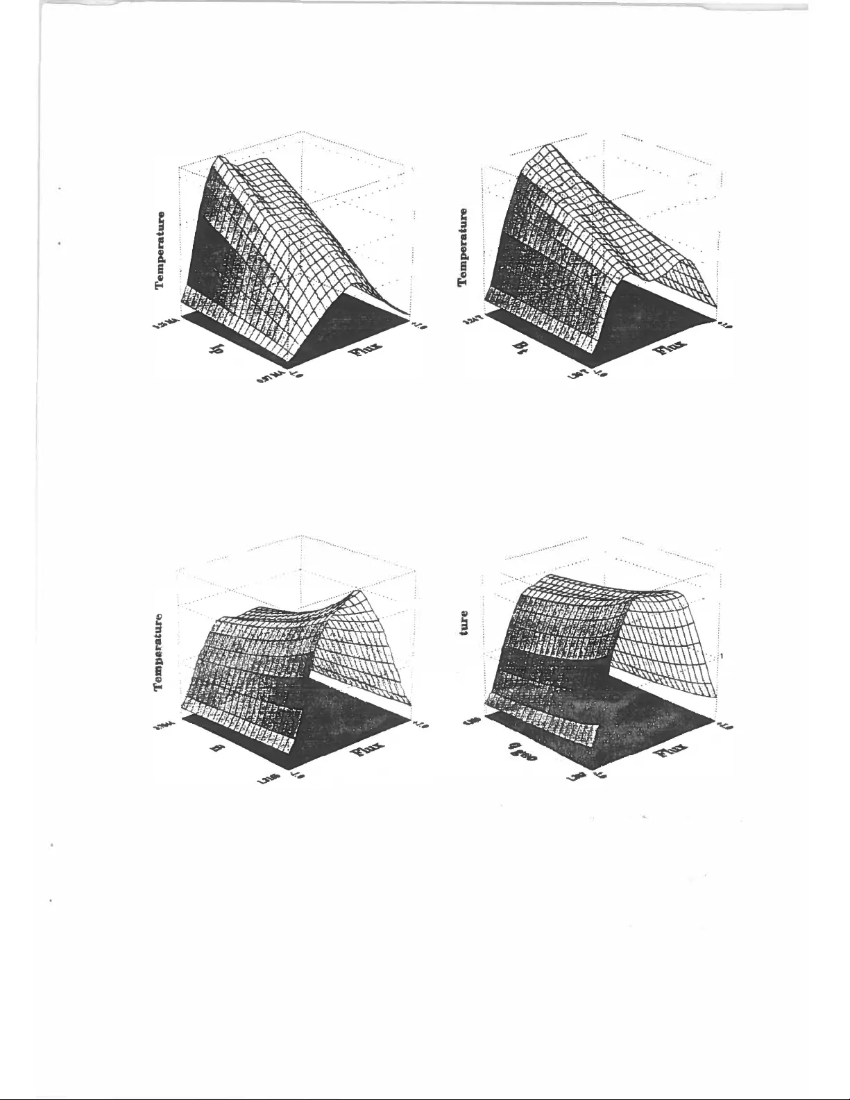
A HIERAR CHY OF EMPIRICAL MODELS OF PLASMA PR OFILES AND TRANSPOR T Ka y a Imre and Kurt S. Riedel New Y ork Universit y , 251 Mercer St., New Y ork NY 10012-1185 Beatrix Sc h unk e JET Join t Undertaking, Abingdon, Oxon, O X14 3EA, UK Abstract Tw o families of statistical models of increasing statistical c omplexity are presen ted whic h generalize global confinemen t expressions to plasma profiles and lo cal trans- p ort co efficients. The temp erature or diffusivity is parameterized as a function of the normalized flux radius, ¯ ψ , and the engineering v ariables, u = ( I p , B t , ¯ n, q 95 ) † . The log-additiv e temperature mo del assumes that ln[ T ( ¯ ψ , u )] = f 0 ( ¯ ψ ) + f I ( ¯ ψ ) ln[ I p ] + f B ( ¯ ψ ) ln[ B t ] + f n ( ¯ ψ ) ln[ ¯ n ]+ f q ln[ q 95 ]. The unkno wn f i ( ¯ ψ ) are estimated using smo oth- ing splines. The Rice selection criterion is used to determine whic h terms in the log-linear mo del to include. A 43 profile Ohmic data set from the Join t European T orus [P . H. Rebut, et al., Nuclear F usion 25 1011, (1985)] is analyzed and its shap e dep endencies are describ ed. The b est fit has an av erage error of 152 eV whic h is 10.5 % p ercent of the t ypical line a v erage temp erature. The a verage error is less than the estimated measurement error bars. The second class of mo dels is log-additive dif- fusivit y mo dels where ln[ χ ( ¯ ψ , u )] = g 0 ( ¯ ψ ) + g I ( ¯ ψ ) ln[ I p ] + g B ( ¯ ψ ) ln[ B t ] + g n ( ¯ ψ ) ln[ ¯ n ]. These log-additive diffusivit y mo dels are useful when the diffusivit y is v aried smoothly with the plasma parameters. A p enalized nonlinear regression tec hnique is recom- mended to estimate the g i ( ¯ ψ ). The physics implications of the tw o classes of mo dels, additiv e log-temp erature mo dels and additiv e log-diffusivity mo dels, are differen t. The additive log-diffusivity mo dels adjust the temp erature profile shap e as the radial distribution of sinks and sources. In con trast, the additive log-temp erature mo del predicts that the temp erature profile dep ends only on the global parameters and not on the radial heat dep osition. P ACS NUMBERS: 02, 52.55F a, 52.55Pi, 52.65+z I. INTR ODUCTION Global confinement expressions hav e prov en useful in understanding and predict- ing plasma p erformance 1 − 7 . These confinement expressions are straightforw ard to analyze statistically , but do not address the radial v ariation of the plasma profiles 1 and plasma transp ort co efficien ts. In this article, w e describ e t w o families of empiri- cal mo dels which generalize global scaling expressions to profiles and diffusivities. W e define the m vector, u , to b e a vector of global engineering v ariables. Typically , the comp onen ts of u are the logarithms of the edge safety factor, q 95 , the plasma curren t, I p (in MA), the toroidal magnetic field, B t (in T esla), the line a v erage densit y , ¯ n e (in 10 19 /m 3 ), the absorb ed p o wer, P (in MW), the effective ion c harge, Z ef f , the isotop e mixture, M , the plasma elongation, κ , and the ma jor and minor radii. Other engineering v ariables can include the div ertor configuration, the wall t yp e, and the type of heating. In practice, we usually w ork with the logarithms of the engineering v ariables, and normalize the v ariables ab out their mean v alues in the data set. In this notation, the standard p ow er law for the energy confinement time, τ E , is τ E = c 0 I β 1 p B β 2 t n β 3 . . . , where β ` are the scaling exp onents. The p ow er law can b e rewritten as a log-linear expression ln τ = β 0 + β I ln[ I p ] + β n ln[ n ] + . . . . (1) In this form, the resulting scaling expression can b e analyzed using linear regression. Ordinary least squares analysis mak es a n um b er of implicit assumptions whic h are describ ed in Refs. 1 and 3. W e consider the plasma temp erature as a function of the normalized radial flux v ariable, ¯ ψ , and the plasma control v ariables, u . A conv enient flux v ariable normal- ization is that the toroidal flux through a giv en radius, ¯ ψ , is equal to ¯ ψ 2 times the total flux. In this section, we neglect the random errors asso ciated with the data and concen trate on the empirical mo del. By writing T ( ¯ ψ , u ), we are implying that the temp erature is an unkno wn function of m + 1 v ariables. Attempting to estimate an arbitrary m + 1 dimensional function from the measured tok amak data is a v ery ill-conditioned problem. Therefore, we r estrict the class of mo dels which we examine to a mor e limite d class. Exp erimen talists hav e often observ ed that the Ohmic temp erature profile shap e v aries very little as the plasma con trol v ariables v ary . This “profile resilience” moti- v ates us to define “profile resilien t” mo dels: ln[ T ( ¯ ψ , u )] = f 0 ( ¯ ψ ) + H ( u ) . (2) H ( u ) is indep endent of ¯ ψ and c hanges the magnitude but not the shap e of the tem- p erature profile. In the log-linear case, H ( u ) = c I ln[ I p ] + c B ln[ B t ] + c n ln[ n ] + . . . . W e determine f 0 ( ¯ ψ ) and H ( u ) b y fitting f 0 ( ¯ ψ ) with smo othing splines and using linear regression. 2 A more general mo del is to let the shap e dep end on q 95 : ln[ T ( ¯ ψ , u )] = f 0 ( ¯ ψ ) + f q ( ¯ ψ ) q 95 + H ( u ) , (3) where b oth unknown radial functions, f 0 ( ¯ ψ ) an d f q ( ¯ ψ ), are fit with smo othing splines. T ang’s well-kno wn transp ort mo del 8 , 9 , based on profile consistency , is a sp ecial case of mo del of Eq. (3). T ang’s mo del requires the log-temp erature profile shap e to b e b e quadratic: ( f 0 ( ¯ ψ ) ≡ c 0 ¯ ψ 2 and f q ( ¯ ψ ) ≡ c q ¯ ψ 2 ), and derives H ( u ) from theoretical consideration. More generally , we hav e the additive spline mo del of Refs. 10 − 12: ln[ T ( ¯ ψ , u )] = f 0 ( ¯ ψ ) + H ( u ) + L X ` =1 f ` ( ¯ ψ ) h ` ( u ) . (4) In Eq. (4), w e ha v e separated f 0 ( ¯ ψ ) and H ( u ) from the other terms to stress that these terms are the “profile consisten t” terms. If desired, additional cross-terms ma y b e added to Eq. (4). In Section I I, we describ e our fitting procedure for estimating the free parameters in the log-additive mo del of Eq. (4). In Section I I I, w e apply our metho d to the Ohmic data from the Joint Europ ean T orus 13 (JET) with h ( u ) = (ln[ I p ] , ln[ B t ] , ln[ ¯ n ] , ln[ q 95 ]). The resulting mo del can b e rewritten as T ( ¯ ψ ) = µ 0 ( ¯ ψ ) I f 1 ( ¯ ψ ) p B f 2 ( ¯ ψ ) t ¯ n f 3 ( ¯ ψ ) q f 4 ( ¯ ψ ) 95 , (5) with µ 0 ( ¯ ψ ) = exp( f 0 ( ¯ ψ )). In place of q 95 in Eq. (5), w e can use the geometric part of the safet y factor: ˆ q g eo ≡ q 95 I p /B t . W e also find that a simpler mo del with “ f 1 , f 2 , and f 3 = constan t” fits the data to reasonable precision. In Sections IV and V, we introduce a second family of mo dels for the log-diffusivity . W e summarize our results in Sec. VI. The app endix describ es our mo del selection criteria; i.e. how w e use the data to determine which log-linear mo del is most appro- priate. I I. PROFILE ESTIMA TION AND MODEL SELECTION T o estimate the unkno wn functions, f ` ( ¯ ψ ) in the additiv e log-temp erature mo dels, w e expand each of the functions in B-splines: f ` ( ¯ ψ ) = P K k =1 α `k B k ( ¯ ψ ), where the B k ( ¯ ψ ) are the cubic B-spline functions. The α `k are free parameters which need to b e estimated. In Refs. 10-12, w e describ e how estimation of the unkno wn functions in the log-additive temp erature mo del can b e form ulated as a large linear regression 3 problem. In Ref. 12, w e sho w ho w a smo othness p enalty function can b e used to adv an tage in the spline fit to the additive log-temp erature mo del. W e denote the fitted resp onse function by ˆ T ( ¯ ψ , u | f 0 , . . . , f L ). The algorithm of Ref. 12 is simply: Minimize with resp ect to the B-spline co efficients of f 0 ( ¯ ψ ) , . . . , f L ( ¯ ψ ) of Eq. (4), the w eigh ted least squares problem: X i,j       T i ( ¯ ψ i j ) − ˆ T ( ¯ ψ i j , u i | f 0 , . . . , f L ) σ i,j       2 + L X ` =0 λ ` Z 1 0 | f 000 ` ( ¯ ψ ) | 2 d ¯ ψ , (6) where T i ( ¯ ψ i j ) is the j th radial measurement of the i th measured temp erature profile and σ i,j is the asso ciated error. The second term is the smo othness penalty which damps artificial oscillations in the estimated f ` ( ¯ ψ ). The smo othing parameter, λ ` , con trols the smo othness of the estimate of f ` ( ¯ ψ ). The app endix describ es how we determine λ ` empirically . There are tw o types of systematic error: mo del error (since the additiv e mo del is only an appro ximation), and smo othing error from the smo othness p enalty function. Simplifying the physical mo del causes bias error, but can often reduce the v ariance of the fitted mo del. This v ariance reduction o ccurs b ecause the simplified mo del usually has few er free parameters than a more complete mo del do es. W e wish to choose the additive mo del whic h minimizes the error in predicting the temp erature of a new profile. Unfortunately , the prediction error dep ends on the unkno wn “true” temp erature function. T o select the b est mo del and smo othing parameters, the exp ected av erage square error (EASE) is estimated empirically 14 , 15 . W e use a generalization of the estimate of the EASE given by the Rice criterion. (See the app endix.) This EASE estimate includes the bias error asso ciated with the in- complete mo del, i.e. we admit that our additive mo del is systematically wrong, and w e estimate the size of this error. F rom this estimate of the EASE, w e then select the additiv e mo del whic h min- imizes the Rice criterion. Similarly , w e choose the smo othing parameters, λ ` , to minimize this empirical estimate of the exp ected error. The Rice criterion estimates the fit error for new data while the older “ χ 2 ” statistic considers the fit qualit y for the existing data set. The Rice criterion is more selectiv e than the χ 2 statistic in the sense that it prefers simpler, lo w er order mo dels. I I I. JET OHMIC TEMPERA TURE PROFILE P ARAMETERIZA TION a) Single Pr ofile A nalysis 4 W e consider a 43 profile data set from the Joint Europ ean T orus 13 . The electron temp erature and density profiles are measured b y the JET LIDAR Thomson scatter- ing diagnostic. Eac h profile is measured at appro ximately 50 radial lo cations along the plasma mid-plane. T able 1 summarizes the global parameters of the data. The data con tains disc harges with the edge safety factor, q 95 , as high as 12. The JET discharges w ere pro duced b et w een 1989-90 and 1991-92. During this time, JET op erated with carb on tiles, with carb on tile and b eryllium ev ap oration, and with b eryllium tiles. Most of the discharges in the database ha ve the plasma b oundary formed by the outer wall limiter with b eryllium tiles. The JET LID AR Thomson scattering diagnostic is describ ed in Ref. 16. A n um b er of the profiles hav e an artificial increase in the measured temp erature near the inner w all. This problem o ccurs b ecause the laser ligh t from the LID AR diagnostic is partially reflected near the plasma wall and stimulates radiation emission near the plasma edge. T o prev ent these spurious data from influencing the profile fit, w e delete measuremen ts in the outer ten p ercen t of the plasma whic h ha v e the temp erature increasing near the w all. Near the in b oard wall, there are only rarely usable measurements. T o b e able to estimate the temp erature for ¯ ψ < − 0 . 87, we reflect the temp erature for ¯ ψ > +0 . 87. In our mo del selection criterion, we use the num b er of measured data p oin ts and not the n um b er of augmen ted data. Neither the fitted functions, ˆ f ` ( ¯ ψ ), nor the measured data are symmetric with resp ect to ¯ ψ . The measured profiles are clearly hotter and broader at the in b oard side (negative ¯ ψ ). Since the LIDAR measurements near the inner w all tend to b e less accurate than those on the outb oard side, w e prefer to fit the data with an asymmetric profile. If a symmetric fit is desired, we recommend using our fit restricted to ¯ ψ ≥ 0. It is unclear if this asymmetry is due to a systematic error in the flux map or in the LID AR measuremen ts or has an unknown physical cause. Our fitted profiles allo w asymmetry and repro duce this asymmetry . W e do test eac h f ` separately for symmetry . Making f 1 ( ¯ ψ ) . . . f 4 ( ¯ ψ ) symmetric in ¯ ψ while keeping f 0 ( ¯ ψ ) asymmetric in our b est fit mo del raises the fit error only slightly from 150 to 152 eV. If we force f 0 ( ¯ ψ ) to b e symmetric, the difference in the residual fit error is noticeable. In our spline fits, we use 20 knots. T o reduce the ill-conditioning of the fit near the plasma edge, we decrease the densit y of knots near the edge. Our profile fits dep end only v ery weakly on the knot spacing due to the smo othness p enalty term. In con trast, if no smoothness penalty is used (as in the original algorithm of Refs. 10-11), the fit is strongly influenced b y knot selection. Our data fit give an accurate fit to 5 the data whic h is nearly indep endent of the knot p ositions. The smo othing spline yields accurate representation of the solution with few er artificial oscillations than the metho dology of Ref. 10. Fitting each profile separately gives a ro ot mean square error (RMSE) of .171 on the logarithmic scale, which corresp onds to a relative fit error of 17.1% . On the linear scale the a verage fit error is 152 eV which is 10.5% p ercent of the typical line a v erage temp erature (1.454 KeV). The ro ot mean square error (RMSE) is m uc h larger (187 eV) than the mean absolute error, indicating that a small p ercen tage of the data p oin ts are b eing fit v ery p o orly . F or the individual fits, the Rice criterion selects a relatively small amount of smo othing and the fit tends to follow the small scale oscillations in the data. b) Mo del Sele ction W e b egin b y considering the profile consistency mo del of Eq. (2): ln[ T ] = f 0 ( ¯ ψ ) + c I ln[ I p ] + c B ln[ B t ] + c n ln[ ¯ n ] + c κ ln[ κ ] + c a ln[ a ] . (7) This profile consistency mo del has a Rice criterion v alue of 1.26. This is 42% larger than our final nonparametric fit in Eq. (8). Th us, the spatial dep endencies ln[ I p ], ln[ B t ] and ln[ ¯ n ] are significan t. W e now consider nonparametric models whic h include spatial v ariation in the con trol v ariable dep endencies. T o select our log-linear mo del, we use a selection pro cedure based on the Rice criterion. Our list of candidate v ariables is ln[ I p ], ln[ B t ], ln[ ¯ n ], ln[ q 95 ], ln[ κ ], Z ef f , V loop , a , R , ` i , and time. A t the ` -th stages, we try all p ossible combinations of the b est mo del at the ( ` − 1)-th stage plus one additional v ariable. W e c ho ose the mo del whic h reduces the Rice criterion the most. T able 2 summarizes the reduction in the Rice criterion at each stage. ln[ I p ] is clearly the most imp ortan t con trol v ariable. This result contrasts with earlier profile consistency studies 12 , 17 whic h found that the edge safety factor, q 95 , is the most im- p ortan t v ariable in determining the temp erature profile shap e. This difference o ccurs b ecause we are fitting the unnormalized temp erature and I p is m uch more imp ortant than q 95 in determining the magnitude of the temp erature. A t the second stage of the sequen tial selection pro cedure, the pair (ln[ I p ] , ln[ B t ]) minimizes the Rice criterion. In the second column of T able 2, we compare the tw o con trol v ariable mo del: using f I ( ¯ ψ ) ln[ I p ] + f B ( ¯ ψ ) ln[ B t ] with the tw o con trol v ariable mo del and using f I ( ¯ ψ ) ln[ I p ] + f q ( ¯ ψ ) ln[ q 95 ], and we show that the Rice criterion is lo w er when I p and B t are used. The same result holds when ln[ n ] is added to b oth mo dels. A t the third stage, (ln[ I p ] , ln[ B t ] , ln[ ¯ n ]) has the lo west v alue of the Rice 6 criterion. A t the fourth stage, ln[ q 95 ] had the lo w est v alue of the Rice criterion when paired with the “seed v ariables”, (ln[ I p ] , ln[ B t ] , ln[ ¯ n ]). Initially , we had difficulty accepting this result b ecause the I p and B t dep endencies of q 95 w ere already accounted for in the mo del and the geometric parameters, κ , a and R v ary v ery little. T o test if this result were real, w e explicitly remo ved the I p and B t dep endencies from q 95 b y defining ˆ q g eo ≡ q 95 I p /B t . W e found that adding ln[ ˆ q g eo ] resulted in an ev en smaller v alue of the Rice criterion than adding ln[ q 95 ]. This o ccurs b ecause f ˆ q geo ( ¯ ψ ) v aries less than f q 95 ( ¯ ψ ). As a result, we use fewer effective degrees of freedom to represent f ˆ q geo ( ¯ ψ ). In general, adding a fifth v ariable resulted in little reduction in the Rice criterion, and the new function, f 5 ( ¯ ψ ), would b e nearly constan t with large error bars. As a result, w e stopp ed the log-linear expansion with four con trol v ariables. Our final mo del is ln[ T ] = f 0 ( ¯ ψ ) + f I ( ¯ ψ ) ln[ I p /I 0 ] + f B ( ¯ ψ ) ln[ B t /B o ] + f n ( ¯ ψ ) ln[ ¯ n/n o ] + f q ( ¯ ψ ) ln[ ˆ q g eo / ˆ q ] , (8) where ˆ q g eo ≡ q 95 I p /B t , I o = 2 . 552, B o = 2 . 710, n o = 2 . 171, and ˆ q = 4 . 150. T able 3 ev aluates f 0 ( ¯ ψ ) . . . f 4 ( ¯ ψ ) at equispaced in terv als. A t the cost of increasing the fit error by 6 % (from 150 to 159 eV), we can replace the mo del of Eq. (8) with the simpler mo del ln[ T ] = f 0 ( ¯ ψ ) + f q ( ¯ ψ ) ln[ q 95 / 4 . 537] + c I ln[ I p /I 0 ] + c B ln[ B t /B o ] + c n ln[ ¯ n/n o ] , (9) where c I , c B and c n are independent of ¯ ψ . The best fit v alues are c I = 0 . 69, c B = 0 . 49, c n = − . 37 and f q ( ¯ ψ ) ≈ − 0 . 2 for | ¯ ψ | < 0 . 66 and decreasing to − . 37 at the edge. This simpler mo del may b e more robust than the b est fit mo del of (8). The fit functions for b oth Eq. (8) and Eq. (9) are a v ailable from the authors. c) Fit R esults Figure 1 plots exp( f 0 ( ¯ ψ )) and the f ` ( ¯ ψ ). exp( f 0 ( ¯ ψ )) is the predicted temp erature at I p = I 0 , B T = B 0 etc. f I ( ¯ ψ ) shows that the temp er atur e br o adens and b e c omes somewhat hol low with incr e asing curr ent while f B ( ¯ ψ ) sho ws the same effect with decreasing toroidal magnetic fields. If f B ( ¯ ψ ) = c − f I ( ¯ ψ ), then the shap e of the profile would dep end only on the ratio, B t /I p . Thus the shap e dep ends primarily but not exclusively on B t /I p . f B ( ¯ ψ ) is more p eak ed than f I ( ¯ ψ ) is hollo w, whic h shows that a relativ e change in B t c hanges the shape more than the corresponding change in I p . The sequen tial selection pro cedure selected I p o v er B t in the first step b ecause I p v aried more than B t . Thus using I p reduced the fit error more. f ˆ q geo ( ¯ ψ ) is less p eak ed 7 than either f B ( ¯ ψ ) or f I ( ¯ ψ ), and therefore c hanging q 95 b y c hanging the geometry ( a , R and κ ) only weakly changes the profile shap e. f n ( ¯ ψ ) and f ˆ q geo ( ¯ ψ ) are roughly constan t, whic h means that n and ˆ q g eo ha v e little effect on the shap e of the temp erature profile. When f n ( ¯ ψ ) and f ˆ q geo ( ¯ ψ ) are replaced b y constants, the mean absolute residual fit error increases from 150 eV to 156 eV. These constants are also plotted in Figure 1. Figure 2a plots the fitted temp erature v ersus ¯ ψ and I p at fixed v alues of the other parameters. Figure 2b sho ws ho w the fitted temp erature v aries with B t . Our results differ from earlier “profile consistency” results b ecause w e fit b oth the temp erature shap e and magnitude simultaneously; i.e. w e do not normalize the data. The sequential selection pro cedure shows that the total plasma curren t is more imp ortan t than the edge safety factor in determining the JET Ohmic temp erature profile. F rom the shap e of the f ` ( ¯ ψ ), we see that the p olynomial mo dels of the radial dep endence p o orly appro ximate the actual shap e. Figure 3 plots t wo of the fitted profiles to illustrate the go o dness of fit. Our fitted curv e is generally inside the exp erimen tal error bars. The com bined fit to Eq. (8) giv es a mean absolute error of 152 eV. Since the mean line a v eraged temp erature is 1.454 KeV, this is a 10.5 % typical error. On the logarithmic scale, the RMSE is .171, whic h corresp onds to a relativ e fit error of 17.1 %. The mean square error is relev an t when the errors ha v e a Gaussian distribution. In our fit, a small p ercen tage of the data has muc h larger residual errors than is t ypical. Av eraging the square error instead of a v eraging the absolute error inflates the influence of the p o orly fitting p oints. W e b eliev e that the mean absolute residual is a more relev an t description of the qualit y of fit. The Rice criterion v alue of 0.88 usually means that the exp ected square error in predicting new data is 0.88 times larger than the experimental v ariance. F or indep en- den t errors, the Rice v alue should b e greater than one. Due to the o versampling of the LID AR diagnostic, the measuremen t errors are auto correlated, and w e are able to fit the data with smaller residual fit error. In the app endix, we deriv e a correction for the auto correlation. Nevertheless, w e ascrib e the smallness of our Rice v alue to the spatial auto correlation and p ossibly to uncertain ties in the exp erimen tal error bars. The Rice v alue of 0.88 is surprisingly small, given the simplicit y of our mo del and the div erse set of plasma conditions in the database. Thus, w e consider this small enhancemen t to b e a ma jor success. A surprising result of our analysis is that ` i is not p articularly useful in estimating the temp er atur e . ` i is the measured v alue of the second momen t of the p oloidal magnetic field. If we assume that the curren t distribution is given by Spitzer resistivit y 8 (with a constan t, spatially uniform Z ef f profile) then ` i can b e related to a spatially w eigh ted moment of the temperature distribution. Th us, we w ould exp ect that larger v alues of ` i , corresp onding to p eak ed current profiles, would correlate with p eaked temp erature profiles. Our empirical observ ation of only a weak dep endence of the temp erature shap e on ` i sho ws that the curren t and temp erature profile shap es are partially decoupled. This could b e due to v ariation in Z ef f or due to the empirical resistivit y differing from the Spitzer v alue. A t the fifth stage, “time”, as measured from the b eginning of the discharge, is the next most imp ortan t v ariable. W e would lik e to restrict our analysis to time p oin ts in the flat-top. How ever, there are time p oin ts in the early phase of the curren t ramp down. Adding a time v ariable to our regression analysis corresponds to the ln[ T ]( ¯ ψ , t ) ∼ f 0 ( ¯ ψ ) + f t ( ¯ ψ )( t − ¯ t ). Our estimate of f t ( ¯ ψ ) sho ws that earlier times tend to b e more p eak ed and later times are flatter. More sp ecifically , f time ( ¯ ψ ) strongly resem bles f I ( ¯ ψ ), whic h indicates that the profile shap e is influenced b y the time history of the plasma current. Although our log-additive mo del is designed for the steady state part of the discharge, most of these disc harges ha v e a similar time history . This explains why a nonph ysical v ariable like “time” could reduce the fit error. One of the principal disadv antages of our log-linear temp erature models is that the profile shap e do es not adjust in a physical manner when different time ev olution scenarios are used. Th us, f t ( ¯ ψ ) is an artifact of the standard time history scenario in JET, and w e reject using time as a con trol v ariable. The electron temp erature tends to be hotter with carb on tiles than with b eryllium tiles on the limiter. Our empirical fit giv en in Eq. (8) fits b oth classes of discharges, but the fit parameters were basically determined by the 37 b eryllium disc harges. Giv en a larger data set, w e could quan tify the systematic differences b et ween carb on and b eryllium. There are three divertor discharges in our database. The other 40 profiles are limited by the outer wall. Thus the free functions in our empirical fit of Eq. (8) are determined primarily by the limiter disc harges. W e caution that our results are based on a limited database of 43 JET profiles and that other subsets of the JET data could sho w differen t dep endencies. IV. SEMIP ARAMETRIC MODELS OF THE DIFFUSIVITY Muc h effort has b een devoted to determining the anomalous heat diffusivity as a function of the lo cal v ariables. Hundreds of anomalous transp ort mo dels hav e b een prop osed, none of whic h is widely accepted. In contrast, there is a consensus of what the “stereoty pical” heat diffusit y lo oks like: the heat diffusivity is usually flat in the 9 inner half of the plasma radius and then increases parab olically in the outer half of the plasma. F urthermore, the radial v ariation of the heat diffusivit y profile app ears to dep end only weakly on the plasma parameters. There are exceptions to this general assertion, but w e b eliev e that broad c haracterization of the heat diffusivit y profile has b een supp orted by many empirical studies. In constructing empirical mo dels of the anomalous heat diffusivit y , our basic hy- p othesis is that the single most important v ariable for plasma transp ort analysis is the normalized flux radius. In other words, normalized flux radius is a more imp ortant con trol v ariable than more physical v ariables such as the p oloidal gyro-radius. This assertion is difficult to prov e or dispro v e, so w e conten t ourselves with describing a family of mo dels which are based on this hypothesis. W e also wish to parameterize the observed heat diffusivit y as a function of the engineering v ariables in order to influence design studies. Th us, w e prop ose a second class of mo dels whic h is similar to the temp erature mo dels except that we mo del the log-diffusivity . A “diffusivity consisten t” mo del is ln[ χ ( ¯ ψ , u )] = g 0 ( ¯ ψ ) + H ( u ) . (10) Equation (10) implies that as a result the shap e of χ dep ends solely on radius and that the shap e of diffusivit y is indep endent of b oth the lo cal and global plasma pa- rameters including the temp erature gradien t. Thus, the model is Bohm-like for radial v ariation. W e b elieve that mo dels similar to Eq. (10) appro ximate the exp erimen tal data fairly w ell in the sense that the diffusivit y tends to be flat out to ¯ ψ = . 6, and then increases parabolically . We have not yet mo dele d plasma dischar ges by p ar ameterizing the diffusivity, but similar mo dels have b e en use d in plasma mo deling 19 . In general, the radial v ariation of ln[ χ ] can b e represen ted as a slowly v arying function of flux radius and the engineering v ariables. Therefore, w e generalize Eq. (10) to all log-additiv e mo dels of diffusivit y: ln[ χ ( ¯ ψ , u )] = g 0 ( ¯ ψ ) + L X ` =1 g ` ( ¯ ψ ) h ` ( u ) . (11) The in ward density pinch can b e included with a similar linear mo del. As in Eq. (4), w e assume that the h ` ( u ) are known and are typically ln[ I p ] , ln[ n ] and ln[ B t ]. The g ` ( ¯ ψ ) are usually giv en by other smo othing splines or lo w order p olynomials. The physics implications of the tw o classes of mo dels – additive log-temp erature mo dels and additiv e log-diffusivit y mo dels – are differen t. The additiv e log-diffusivit y mo dels adjust the temp erature profile shape as the radial distribution of sinks and sources. In contrast, the additiv e log-diffusivit y mo del predicts that the temp erature 10 profile shap e do es not dep end only on the global parameters and not on the radial distribution of sinks and sources. Profile resilience can b e interpreted as the observ ation that the truth is somewhere b et w een these t w o viewp oints. In other w ords, the temp erature profile shap e adjusts less than one w ould exp ect from a diffusive mo del 18 . In future work, we hop e to com- pare the t wo classes of mo dels to see whether additiv e shap e mo dels b etter describ e the temp erature on the diffusivity . W e can add additional v ariables to the control v ariable vector, u , suc h as the b eam p enetration depth normalized to the minor radius, whic h partially sp ecify the heating profile. In this w a y , we can hav e additiv e log-temp erature mo dels adjust to heating profiles and additiv e log-diffusivit y mo dels b e more profile resilien t. In the next section, we discuss the underlying difficulties in parameterizing the diffusivit y . V. ESTIMA TION OF THE ADDITIVE LOG-DIFFUSIVITY MODEL T o estimate the B–spline coefficients for the additiv e log-diffusivity mo del, we minimize Eq. (5) as well. F or the additiv e log-temperature mo del, the predicted v alues, ˆ T ( ¯ ψ i j , u i | g ` ), are a linear function of the spline co efficients and the resulting functional is quadratic. In con trast, in the additiv e log-diffusivit y mo del, ˆ T ( ¯ ψ , u | g ` ) is a nonlinear function of the unknown spline co efficien t and each ev aluation of ˆ T ( ¯ ψ , u | g ` ) in the minimization of Eq. (6) requires the solution of the transp ort equation using a co de suc h as SNAP 20 . The sinks and sources may b e calculated for each discharge separately prior to b eginning the least squares fit for the additive log-diffusivity mo del. Th us the ev aluation of ˆ T ( ¯ ψ , u | g ` ) requires only the in version of a heat transp ort equation with fixe d sinks and sour c es at each step of the minimization of Eq. (6). W e are unaw are of an y lo cal χ /heat flux regression study that has attempted to use ¯ ψ and the global engineering v ariables with a mo del similar to Eq. (11). Instead, researc hers hav e tried to determine the dep endencies of the diffusivit y on heat flux b y regressing the p oin t estimates of χ or χ ∇ T v ersus lo cal quantities. Previous lo cal χ /heat flux regressions ha v e ignored ¯ ψ and hav e concen trated on local quantities suc h as the p oloidal gyro-radius. This approach has several disadv antages relativ e to the additiv e log-diffusivit y approac h with a global minimization. First, we b eliev e that the most useful v ariable in fitting the diffusivit y shap es is the normalized plasma radius, ¯ ψ . Second, w e b elieve that usually ln[ χ ] has a simple and smo othly v arying radial dep endence. Third, the errors in estimates of the plasma gradien ts are often 11 comparable to the errors in χ and larger than the errors in the heat flux. When the dep enden t v ariables hav e errors, linear regression is an inconsistent estimator of the parameters. Even worse, the errors of the dep enden t and indep endent v ariables are strongly correlated. Our p ersonal exp erience is that when χ is regressed against ∇ T , the most likely result is that χ ∼ I p V loop n ∇ T . This result is strikingly similar to the definition of χ . Note the similarit y of this expression and the Coppi-Grub er- Mazzucato form ula 21 . In the last paragraph, we describ ed the problems in regressing the local heat flux/ χ v ersus the lo cal plasma parameters instead of radius and the global plasma parameters. W e now describ e a second set of disadv an tages whic h p ersist even when the indep enden t v ariables are ¯ ψ and u . First, by fitting with Eq. (10), w e force χ ( ¯ ψ , u ) to b e a smo othly v arying function. If the estimated χ is regressed at eac h radial p oin t separately , ˆ χ will usually hav e spurious spatial oscillations. Another sev ere disadv antage of regressing the lo cal heat flux/ χ directly is that the heat flux is measured and not inferred. Changing ˆ χ ( ¯ ψ , u ) at one spatial lo cation will mo dify the predicted temp erature, ˆ T , at all radial lo cations. Th us to attain a self-consisten t estimation of χ , w e are forced to fit all radial lo cations simultaneously . Finally , estimates of the v ariance of the p oin t estimate of ˆ χ i ( ¯ ψ i j ) are difficult to obtain, and this mak es a p oin t wise w eighted least squares analysis usually infeasible. F or all these reasons, we prefer the global minimization approac h of Eq. (5) with the simple additive mo del of Eq. (11). Nev ertheless, the computational and programming effort to fit the log-additive χ mo del of Eq. (11) is considerable and w e ha v e not yet applied it to JET data. VI. SUMMAR Y Profile resilience and diffusivity profile resilience strongly suggest that the appro- priate empirical models for lo cal profile dependencies are the additiv e log-temp erature mo del and additive log-diffusivit y mo del. W e therefore distinguish four classes of em- pirical transp ort mo dels: 1) Glob al c onfinement mo dels: τ E (engineering v ariables) as typified by Eq. (1); 2) Semip ar ametric pr ofile mo dels: T ( ¯ ψ , engineering v ariables) as typified by Eq. (8); 3) Semip ar ametric diffusivity mo dels: χ ( ¯ ψ , engineering v ariables) as t ypified b y Eq. (11); 4) First principles tr ansp ort mo dels: T (ph ysics v ariables), p ossibly given b y a theo- retical expression. The h uge m ultiplicit y of transp ort theories and the relative lac k of success in ap- plying theory based mo dels motiv ates us to consider the semiparametric mo dels of 12 classes 2 and 3. W e hop e to use these same mo dels to predict the profile p eaked- ness factor for deuterium-tritium (D-T) disc harges in JET and the tok amak fusion test reactor 22 (TFTR) and for extrap olating p erformance to In ternational T ok amak Exp erimen tal Reactor 23 (ITER). W e ha v e accurately parameterized the JET Ohmic temp erature profiles using a log-linear temperature mo del (Class 2). W e hav e not y et fitted log-additiv e diffusivit y mo dels to the JET data (Class 3). In b oth cases, the s moothing spline co efficien ts are b est determined by minimizing the residual fit error ov er all measured profiles sim ultaneously . Our parameterized temperature mo del, Eq. (8), fits our JET data set with a mean absolute error of 47 eV whic h is 3.2 % percent of the t ypical line a verage temp erature. W e recommend using this parameterization for transp ort analyses and most other applications. Is the database big enough to make these conclusions? Some of our conclusions will dep end on the c hoice of data. If the database w ere to contain only disc harges from a sp ecialized scan on one or tw o consecutiv e days, we w ould probably b e able to fit the data b etter, including detailed profile features. Because our database is taken o v er a diverse set of disc harge conditions, we a v erage o ver the small scale features whic h dep end on the particular discharge conditions. As a result, the fit is worse, but the results are more robust b ecause they reflect man y differen t t yp es of disc harges. The Rice criterion measures the exp ected error in predicting new data, normalized to the v ariance of the measurements for indep endent errors. Our Rice v alue of 0.88 means that our predictions are theoretically more accurate than the exp erimental measuremen ts. This small v alue of the Rice criterion is probably due to the spatial auto correlation from ov ersampling and p ossibly to uncertainties in the exp erimen tal error bars. W e consider this small v alue of the predictive error to b e a ma jor success giv en the diverse set of plasma conditions in the database and the simplicit y of our mo del. Our sequential selection pro cedure sho ws that the curren t is the most imp ortant con trol v ariable in determining the temp erature profile. Previous studies, whic h hav e considered the normalized temp erature, hav e found that the edge safety factor is the most imp ortan t control v ariable. Increasing the plasma current results in broader, often hollo w profiles. Fig. 1 shows that the current and the magnetic field mo dify the profile shap e in different wa ys. Th us, the temp erature shap e do es not dep end exclusiv ely on q 95 . The profile parameterization in Eq. (8) is only for time-indep endent profiles. The log-linear diffusivity mo del ma y b e more relev an t to mo deling time ev olution. Since 13 our database consist almost exclusively of limiter discharges, we are unable to deter- mine if the temp erature profile is mo dified when a divertor is used. APPENDIX: RISK ESTIMA TION AND MODEL SELECTION The estimation of risk/exp ected error is critical to our analysis b ecause we use this estimate to select whic h terms to include in our analysis. W e represen t the “true” log- temp erature v alues by the v ector µ and the measured log-temp erature by y ≡ µ +  . W e present the generalized cross-v alidation (GCV) estimate of the exp ected a v erage square error (EASE) as well as the Rice criterion correction. W e consider the linear regression mo del: y = µ +  , µ := X α , ( A 1) where y is the measuremen t v ector, X is the data matrix, α is the parameter vector and  is a vector of random errors with cov ariance matrix Σ . W e define D to b e diagonal matrix which con tains the in ver ses of the v ariances of the measuremen ts: D i,j = Σ − 1 i,i δ i,j . Presently , we do not include the off-diagonal terms in Σ in the minimization, but do comp ensate for this in our mo del selection criterion. By µ := X α , we mean that we mo del µ by X α , but that w e admit that µ = X α is not exact and that this mo del has a systematic error. W e estimate α using the p enalized least squares estimate: ˆ α λ = arg min α n ( y − X α ) † D ( y − X α ) + λ α † S α o , ( A 2) where S is the p enalt y matrix. Equation (A2) is an abstract matrix formulation of Eq. (6). F or brevity , w e denote z † D z by || z || 2 D where z is an arbitrary n -vector. The subscript λ on ˆ α λ denotes the dep endence on the smoothing parameter. Equation (A2) can b e rewritten as ˆ α λ = [ X † D X + λ S ] − 1 X † Dy = G λ X † Dy , ( A 3) where G λ ≡ [ X † D X + λ S ] − 1 . The cov ariance of ˆ α λ is Co v [ ˆ α λ ˆ α † λ ] = G λ K G λ , ( A 4) where K ≡ X † D Σ D X . In addition to the v ariance, Eq. (A3) has a bias/systematic error: E [ µ − X ˆ α λ ]. The dominant source of bias error in our analysis is due to mo del error in the additiv e mo del. The exp ected a v erage square error (EASE) in the fit is E AS E = E [ || µ − X ˆ α λ || 2 D ] = Bias 2 +V ariance = || E [ µ − X ˆ α λ ] | | 2 D +trace[ C G λ K G λ ] , ( A 5) 14 where C ≡ X † D X and trace[ C G λ K G λ ] = trace[ D X Cov [ ˆ α λ ˆ α † λ ] X † ]. W e wish to minimize the EASE. How ever, it is unkno wn and needs to b e estimated. W e denote the av erage square residual of the empirical fit by ˆ σ 2 λ ( λ ) ≡ || y − X ˆ α λ | | 2 / N . The exp ectation of the square residual error is E h || y − X ˆ α λ | | 2 D i = Bias 2 + { trace[ Σ D ] − 2 trace[ K G λ ] + trace[ C G λ K G λ ] } . ( A 6) Note trace[ Σ D ] = N . Equation (A5) computes the error relativ e to the true, unmea- sured v alues while Eq. (A6) uses the measured residuals. As a result, Equation (A5) can be easily estimated from the data b y computing the MSE of the fit using the mea- sured temp erature. In con trast, Eq. (A5) inv olves the unknown, “true” temp erature. The Cra v en-W ahba estimate of the EASE uses Eq. (A6) to estimate Eq. (A5): d E [ || µ − X ˆ α λ || 2 D ] = || y − X ˆ α λ || 2 D − { N − 2 trace[ K G λ ] } . ( A 7) Equation (A7) is particularly v aluable b ecause it includes the systematic error in directions whic h are orthogonal to the column space of X ; i.e. the bias from not including all p ossible terms in the additive mo del. A t λ = 0, trace[ C G λ ] equals the n um b er of fit parameters and decreases monotonically with λ . Using K in place of C comp ensates for the auto correlation of the measuremen ts. The minim um of Eq. (A7) with resp ect to λ satisfies: ∂ λ ˆ σ 2 λ + 2 N ∂ λ trace[ K G λ ] = 0 . ( A 8) Equation (A8) is useful when σ 2 is kno wn. W e now consider the case where the co v ariance of the measuremen ts is kno wn up to an arbitrary constan t: C ov [ y y † ] = σ 2 Σ , where σ 2 is unkno wn and Σ is known. W e con tinue to define D i,j = Σ − 1 i,i δ i,j and k eep the same definitions for G λ , C and K . When σ 2 is unkno wn, w e can estimate it using the Cra v en-W ah ba estimate of σ 2 : d σ 2 C W = || y − X ˆ α λ | | 2 D ( N − trace[ K G λ ]) . ( A 9) In p enalized regression, “ N − trace[ K G λ ]” is referred to as the effectiv e num b er of degrees of freedom. The empirical estimate of Eq. (A8) using the estimate d σ 2 C W is ∂ λ ˆ σ 2 λ + 2 ˆ σ 2 λ N − trace[ K G λ ] ∂ λ trace[ K G λ ] = 0 , ( A 10) whic h implies ∂ λ ( ˆ σ 2 λ (1 − trace[ K G λ ] / N ) 2 ) = 0 . ( A 11) 15 Th us, w e define the generalized cross-v alidation statistic as GC V ≡ N || y − X ˆ α λ || 2 D ( N − trace[ K G λ ]) 2 . ( A 12) Minimizing the GCV criterion of Eq. (A12) sometimes undersmo othes and tends to pic k mo dels with to o man y free parameters 15 . W e refer the reader to Ref. 15 for an empirical comparison of the Rice criterion and the GCV criterion. Therefore, w e replace Eq. (A10) with a mo dified loss estimator based on the Rice criterion: C R ≡ || y − X ˆ α λ || 2 D N − 2trace[ K G λ ] . ( A 13) C R has also b een normalized to the standard error p er data p oint. C R differs from Eq. (A12) by terms of O (trace[ K G λ ] / N ). In our analysis, we minimize Eq. (A13) with resp ect to b oth the choice of control v ariables in the additiv e mo del and the smo othing parameters in a giv en mo del. In Ref. 24, a somewhat different auto corre- lation correction is deriv ed. An older statistic is χ 2 ≡ || y − X ˆ α λ || 2 N − trace[ K G λ ] , whic h corresp onds to the mean square error p er degree of freedom. The χ 2 statistic is useful in optimizing the fit to existing data while the Rice criterion and generalized crossv alidation are useful in minimizing the predictive error for new data. The factor of t wo in the denominator of C R results in smo other mo dels and fewer v ariables in the mo del. A CKNO WLEDGMENTS G. Cordey’s supp ort and encouragemen t are gratefully ac kno wledged. W e thank C. Go wers, P . Nielsen, K. Thomsen, and D. Muir. KI’s work w as supp orted by the U.S. Departmen t of Energy Gran ts No.DE-F G02-92ER54157. KSR’s w ork w as supp orted b y the U.S. Departmen t of Energy Gran ts DE-FG02-86ER-53223 and 91ER54131. 16 REFERENCES 1. K. S. Riedel, S. M. Kay e, Nuclear F usion 30 731 (1990). 2. K. S. Riedel, Nuclear F usion 30 755 (1990). 3. K. S. Riedel, Comments in Plasma Physics and Controlled F usion 12 (1989) 279. 4. P . Y ushmano v, T. T akizuk a, K. S. Riedel, O. J. Kardaun, J. G. Cordey , S. Ka ye and D. P ost, Nuclear F usion 30 (1990) 1999. 5. K. S. Riedel, Nuclear F usion, 31 927 (1991). 6. J. P . Christiansen, J. G. Cordey , O. J. Kardaun, and K. Thomsen, Nuclear F usion, 31 2117 (1991). 7. J. P . Christiansen, J. G. Cordey , K. Thomsen, A. T anga and the JET team, J. C. DeBo o, D. P . Schissel, T. S. T a ylor, and the DI I I-D team, O. J. Kardaun, F. W agner, F. Ryter and the ASDEX team, S.M. Kay e and the PDX and PBX- M teams, Y. Miura and the JFT-2M group Nuclear F usion, 32 (1992) 291. 8. M. H. Redi, W. M. T ang, P . C. Efthimion, D. R. Mikk elsen, G. L. Schmidt, Nuclear F usion 27 2001 (1987). 9. W. M. T ang, Nuclear F usion, 26 1605 (1986). 10. P . J. McCarthy , K. S. Riedel, O. J. Kardaun, H. Murmann, K. Lac kner, Nu- clear F usion 31 (1991) 1595, also Sc alings and Plasma Pr ofile Par ameterisation of ASDEX High Density Ohmic Dischar ges , Max-Planc k-Institut f ¨ ur Plasma- ph ysik Rep ort No. 5/34. 11. O. J. Kardaun, K. S. Riedel, P . J. McCarthy and K. Lackner, Max-Planc k- Institut f ¨ ur Plasma Ph ysik Rep ort No. 5/35, (1990). 12. K. S. Riedel and K. Imre, Comm. in Statistics 22 , 1795 (1993). 13. P . H. Rebut, R. J. Bick erton, B. E. Keen, Nuclear F usion 25 1011, (1985). 14. P . Crav en and G. W ah ba Numer. Math. 31 , (1979) 377. 15. W. Hardle, P . Hall, and S. Marron, J. Amer. Statist. Asso c. 83 (1988) 86. 17 16. H. Salzmann, J. Bundgaard, A. Gadd, C. Go w ers, P . Nielsen, Rev. Sci. Instrum. 59 , (1988) 1451. 17. V. D. Arunsalam, N. L. Bretz, P . C. Efthimion, R. J. Goldston, B. Grek, D. W. Johnson, M. Murak ami, K. M. McGuire, D. A. Rasmussen, F. J. Stauffer and J. B. Wilgen Nuclear F usion 30 (1990) 2111. 18. C. K. Phillips, W. Houlb erg, D. Hwang, S. A ttenberger, J. T olliver, L. Hively , Plasma Ph ys. Con trol. F usion 35 (1993) 301. 19. J. P . Christiansen, J. D. Callen, J. G. Cordey , K. Thomsen, Nuclear F usion 28 (1988) 817. 20. H. H. T o wner, R. J. Goldston, G. W. Hammett, J. A. Murphy , C. K. Phillips, S. D. Scott, M. C. Zarnstorff, D. Smithe, Reviews of Sci. Inst. 63 ,4753-6, (1992). 21. O. Grub er, Nuclear F usion 22 , (1982) 1349. 22. D. J. Gro ve, D. M. Meade, Nuclear F usion 25 1167, (1985). 23. D. P ost et al. I.T.E.R. Physics Basis. I.A.E.A. Publishing, Vienna, (1991). 24. N. S. Altman, J. Amer. Stat. Asso c. vol. 85, (1990) pp. 749. 18 -�-  -- ,.                           4                       f 1          (8).  1          a                                q                        g                              8 19          I     !,                                    I                     7    =  9    g co =                    0   19   g =                                           r.                                     r 20                  49.01 FE                                                 10 21 WIW47W t iiTh..mi t•1 I I 7I. IW2 III 22 t) 23 ii I L LIIL az II = ii I III — J14 CSI ILfl (I — 4’ Iw £11 1? I IgII PII I IItLLSI NLD (I I LII1MI OP 24 XI Nfll21 I I VtI.IIIW I 14 I4I IN.TINI TI4I, ll*JPl ,.JN FE . TWIl •4 IJII II ii7e2J7 I WU II7 I .I I ?l FE .-:: 17III IiI7 •.I3 e 741 I7I2.NI I 77 Il I7t FkNI !\ 24 25 It7lI I IWZIIII 7EI II II .i a I O ? I I ZIL5 I lI4I I fla 1 T11WLISI IJIl I41I Imaraa1I1u .7I II Ii FRI(La 26 26 27 T ABLES V ar mean min max std dev ¯ n 2.29 1.32 3.90 0.75 q 95 5.48 2.88 12.6 2.86 I p 2.80 0.97 5.25 1.13 B t 2.76 1.30 3.22 0.46 κ 1.44 1.30 1.75 0.122 a 1.16 1.05 1.19 0.040 R 2.92 2.83 3.01 0.047 V olt -.35 -1.12 .914 0.66 Z ef f , 1 1.88 1.07 3.10 0.55 Z ef f , 2 2.10 1.20 3.35 0.60 T able 1: Database Summary: Av erage, minimum, maxim um and standard devi- ation of eac h of the engineering v ariables. 28 Se quential Sele ction Using R ic e Criterion V ars in mo del 1 V ar 2 V ar 3 V ar 4 V ar 5 V ar ln[ ¯ n ] 4.64 1.73 1.12 seed seed ln[ q 95 ] 3.04 1.78 1.36 .885 seed ln[ I p ] 1.93 seed seed seed seed V olt 4.63 1.92 1.53 1.10 .861 ln[ B t ] 3.96 1.58 seed seed seed ln[ κ ] 4.30 1.94 1.56 1.10 .875 ` i 4.21 1.63 1.48 1.05 .875 a 4.60 1.91 1.58 1.11 .865 R 4.47 1.88 1.58 1.06 .869 Z ef f , 1 4.01 1.91 1.55 1.06 .872 Z ef f , 2 4.37 1.79 1.57 1.11 .850 Time 4.58 1.87 1.52 .923 .793 T able 2: Rice criterion as a function of the v ariables in the model. “Seed v ariables” are included in each run in that column. W e then add the v ariable that reduces the criterion the most. 29 Fitted F unctions for Eq. (8) ¯ ψ f 0 ( ¯ ψ ) f I ( ¯ ψ ) f B ( ¯ ψ ) f n ( ¯ ψ ) f ˆ q geo ( ¯ ψ ) -1.0 0.2376 0.5057 0.0776 -0.3013 -0.3879 -0.9 0.4267 0.6679 0.0900 -0.2332 -0.3755 -0.8 0.7972 0.7728 0.1320 -0.2710 -0.3370 -0.7 1.1884 0.8231 0.2037 -0.3479 -0.2902 -0.6 1.4813 0.8236 0.3046 -0.3746 -0.2484 -0.5 1.7071 0.7827 0.4317 -0.3449 -0.2161 -0.4 1.8869 0.7131 0.5771 -0.3294 -0.1891 -0.3 1.9517 0.6316 0.7261 -0.3658 -0.1631 -0.2 1.9528 0.5561 0.8577 -0.4384 -0.1397 -0.1 1.9785 0.5029 0.9491 -0.5021 -0.1236 0.0 2.0271 0.4838 0.9820 -0.5261 -0.1179 0.1 2.0257 0.5029 0.9491 -0.5021 -0.1236 0.2 1.9588 0.5561 0.8577 -0.4384 -0.1397 0.3 1.8611 0.6316 0.7261 -0.3658 -0.1631 0.4 1.7285 0.7131 0.5771 -0.3294 -0.1891 0.5 1.5236 0.7827 0.4317 -0.3449 -0.2161 0.6 1.2578 0.8236 0.3046 -0.3746 -0.2484 0.7 0.9711 0.8231 0.2037 -0.3479 -0.2902 0.8 0.6821 0.7728 0.1320 -0.2710 -0.3370 0.9 0.4173 0.6679 0.0900 -0.2332 -0.3755 1.0 0.2243 0.5057 0.0776 -0.3013 -0.3879 T able 3: Ev aluation of the radial spline functions in Eq. (8) for the JET data. 30 Fitted F unctions for Eq. (9) ¯ ψ f 0 ( ¯ ψ ) f q ( ¯ ψ ) f I ( ¯ ψ ) f B ( ¯ ψ ) f n ( ¯ ψ ) -1.0 0.2326 -0.3729 0.6868 0.4900 -0.3652 -0.9 0.4279 -0.3364 0.6868 0.4900 -0.3652 -0.8 0.8015 -0.2822 0.6868 0.4900 -0.3652 -0.7 1.1914 -0.2298 0.6868 0.4900 -0.3652 -0.6 1.4827 -0.1951 0.6868 0.4900 -0.3652 -0.5 1.7092 -0.1836 0.6868 0.4900 -0.3652 -0.4 1.8890 -0.1885 0.6868 0.4900 -0.3652 -0.3 1.9514 -0.1995 0.6868 0.4900 -0.3652 -0.2 1.9505 -0.2105 0.6868 0.4900 -0.3652 -0.1 1.9750 -0.2186 0.6868 0.4900 -0.3652 0.0 2.0194 -0.2215 0.6868 0.4900 -0.3652 0.1 2.0154 -0.2186 0.6868 0.4900 -0.3652 0.2 1.9511 -0.2105 0.6868 0.4900 -0.3652 0.3 1.8579 -0.1995 0.6868 0.4900 -0.3652 0.4 1.7298 -0.1885 0.6868 0.4900 -0.3652 0.5 1.5275 -0.1836 0.6868 0.4900 -0.3652 0.6 1.2613 -0.1951 0.6868 0.4900 -0.3652 0.7 0.9729 -0.2298 0.6868 0.4900 -0.3652 0.8 0.6841 -0.2822 0.6868 0.4900 -0.3652 0.9 0.4194 -0.3364 0.6868 0.4900 -0.3652 1.0 0.2208 -0.3729 0.6868 0.4900 -0.3652 T able 4: Ev aluation of the radial spline functions in Eq. (9) for the JET data. 31