Linear Regression from Strategic Data Sources

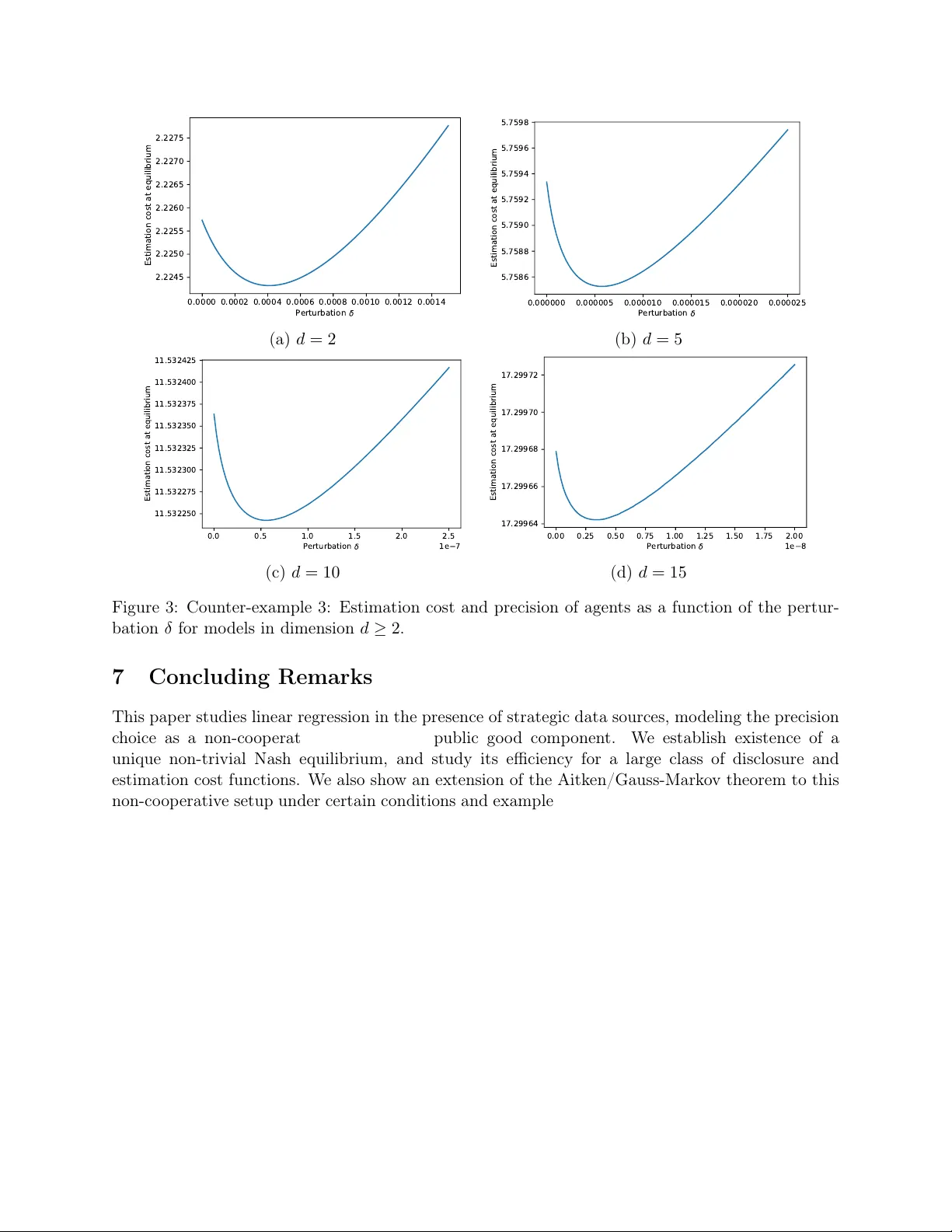
Linear Regression from Strategic Data Sources ∗ † Nicolas Gast 1 , Stratis Ioannidis 2 , P atric k Loiseau 1,3 , and Benjamin Roussillon 1 1 Univ. Grenoble Alpes, Inria, CNRS, Grenoble INP , LIG 2 Northeastern Univ ersit y 3 Max-Planc k Institute for Soft w are Systems (MPI-SWS) Decem b er 16, 2019 Abstract Linear regression is a fundamen tal building blo c k of statistical data analysis. It amoun ts to estimating the parameters of a linear mo del that maps input features to corresponding outputs. In the classical setting where the precision of eac h data p oin t is ﬁxed, the famous Aitk en/Gauss- Mark ov theorem in statistics states that generalized least squares (GLS) is a so-called “Best Lin- ear Un biased Estimator” (BLUE). In modern data science, ho wev er, one often faces str ate gic data sour c es , namely , individuals who incur a cost for providing high-precision data. F or instance, this is the case for p ersonal data, whose revelation may aﬀect an individual’s priv acy—which can b e mo deled as a cost—or in applications such as recommender systems, where pro ducing an accurate estimate entails eﬀort. In this pap er, we study a setting in which features are public but individuals choose the precision of the outputs they reveal to an analyst. W e assume that the analyst p erforms linear regression on this dataset, and individuals b eneﬁt from the outcome of this estimation. W e mo del this scenario as a game where individuals minimize a cost comprising t wo comp onen ts: (a) an (agen t-sp eciﬁc) disclosure cost for pro viding high-precision data; and (b) a (global) estimation cost representing the inaccuracy in the linear mo del estimate. In this game, the linear mo del estimate is a public goo d that b eneﬁts all individuals. W e establish that this game has a unique non-trivial Nash equilibrium. W e study the eﬃciency of this equilibrium and we prov e tight b ounds on the price of stability for a large class of disclosure and estimation costs. Finally , w e study the estimator accuracy achiev ed at equilibrium. W e sho w that, in general, Aitken’s theorem do es not hold under strategic data sources, though it do es hold if individuals ha v e iden tical disclosure costs (up to a multiplicativ e factor). When individuals hav e non-iden tical costs, we derive a b ound on the improv ement of the equilibrium estimation cost that can b e ac hieved by deviating from GLS, under mild assumptions on the disclosure cost functions. Keyw ords: Linear regression, Aitk en theorem, Gauss-Marko v theorem, strategic data sources, p oten tial game, price of stability ∗ This pap er is an extended version of “Linear regression as a non-co op erative game”, b y Ioannidis and Loiseau [29]. † This work w as supp orted by the F renc h National Researc h Agency through the “Inv estissements d’av enir” pro- gram (ANR-15-IDEX-02) and through grant ANR-16-TERC0012; b y the DGA; by the Alexander von Humboldt F oundation; and b y MIAI @ Grenoble-Alp es. Stratis Ioannidis ackno wledges supp ort from NSF grants CCF-1750539 and CNS-1717213. W e thank the editor and the three anon ymous reviewers for their particularly though tful comments and feedback, that signiﬁcantly impro ved the pap er. 1 1 In tro duction The statistical analysis of data is a cornerstone of many scientiﬁc disciplines. The core problem of estimating the parameters of a mo del is classic, and is well understo o d in the standard setting in whic h an y noise or distortions present in the data are exogenous. Naturally , the qualit y of the data, as captured by such noise or distortions, is key to an estimator’s accuracy . In many instances, ho wev er, obtaining high qualit y data ma y b e associated with a cost incurred by the data source. F or example, this is the case when the data is of a p ersonal nature and provided by priv acy-conscious individuals. The quality of the data pro vided in this case can come at a cost of a violation of priv acy [15, 24, 33]. The desire for priv acy incentivizes individuals to obfuscate their priv ate information, or, in the extreme, altogether refrain from any disclosure. An additional setting in which high-quality data may come at a cost is when the data quality dep ends on eﬀort exerted [8, 48], i.e., improv ed quality is the result of increased eﬀort exp ended by the data source. This setting naturally arises in, e.g., op en collab oration pro jects, suc h as wikip edia, but also in online recommender systems, where individuals need to exert eﬀort (complete surveys, click “like” buttons, etc.) to disclose their preferences. Just as in the priv acy case, a data source may choose to not exert the eﬀort required to pro duce high-quality , lo w-noise resp onses or, in the extreme, altogether refrain from reporting anything meaningful. In this setting, where pro viding high-qualit y data comes at a cost, it mak es sense to consider strategic b eha vior among data sources. In particular, one should ask: wh y would strategic data sources pro vide any data at all? The existing literature focuses either on the case where individuals receiv e a monetary compensation to provide data [1, 8, 15, 24, 35, 48], or on the case where individuals care ab out the qualit y of the estimation but only w.r.t. predictions o v er their o wn features [11, 18, 41]. W e consider another p ossibility , namely , that glob al ly suc c essful data analysis may also pr ovide a utility to the individuals fr om which the data is c ol le cte d . This is eviden t in medical studies: an exp erimen t ma y lead to the disco very of a treatment for a disease, from whic h an experiment sub ject may beneﬁt. In the case of recommender systems, users ma y indirectly b eneﬁt from ov erall service impro vemen ts, as data disclosed ma y lead to, e.g., improv ed pro duct recommendations or b etter-targeted advertising. Similarly , op en collab oration pro jects, by their nature, implicitly assume a common underlying utilit y , linked to the success of the collab oration. If such beneﬁts out w eigh asso ciated priv acy or eﬀort costs, individuals may consen t to the collection and analysis of high-qualit y data, e.g., by participating in a clinical trial, completing a survey , or disclosing their preferences in a recommender service. In this pap er, we approach the ab o v e issues through a non-co op erativ e game, fo cusing on the basic statistical analysis task of line ar r e gr ession . W e consider the follo wing formal setting. A set of individuals i ∈ { 1 , . . . , n } participate in an experiment in which they are asked to provide data to an analyst. Each individual i is asso ciated with a feature v ector x i ∈ R d , capturing public information suc h as age, gender, etc., and p ossesses a priv ate v ariable y i ∈ R —e.g., the true answer to a survey , the outcome of a medical test, or how m uc h they lik e a pro duct. The analyst wishes to p erform linear regression o ver the data, i.e., compute a vector β ∈ R d suc h that: y i ≈ β T x i , for all i ∈ { 1 , . . . , n } . W e assume that individuals b eneﬁt from the correct estimation of β : for example, if the analyst learns β , an individual may beneﬁt due to, e.g., b etter medical treatment, impro ved recommenda- tions, etc. Ho w ev er, individuals do not disclose their true priv ate v ariables to the analyst. Instead, they provide a p erturbed version ˜ y i , constructed by adding noise to the priv ate v ariable y i . This is b ecause there is a cost asso ciated with the disclosure of the priv ate v ariable: the higher the v ariance of the noise an individual adds, the low er the cost (e.g., due to priv acy violation or eﬀort exerted) 2 she incurs. On the other hand, high noise v ariance low ers the accuracy of the analyst’s estimate of β , the linear mo del computed in aggregate across multiple individuals. As suc h, the individuals need to strike a balance b et w een the cost they incur through disclosure and the utility they accrue from accurate mo del prediction. W e mak e the following contributions: ( i ) W e mo del interactions b et w een data sources as a non-co op erativ e game, in which each data source selects the precision (i.e., the inv erse of the noise v ariance) of the priv ate v ariable she strategically discloses. A data source’s decision minimizes a cost function comprising t w o comp onen ts: (a) a disclosur e c ost , that is an increasing function of the chosen precision, and (b) an estimation c ost , that decreases as the accuracy of the analyst’s estimation of β increases. F ormally , the estimation cost is a function of the cov ariance matrix of the estimate of β . ( ii ) W e characterize the Nash equilibria of the ab ov e game. In particular, we sho w that it is a p oten tial game and that, under appropriate assumptions on the disclosure and estimation costs, there exists a unique pure Nash equilibrium at which individual costs are ﬁnite. ( iii ) Armed with this result, we determine the game’s eﬃciency , pro viding b ounds for the price of stabilit y for sev eral cases of disclosure and estimation costs. ( iv ) Finally , w e turn our atten tion to the analyst’s estimation algorithm. In the presence of non- strategic data sources, the Aitken theorem 1 states that generalized least squares estimation yields minimal co v ariance among linear un biased estimators. W e c hallenge this theorem in the con text of strategic data sources and obtain b oth p ositive and negative results: a. W e show that, in general, an equiv alent of Aitken theorem no longer holds under strategic data sources. W e exhibit a series of counter-examples that sho w that, when data sources ha v e non-identical disclosure cost functions, there exist linear estimators that lead to more eﬃcien t equilibria (i.e., that attain more accurate estimates at equilibrium) than generalized least squares. b. W e show that, when agents hav e monomial cost functions with identical exp onents (but with p ossibly non-iden tical multiplicativ e factors), then generalized least squares is opti- mal among the class of unbiased linear estimators ev en in the strategic setting: it indeed yields the most accurate estimate at equilibrium. c. Finally , even when generalized least squares is sub optimal, under mild assumptions on the disclosure cost functions, we sho w that the improv ement of the equilibrium estimation cost that can b e achiev ed by deviating from generalized least squares is b ounded b y a factor that dep ends on the heterogeneity of data source disclosure costs. Our results imply that the optimalit y of the generalized least squares estimator does not p ersist if data sources strategically choose the v ariance of their data. More broadly , we model the outcome of a statistical data analysis—the estimator’s accuracy— as a public go o d : data sources con tribute to the public goo d by providing high-precision data at a disclosure cost and b eneﬁt in return from the global estimator’s accuracy . As is natural in suc h public go o d games, we ﬁnd that data sources typically con tribute a level of data precision at equilibrium that is sub optimal from the so cial w elfare p ersp ective (i.e., there is partial free-riding). More surprisingly though, w e also ﬁnd that under such strategic data sources, standard statistics 1 Also known as the Gauss-Marko v theorem in the sp ecial case of ordinary least squares. 3 results are challenged: it is sometimes p ossible to deviate from the standard estimator to increase the public go od provision at equilibrium, without inv olving any monetary comp ensation. The remainder of this pap er is organized as follows. W e present related w ork in Section 2. Section 3 contains a review of linear regression and the deﬁnition of our non-co op erativ e game. W e c haracterize Nash equilibria in Section 4 and discuss their eﬃciency in Section 5. Our results on the optimalit y (or non-optimalit y) of generalized least squares are in Section 6, and our conclusions in Section 7. All pro ofs are relegated to appendices. 2 Related W ork Data P erturbation for Priv acy . P erturbing a dataset b efore submitting it as input to a data mining algorithm has a long history in priv acy-preserving data-mining (see, e.g., [19, 47]). Inde- p enden t of an algorithm, early researc h focused on p erturbing a dataset prior to its public re- lease [21, 46]. P erturbations tailored to sp eciﬁc data mining tasks hav e also b een studied in the con text of, e.g., reconstructing the original distribution of the underlying data [2], building decision trees [2], clustering [40], and asso ciation rule mining [4]. W e approach such p erturbation techniques via a non-coop erative setting, where individuals strategically choose the p erturbation to their data. The ab o ve setting diﬀers from the framework of  -diﬀerential priv acy [22, 32], which has also b een studied from the p ersp ective of mechanism design [39]. In diﬀerential priv acy , noise is added to the output of a computation, which is subsequently publicly released. The analyst p erforming the computation is a priori trusted; as such, individuals submit unadulterated inputs. Sev eral works study mechanisms incen tivizing data disclosure under costs quantiﬁed b y diﬀerential priv acy [15, 16, 24, 33], whereby individuals are comp ensated for the priv acy cost they incur. In con trast, we do not assume that the analyst is trusted, which motiv ates input p erturbation. Such input p erturbations also corresp ond to the more recently studied notion of lo cal diﬀeren tial priv acy [20, 31], though such studies fo cus on the priv acy/utility tradeoﬀ, ignoring the strategic asp ect of the input perturbation. Strategic Data Sources and Data Elicitation. A few recen t works consider settings where sources may c ho ose their eﬀort when generating data [8, 35, 48] or hav e heterogeneous costs due to disclosure [1]. In all these works, data sources are assumed to maximize the paymen t received (min us cost of eﬀort). W e note that in Cai et al. [8] and W estenbroek et al. [48], which are the closest to our work, the disclosure costs of data sources are linear in the exerted eﬀort, whereas w e use more general con vex costs. The data elicitation literature also includes related problems, in whic h one tries to incentivize an exp ert to truthfully rev eal her prediction of an even t, typically using scoring rules [23] (see also the literature on incentiv es in crowdsourcing [17]). A num b er of pap ers also consider data acquisition in sequen tial settings [1, 10, 34]. All this literature, ho w ev er, considers agen ts that aim to maximize the paymen t receiv ed but are insensitive to the quality of the learning result. Moreov er, agents aim to optimize paymen ts while the learning algorithm is ﬁxed; the only exceptions to the latter are [9, 14], which are restricted to the case of a v eraging and do not consider learning tasks such as regression. In contrast, in this work, we do not in v olv e pa yments but assume that data sources b eneﬁt from the result of the learning algorithm. Strategy-Pro of Statistical Inference. Several pap ers study regression from the p ersp ectiv e of mec hanism design, whereb y priv ate v ariables are directly rep orted by strategic agen ts. In particular, Dek el et al. [18] consider a broad class of regression problems in whic h data sources ma y misrep ort their priv ate v alues, and determine loss functions under which empirical risk minimization is group strategypro of. The special case of linear regression is also treated, alb eit in a more restricted 4 setting, by P erote and Perote-P eña [41], who iden tify more general strategypro of mechanisms for the 2-dimensional case. More recen tly , Chen et al. [11] consider a similar setting and prop ose a family of group strategypro of regression mec hanisms for an y dimension, extending the results of b oth [18] and [41]. As in our pap er, those works assume that the indep endent v ariables (the x i ’s) are public information and mostly lo ok at mechanism design without money . Several pap ers also analyze similar problems in the case of classiﬁcation [25, 36] (see also a recent v ariant in [6]). In contrast to this line of research, our work assumes that the analyst uses a ﬁxed algorithm (GLS or a linear unbiased estimator). W e also assume that individuals choose the precision of the data reported (and not directly the rep orted v alue), and no design is required as the c hosen precision is assumed kno wn. The main diﬀerence, how ever, is conceptual: in [11, 18, 41] agents care ab out the estimation error on their instance only , whereas w e assume that agents b eneﬁt equally from the global downstream eﬀects of an accurate predictor. W e consider noise addition as a non-co op erativ e game, fo cusing on pure Nash equilibrium as a solution concept and studying its eﬃciency . Non-Co op erativ e Regression Games. Closer to our setting, Hossain and Shah [28] also con- sider the pure Nash equilibrium as a solution concept in regression games and inv estigate its eﬃ- ciency , albeit in a mo del closer to [11, 18] than to ours. Interestingly , this work considers the mean squared error, a standard quan tity to measure a mo del’s qualit y in linear regression, instead of our estimation cost based on the co v ariance matrix. Our estimation cost, ho wev er, includes a somewhat broader family of functions satisfying mild assumptions (see Assumptions 2 and 4). Our paper is an extended version of “Linear regression as a non-co op erative game”, by Ioannidis and Loiseau [29]. W e generalize and tighten the price of stabilit y results, and correct Theorem 6 of [29] that stated that GLS is optimal for all cost functions. W e show that this result is not true in general but that (i) it holds when agen ts ha v e identical cost functions (up to a multiplicativ e constan t) and (ii) the sub-optimality of GLS in the case of non-iden tical disclosure cost functions can b e bounded under mild assumptions. Exp erimen tal Design. In classic exp erimen tal design [5, 7, 42], an analyst observes the public features of a set of exp eriments, and determines which exp erimen ts to conduct with the ob jective of learning a linear mo del (from non-strategic sources). The qualit y of an estimated mo del is quantiﬁed through a scalarization of its v ariance [7]. As discussed in Section 3.3, man y suc h scalarizations are used in the literature, including the so-called A-optimality , C-optimalit y , and D-optimality criteria we deﬁne in (4). W e fo cus on non-negativ e scalarizations, to ensure meaningful notions of eﬃciency (as determined b y the price of stabilit y in Section 5). Among these classic scalarizations, A-optimalit y and E-optimalit y satisfy b oth our tec hnical assumptions (Assumptions 2 and 4), while D-optimalit y satisﬁes only our conv exity assumption (Assumption 2). As we note in Section 3.3, con v exit y implies that the information gain (i.e., the cost reduction) due to new exp eriments is a submo dular function. This has implications ab out mechanism design as w ell. F or example, Horel et al. [27] exploit this to pro duce a p olytime mec hanism with approximation guarantees for a v ersion of the exp erimental design problem in whic h sub jects rep ort their priv ate v alues truthfully , but ma y lie ab out the costs they require for their participation. Public Go o d Pro vision Problems. W e ﬁnally note that our mo del has analogies to mo dels used in public go o d pro vision problems (see, e.g., [38] and references therein). Indeed, the estimate v ariance reduction can b e seen as a public go o d in that, when a source con tributes data, all other sources in the game beneﬁt. As is standard in suc h literature, our mo del assumes that the disclosure costs (corresp onding to provision costs in public go od problems) and the estimation cost (mapping 5 to the public go o d b eneﬁt) are fully separable. This analogy is pushed further in [12, 13] where the authors prop ose a simple mec hanism to increase the provision of the public go o d at equilibrium in the simple case of a veraging (corresp onding to the standard public go o d framew ork). 3 Mo del Description In this section, w e giv e a detailed description of our linear regression game and the agen ts inv olved. Before discussing strategic considerations, we giv e a brief technical review of linear mo dels, as w ell as key prop erties of least squares estimators; all related results presen ted here are classic (see, e.g., [26]). Notational conv en tions. W e use b oldface t yp e (e.g., x , y , β ) to denote vectors (all vectors are column v ectors), and capital letters (e.g., A , B , V ) to denote matrices. As usual, we denote by S d + , S d ++ ⊂ R d × d the sets of (symmetric) p ositiv e semideﬁnite (PSD) and p ositive deﬁnite matrices of size d × d , resp ectively . F or tw o p ositiv e semideﬁnite matrices A, B ∈ S d + , we write that A  B if A − B ∈ S d + ; recall that  deﬁnes a partial order ov er S d + . W e sa y that F : S d + → R is non-decreasing in the p ositive semideﬁnite order if F ( A ) ≥ F ( A 0 ) for any tw o A, A 0 ∈ S d + suc h that A  A 0 . Moreo ver, we say that a matrix-v alued function F : R n → S d + is matrix c onvex if αF ( λ ) + (1 − α ) F ( λ 0 )  F ( α λ + (1 − α ) λ 0 ) for all α ∈ [0 , 1] and λ , λ 0 ∈ R n . 3.1 Linear Mo dels Consider a set of n data sources, henceforth referred to as agents , denoted by N ≡ { 1 , · · · , n } . Each agen t i ∈ N is asso ciated with a vector x i ∈ R d , the fe atur e ve ctor , whic h is public; for example, this vector ma y corresp ond to publicly av ailable demographic information ab out the agent, suc h as age, gender, etc. Each i ∈ N is also asso ciated with a priv ate v ariable y i ∈ R ; for example, this ma y express the likelihoo d that this agent con tracts a disease, the concen tration of a substance in her blo o d, or a true answer to a survey by that agent. W e assume that the agent’s priv ate v ariable y i is a linear function of her public features x i . In particular, there exists a v ector β ∈ R d , the mo del , suc h that the priv ate v ariables are given by y i = β T x i +  i , for all i ∈ N , (1) where the “inherent noise” v ariables {  i } i ∈ N are i.i.d. 2 zero-mean random v ariables in R with ﬁnite v ariance σ 2 . W e make no further assumptions on the noise; in particular, we do not assume it is Gaussian. An analyst wishes to observ e the y i ’s and infer the mo del β ∈ R d . This type of inference is ubiquitous in experimental sciences, and has a v ariety of applications. F or example, the magnitude of β ’s co ordinates captures the eﬀect that features (e.g., age or weigh t) hav e on y i (e.g., the propensity to get a disease), while the sign of a co ordinate captures p ositive or negative correlation. Knowing β can also aid in prediction: an estimate of priv ate v ariable y ∈ R of a new sample with features x ∈ R d is giv en b y the inner pro duct β T x . W e note that the linear relationship b etw een y i and x i expressed in (1) is in fact quite general. F or example, the case where y i = f ( x ) +  i , where f is a p olynomial function of degree 2, reduces to a linear mo del by considering the transformed feature space whose features comprise the monomials x ik x ik 0 , for 1 ≤ k , k 0 ≤ d . More generally , the same 2 T o ease notation, w e assume that the v ariance of the inheren t noise σ 2 is identical for all agents, but all results of the paper remain v alid if we allow this v ariance (or equiv alently the upp er b ound on the precision 1 /σ 2 , see below) to dep end on the identit y of Agent i . 6 principle can b e applied to reduce to (1) any function class spanned by a ﬁnite set of basis functions o v er R d [26]. 3.2 Generalized Least Squares Estimation W e consider a setup in whic h the agents c ho ose the precision of the data that they provide. That is, they do not directly pro vide y i but rather a p erturb ed v ariable ˜ y i , whic h we assume is an unbiased estimate of y i with v ariance σ 2 i . F or example, in the case of priv acy , agen ts distort their priv ate v ariable b y adding excess noise: each i ∈ N computes ˜ y i = y i + z i where z i is a zero-mean random v ariable with v ariance σ 2 i ; w e assume that { z i } i ∈ N are indep endent, and are also indep enden t of the inheren t noise v ariables {  i } i ∈ N . In the case of eﬀort, the v ariance σ 2 i captures the eﬀort exerted by the agent in generating the lab el ˜ y i . Each agent reveals to the analyst (a) the p erturb ed v ariable ˜ y i and (b) the v ariance σ 2 i . As a result, the aggregate v ariance of the rep orted v alue is σ 2 + σ 2 i and its precision (the in verse of the aggregate v ariance) is λ i ≡ 1 σ 2 + σ 2 i . Note that, as a consequence of the abov e description, our mo del assumes that the analyst can observe the (true) precision of the priv ate data rev ealed by the analyst. This is reasonable in settings where the data is stored in a trusted database and the agen t gran ts access to it under a given precision, and the noise is added by a third party (e.g., the database itself ). In medical researc h for instance, one can imagine that the data is stored in a hospital database; a patien t w ould then grant access to it with a given precision and the analyst would receiv e the p erturb ed data directly from the hospital. In other applications, suc h as surv eys, one can also imagine that, rather than providing a sp eciﬁc v alue, agents would provide an interv al, whose size naturally translates to precision. In turn, ha ving access to the p erturb ed v ariables ˜ y i , i ∈ N , and the corresp onding precisions, the analyst estimates β through gener alize d le ast squar es ( GLS ) estimation. Denote by λ = [ λ i ] i ∈ N the v ector of precisions and by Λ = diag ( λ ) the diagonal matrix whose diagonal is given b y vector λ . Then, the generalized least squares estimator is giv en by: ˆ β GLS = arg min β ∈ R d X i ∈ N λ i ( ˜ y i − β T x i ) 2 ! = ( X T Λ X ) − 1 X T Λ ˜ y , (2) where ˜ y = [ ˜ y i ] i ∈ N is the n -dimensional v ector of p erturb ed v ariables, and X = [ x T i ] i ∈ N ∈ R n × d the n × d matrix whose ro ws comprise the transp osed feature vectors. Throughout our analysis, we assume that n ≥ d and that X has rank d . Note that ˜ y ∈ R n is a random v ariable and as such, by (2), so is ˆ β GLS . It can b e shown that E ( ˆ β GLS ) = β (i.e., ˆ β GLS is un biased), and V ( λ ) ≡ C ov ( ˆ β GLS ) = E h ( ˆ β GLS − β ) T ( ˆ β GLS − β ) i = ( X T Λ X ) − 1 . The co v ariance V captures the uncertain t y of the estimation of β . The matrix A ( λ ) ≡ X T Λ X = P i ∈ N λ i x i x T i is known as the pr e cision matrix. It is p ositiv e semideﬁnite, i.e., A ( λ ) ∈ S d + , but it may not b e in v ertible: this is the case when rank( X T Λ) < d , i.e., the vectors x i , i ∈ N , for whic h λ i > 0 , do not span R d . Put diﬀerently , if the set of agents providing useful information do es not include d linearly indep endent vectors, there exists a direction x ∈ R d that is a “blind sp ot” to the analyst: the analyst has no wa y of predicting the v alue β T x . In this degenerate case the num b er of solutions to the least squares estimation problem (2) is inﬁnite, and the co v ariance is not w ell-deﬁned (it is inﬁnite in all suc h directions x ). Note how ever that, since X has rank d (and hence X T X is in v ertible), the set of λ for which the precision matrix is in vertible is non-empty . In particular, it con tains (0 , 1 /σ 2 ] n since A ( λ ) ∈ S d ++ if λ i > 0 for all i ∈ N . 7 3.3 Non-Co op erativ e Game Mo del of Strategic Data Sources The p erturb ed v ariables ˜ y i are motiv ated by the fact that strategic data sources incur a cost to pro vide high-precision data—for instance, due to priv acy concerns, an agen t may b e reluctant to gran t unfettered access to her priv ate v ariable or release it in the clear. On the other hand, it ma y b e to the agent’s adv antage that the analyst learns the mo del β . In our running medical example, learning that, e.g., a disease is correlated to an agent’s w eight or her c holesterol lev el ma y lead to a cure, whic h in turn may b e b eneﬁcial to the agent. W e model the abov e considerations through cost functions. Recall that the action of eac h agen t i ∈ N amounts to c ho osing the noise level of the p erturbation, captured b y the v ariance σ 2 i ∈ [0 , ∞ ] . F or notational con ve nience, w e use the equiv alent representation λ i = 1 / ( σ 2 + σ 2 i ) ∈ [0 , 1 /σ 2 ] for the action of an agen t. Note that λ i = 0 (or, equiv alently , inﬁnite v ariance σ 2 i ) corresp onds to no participation: in terms of estimation through (2), it is as if this p erturb ed v alue is not rep orted. Eac h agen t i ∈ N chooses her action λ i ∈ [0 , 1 /σ 2 ] to minimize her cost J i ( λ i , λ − i ) = c i ( λ i ) + f ( λ ) , (3) where w e use the standard notation λ − i to denote the collection of actions of all agents but i . The cost function J i : R n + → R + of agent i ∈ N comprises tw o non-negativ e comp onents. W e refer to the ﬁrst comp onen t c i : R + → R + as the disclosur e c ost : it is the cost that the agen t incurs for pro viding the p erturb ed v ariable. The second comp onen t is the estimation c ost , and we assume that it tak es the form f ( λ ) = F ( V ( λ )) , if A ( λ ) ∈ S d ++ , and f ( λ ) = ∞ otherwise. The mapping F : S d ++ → R + is kno wn as a sc alarization [7]. It maps the cov ariance matrix V ( λ ) to a scalar v alue F ( V ( λ )) , and captures how w ell the analyst can estimate the mo del β . The estimation cost f : R n + → ¯ R + = R + ∪ {∞} is the so-called extende d-value extension of F ( V ( λ )) : it equals F ( V ( λ )) in its domain, and + ∞ outside its domain. Main Assumptions. Throughout our analysis, w e mak e the follo wing t w o assumptions: Assumption 1. The disclosur e c osts c i : R + → R + , i ∈ N , ar e non-ne gative, c ontinuous, non- de cr e asing and c onvex. Assumption 2. The sc alarization F : S d ++ → R + is non-ne gative, c ontinuous, incr e asing in the p ositive semideﬁnite or der, and c onvex. The monotonicity assumptions in Assumptions 1 and 2 are standard and natural. Increasing the precision λ i leads to a higher disclosure cost. In contrast, increasing λ i can only decrease the estimation cost: this is because decreasing the v ariance of an agen t’s provided p erturb ed v ariable also decreases the v ariance in the p ositive semideﬁnite sense (as the matrix inv erse is a PSD-decreasing function). The conv exit y assumption in Assumption 2 is also standard and natural. In tuitively , the natu- ralness of Assumption 2 stems from the follo wing observ ation: the con v exity of F implies that the so called information gain , i.e., the relative reduction in F as a new lab el is collected, exhibits a dimin- ishing returns prop erty , as additional lab els aﬀect estimation quality less and less. Scalarizations of p ositive semideﬁnite matrices and, in particular, of the cov ariance matrix V ( λ ) , are abundant in statistical inference literature in the context of exp erimental design [5, 7, 42] (also known as batc h activ e learning). Similar to our setting, in exp erimental design an analyst has access to samples with kno wn feature vectors x i ∈ R d , i ∈ N , and wishes to conduct a limited num b er of k exp erimen ts, where k  N , to collect lab els y i ∈ R for a subset of these samples. Given budget k , the exp eri- men tal design problem amounts to determining which lab els to collect. The standard approach is 8 to accomplish this b y minimizing a scalarization function of the co v ariance of the estimator applied to the labels selected [5, 7, 42]. Three examples of such estimators encountered often in practice are the so-called A-optimalit y , E-optimality , and D-optimality criteria: F 1 ( V ) = trace( V ) , F 2 ( V ) = k V k 2 F , F 3 ( V ) = log det( I + V ) , (4) where k · k F is the F rob enius norm and I is the iden tit y matrix. All three scalarizations satisfy Assumption 2. The con vexit y of these scalarizations implies that, if rep etitions are allow ed (i.e., an exp eriment can b e conducted multiple times), the analyst can determine which fraction of her exp erimen ts should be p erformed on a giv en sample b y solving a conv ex optimization problem (see, e.g., [7]). On the other hand, if rep etitions are not allo w ed, conv exity implies that exp erimental design can b e cast as a submo dular maximization problem sub ject to cardinalit y constraints (see, e.g., [27]), which is NP-hard for the ob jectiv es in (4) but admits a p oly-time approximation. Sub- mo dular maximization arises precisely due to the aforementioned diminishing returns prop erty of the information gain under new lab els; this, in turn, a direct consequence of Assumption 2. Note that, as a further consequence of Assumption 2, the extended-v alue extension f is conv ex (in λ ). The conv exity of F ( V ( · )) follows from the fact that it is the comp osition of the increasing con v ex function F ( · ) with the matrix conv ex function V ( · ) ; the latter is con v ex b ecause the matrix in v erse is matrix con v ex and the precision matrix A ( λ ) is an aﬃne function of λ . A dditional Assumptions. Our result on Nash equilibrium existence and uniqueness (Theorem 1) relies on Assumptions 1 and 2. Our b ounds on the price of stability (Theorem 3) and our Aitk en- t yp e results (Theorem 5) use t w o additional assumptions that further constrain the shap e of the disclosure costs and the scalarization function: Assumption 3. Ther e exist 1 ≤ p min ≤ p max ∈ R + ∪ { + ∞} such that, for al l i ∈ N , the disclosur e c ost c i : R + → R + satisﬁes: a p min c i ( λ ) ≤ c i ( aλ ) ≤ a p max c i ( λ ) , for al l λ ∈ R + and a ≥ 1 . (5) Assumption 4. Ther e exists q ≥ 1 such that the sc alarization F : S d ++ → R + is q -homo gene ous, i.e., it satisﬁes: F ( aM ) = a q F ( M ) , for al l M ∈ S d ++ and a ≥ 1 . (6) In tuitiv ely , Assumption 3 captures “near-homogeneity” of the disclosure cost functions. It is, for example, satisﬁed when all agents hav e monomial disclosure costs c i ( λ ) = r i λ p i , where r i is a constan t, with diﬀerent exp onents p i ∈ [ p min , p max ] . Assumption 4 is also a homogeneity assumption. It holds for a broad class of in teresting scalarizations, suc h as any norm tak en to any p o wer. In particular, it holds for F 1 and F 2 in (4), i.e., the trace and the squared F rob enius norm (with q = 1 and q = 2 resp ectively), whic h are classical scalarizations in the statistical inference literature in the con text of exp erimental design [5, 7, 42]. Note that Assumption 4 also implies that f ( a λ ) = a − q f ( λ ) , for all λ ∈ [0 , 1 /σ 2 ] n and a ≥ 1 . Game notation W e denote by Γ = h N , [0 , 1 /σ 2 ] n , ( J i ) i ∈ N i the game with set of agents N = { 1 , · · · , n } , where eac h each agen t i ∈ N chooses her action λ i in her action set [0 , 1 /σ 2 ] to minimize her cost J i : [0 , 1 /σ 2 ] n → R + , given by (3). W e refer to a λ ∈ [0 , 1 /σ 2 ] n as a str ate gy pr oﬁle of the game Γ . W e analyze the game as a c omplete information game , i.e., w e assume that the set of agen ts, the action sets and utilities are known by all agents. 9 4 Nash Equilibria W e b egin our analysis b y characterizing the Nash equilibria of the game Γ . In the game Γ , eac h agen t c ho oses her con tribution λ i to minimize her cost. A Nash equilibrium (in pure strategy) is a strategy proﬁle λ ∗ satisfying λ ∗ i ∈ arg min λ i J i ( λ i , λ ∗ − i ) , for all i ∈ N . Observ e ﬁrst that Γ is a p oten tial game [37]. Indeed, deﬁne the function Φ : [0 , 1 /σ 2 ] n → ¯ R suc h that Φ( λ ) = f ( λ ) + X i ∈ N c i ( λ i ) , ( λ ∈ [0 , 1 /σ 2 ] n ) . (7) Then for ev ery i ∈ N and for every λ − i ∈ [0 , 1 /σ 2 ] n − 1 , w e ha v e J i ( λ i , λ − i ) − J i ( λ 0 i , λ − i ) = Φ( λ i , λ − i ) − Φ( λ 0 i , λ − i ) , ∀ λ i , λ 0 i ∈ [0 , 1 /σ 2 ] . (8) Therefore, Γ is a p oten tial game with potential function Φ . F rom (8), we see that (as for an y con vex p oten tial game) the set of Nash equilibria coincides with the set of lo cal minima of function Φ . Note that there may exist Nash equilibria λ ∗ for which f ( λ ∗ ) = ∞ . F or instance, if d ≥ 2 , λ ∗ = 0 is a Nash equilibrium. Indeed, in that case, no agen t has an incen tiv e to deviate since a single λ i > 0 still yields a non-inv ertible precision matrix A ( λ ) . In fact, an y proﬁle λ for whic h A ( λ ) is non-inv ertible, and remains so under unilateral deviations, is an equilibrium. W e call such Nash equilibria (at whic h the estimation cost is inﬁnite) trivial . Existence of trivial equilibria can be a v oided using sligh t mo del adjustmen ts: for instance, one can alter the game deﬁnition to disallow inﬁnite v ariances. Alternatively , the existence of d non-strategic agen ts whose feature v ectors span R d is also suﬃcien t to enforce a ﬁnite cov ariance at all λ across strategic agen ts. In the remainder, we fo cus on the more interesting non-trivial equilibria. Using the p otential game structure of Γ , w e derive the following result. Theorem 1. Under Assumptions 1 and 2, ther e exists a unique non-trivial e quilibrium of the game Γ . This result is pro ved in App endix A. The p otential game structure of Γ has another in teresting implication: if agents start from an initial strategy proﬁle λ such that f ( λ ) < ∞ , the so called b est-r esp onse dynamics conv erge tow ards the unique non-trivial equilibrium (see, e.g., [44]). This implies that the non-trivial equilibrium is the only equilibrium reac hed when, e.g., all agents start with non-inﬁnite noise v ariance. 5 Price of Stabilit y Ha ving established the uniqueness of a non-trivial equilibrium in our game, we turn our atten tion to issues of eﬃciency . W e deﬁne the so cial c ost function C : R n → R + as the sum of all agent costs, and sa y that a strategy proﬁle λ opt is so cial ly optimal if it minimizes the so cial cost, i.e., C ( λ ) = X i ∈ N c i ( λ i ) + nf ( λ ) , and λ opt ∈ arg min λ ∈ [0 , 1 /σ 2 ] n C ( λ ) . Let opt = C ( λ opt ) b e the minimal so cial cost. W e deﬁne the pric e of stability ( pric e of anar chy ) as the ratio of the so cial cost of the b est (worst) Nash equilibrium in Γ to opt , i.e., PoS = min λ ∈ NE C ( λ ) opt , and PoA = max λ ∈ NE C ( λ ) opt , 10 where NE ⊆ [0 , 1 /σ 2 ] n is the set of Nash equilibria of Γ . Clearly , in the presence of trivial equilibria, the price of anarc hy is inﬁnity . W e thus turn our attention to determining the price of stabilit y . Note ho w ev er that since the non-trivial equilibrium is unique (Theorem 1), the price of stability and the price of anarch y coincide under the slight mo del adjustments discussed in Section 4 that eliminate trivial equilibria. The fact that our game admits a p oten tial function has the follo wing immediate consequence (see, e.g., [44, 45]): Theorem 2. Under Assumptions 1 and 2, PoS ≤ n . The pro of of Theorem 2 can b e found in App endix B. Impro ved b ounds can b e obtained for sp eciﬁc estimation and disclosure cost functions. The following result provides tighter b ounds when the disclosure costs and the scalarization satisfy Assumptions 3 and 4. Theorem 3. In addition to Assumptions 1 and 2, assume that the disclosur e c ost functions satisfy Assumption 3 with p min ≥ 1 and p max ∈ R ∪ {∞} and that the sc alarization F satisﬁes Assumption 4 for some q ≥ 1 . Then, the pric e of stability satisﬁes PoS ≤ n q p min + q . A dditional ly, for al l p min , q ≥ 1 , and al l ε > 0 , ther e exists a game in which the estimation c ost and the disclosur e c osts satisfy Assumptions 3 and 4, r esp e ctively, such that PoS ≥ n q p min + q (1 − ε ) . The pro of of Theorem 3 can b e found in App endix C. Note that, as the b ound do es not depend on p max , w e can set p max = ∞ in Assumption 3, whic h is equiv alent to replacing this assumption b y a p min c i ( λ ) ≤ c i ( aλ ) , for all λ ∈ R + and a ≥ 1 . The pro of of the upp er b ound relies on deriving a “go o d” solution from the so cial optimum and sho wing that, if the PoS is to o high, this “go o d” solution attains a low er p oten tial than a Nash equilibrium (a con tradiction). The proof of the lo wer b ound in Theorem 3 relies on explicitly c haracterizing the so cially optimal proﬁle in a certain game class, and showing it equals the Nash equilibrium λ ∗ m ultiplied b y a scalar. W e note that the theorem states that, among monomial disclosure costs and for any estimation cost satisfying Assumption 4, the largest PoS is n q 1+ q and is attained for linear disclosure costs. Similarly , among all estimation costs satisfying Assumption 4 and all disclosure costs satisfying the assumptions presented in Theorem 3, the largest PoS is n ; this is approac hed as q tends to inﬁnit y . W e note that a similar worst-case eﬃciency of linear functions among con vex cost families has also b een observed in the context of other games, including routing [43] and resource allo cation games [30]. As such, Theorem 3 indicates that this b eha vior emerges in our linear regression game as w ell but only concerning the disclosure cost: W e observ e a w orst-case eﬃciency of linear functions in this game for the disclosure cost but a worst-case eﬃciency of highly conv ex functions for the estimation cost. 6 An Aitken-T yp e Theorem for Nash Equilibria Un til this p oint, w e ha ve assumed that the analyst uses the generalized least-square estimator (2) to estimate model β . In the non-strategic case, where λ (and, equiv alently , the added noise v ariance) is ﬁxed, the generalized least-square estimator is kno wn to satisfy a strong optimality prop erty: the so- called Aitk en/Gauss-Marko v theorem, which w e brieﬂy review b elow, states that it is a “Best Linear Un biased Estimator”, a prop ert y commonly referred to as BLUE. In this section, w e in vestigate ho w this result extends in the strategic case, i.e., when λ ∗ is not a priori ﬁxed but is the equilibrium reac hed b y agen ts; crucially , the latter dep ends on the estimator used by the analyst. 11 6.1 Linear Un biased Estimators and the Aitk en Theorem A line ar estimator ˆ β L of the mo del β is a linear map of the p erturb ed v ariables ˜ y ; i.e., it is an estimator that can b e written as ˆ β L = L ˜ y for some matrix L ∈ R d × n . A linear estimator is called unbiase d if E [ L ˜ y ] = β (the exp ectation tak en ov er the inheren t and extra noise). Recall by (2) that the generalized least-square estimator ˆ β GLS is an unbiased linear estimator with L = ( X T Λ X ) − 1 X T Λ and cov ariance C ov ( ˆ β GLS ) = ( X T Λ X ) − 1 . Any linear estimator ˆ β L = L ˜ y can b e written without loss of generalit y as L = ( X T Λ X ) − 1 X T Λ + D T , (9) where D = D ( X ) ∈ R d × n , (10) is a matrix that may depend on X but do es not dep end on Λ . It is easy to verify that ˆ β L is un biased if and only if D T X = 0; (11) in turn, using this result, the cov ariance of any linear unbiased estimator can b e shown to b e C ov ( ˆ β L ) = ( X T Λ X ) − 1 + D T Λ − 1 D  C ov ( ˆ β GLS ) . (12) In other w ords, the cov ariance of the generalized least-square estimator is minimal in the p ositiv e- semideﬁnite order among the cov ariances of al l line ar unbiase d estimators . This optimality result is kno wn as the Aitk en theorem [3]. Applied sp eciﬁcally to homoscedastic noise (i.e., when all noise v ariances are identical), it is known as the Gauss-Mark o v theorem [26], which establishes the optimalit y of the ordinary least squares estimator. Both theorems pro vide a strong argumen t in fa v or of using least squares to estimate β , in the presence of ﬁxed noise v ariance (i.e., non-strategic agen ts). 6.2 Extension of the Non-Co op erative Game to Linear Unbiased Estimators Supp ose no w that the data analyst uses a linear un biased estimator ˆ β L with a given matrix L ∈ R n × d whic h may dep end on X . Similarly to the mo del in tro duced in Section 3.3, w e deﬁne a game Γ L in which each agent i chooses her λ i to minimize her cost; this time, how ever, the estimation cost dep ends on the v ariance of ˆ β L . A natural question to ask is the following: it is p ossible that, despite the fact that the analyst uses an estimator that is “inferior” to ˆ β GLS in the BLUE sense, an equilibrium reached under ˆ β L is b etter than the equilibrium reached under ˆ β GLS in terms of equilibrium estimation cost? If so, despite the Aitken theorem, the data analyst would ha ve an incen tiv e to use ˆ β L instead and to inform the agents that she will use ˆ β L and not ˆ β GLS . In this section, w e provide b oth a p ositive and a negative answer to this question, dep end- ing on sp eciﬁc assumptions on the disclosure costs. F ormally , w e consider the game Γ L = h N , [0 , 1 /σ 2 ] n , ( J i ) i ∈ N i deﬁned as in Section 3.3, except that the estimation cost is the extended- v alue extension of F ( V L ( λ )) with V L ( λ ) ≡ ( X T Λ X ) − 1 + D T Λ − 1 D , (Λ = diag λ ) , (13) where D is deﬁned as in (11). Recall that D may dep end on X but do es not dep end on the precision Λ . Then, Γ L is still a p oten tial game with p otential function Φ( λ ) = f L ( λ ) + P i ∈ N c i ( λ i ) where f L ( λ ) = F ( V L ( λ )) . This 12 p oten tial function has the same form as the p otential of the original game, given b y (7). Moreo v er, as the function V L ( · ) giv en by (13) is a matrix con vex function, the extended-v alue extension f L ( · ) is con v ex. This shows that the p otential function is conv ex. Since the pro of of Theorem 1 mostly relies on the con vexit y of the p otential, a straightforw ard adaptation yields the follo wing result. Theorem 4. Under Assumptions 1 and 2, for any line ar estimator L ∈ R n × d , ther e exists a unique non-trivial e quilibrium of the game Γ L . As for the case of GLS , this result follows from the uniqueness of a minimizer of the p otential function attained in the eﬀective domain. In what follo ws, we denote the unique non-trivial equilib- rium of Γ L b y λ ∗ L and w e denote b y λ ∗ GLS the equilibrium of the game Γ with the same parameters except for the estimator. 6.3 Optimalit y of GLS 6.3.1 Theoretical Bound and Optimalit y Condition F or a given linear un biased estimator L , the estimation cost at equilibrium is f L ( λ ∗ L ) . W e sa y that a linear estimator is eﬃcient if it provides a small estimation cost at equilibrium. In the following theorem, we provide b oth a negative and a p ositiv e result ab out the eﬃciency of GLS : on the one hand, GLS is not alwa ys the most eﬃcient estimator; on the other hand, under Assumptions 3 and 4, the ratio b et w een the estimation cost at equilibrium of GLS and any other estimator is b ounded b y p max ( q + p min ) p min ( q + p max ) ; in order w ords, GLS is never to o far from the most eﬃcient estimator. Theorem 5. Assume that the disclosur e c ost and sc alarization functions satisfy Assumptions 1 and 2. Then: (i) Ther e exists a game Γ such that GLS is not the most eﬃcient estimator; i.e., ther e exists an unbiase d line ar estimator L such that, for these game p ar ameters, f L ( λ ∗ L ) < f GLS ( λ ∗ GLS ) . (ii) F or al l games that additional ly satisfy Assumptions 3 and 4, GLS is p max ( q + p min ) p min ( q + p max ) -optimal, i.e., for al l unbiase d estimators L f GLS ( λ ∗ GLS ) ≤ p max ( q + p min ) p min ( q + p max ) f L ( λ ∗ L ) . The pro of is provided in App endix D. Note that the b ound in Theorem 5 (ii) is clearly smaller than or equal to p max /p min . By remarking that it can b e written as (1 + q p min ) / (1 + q p max ) , it is easy to see that it is also smaller than or equal to 1 + q . This shows that GLS is p max /p min -optimal for an y q and (1 + q ) -optimal for any p min , p max . Note also that Theorem 5 (ii) trivially implies the follo wing: Corollary 1. Under Assumptions 1 and 2, Assumption 3 with p min = p max = p , and Assumption 4, GLS is the most eﬃcient estimator. Note that p min = p max = p , which literally translates to c i ( aλ ) = a p c i ( λ ) for all i ∈ N , λ ∈ R + and a ≥ 1 , means that all agents hav e monomial costs functions with the same exp onen t. Put diﬀeren tly , for all i , there exists a constant r i > 0 such that c i ( λ i ) = r i λ p i . Theorem 5 (i) may seem counter-in tuitive as GLS is optimal in the case of non-strategic agents: b y Aitken’s theorem, if precisions are ﬁxed and known, then the b est linear un biased estimator is GLS , i.e., for all λ : f L ( λ ) > f GLS ( λ ) . Our result demonstrates that this is not the case with strategic agents. 13 6.3.2 Numerical Illustration of the Non-Optimalit y of GLS The pro of of the non-optimality of GLS (Theorem 5(i)) is a constructive pro of that uses a counter- example with tw o agen ts in a one-dimensional mo del ( d = 1 ) where b oth agen ts ha ve the same public data. This raises the question of whether the sub optimality of GLS arises in higher dimensions or, more generally , in more complicated scenarios. Although extending our analytical pro of to more general cases app ears to b e diﬃcult, in this section, we provide three numerical counter-examples that illustrate the gap of sub-optimalit y of GLS . In particula r, our n umerical coun ter-examples suggest that the sub-optimality of GLS is not limited to the simple counter-example of our analytical pro of. These counter-examples are constructed by using an estimator L ( δ ) equal to GLS plus a small p erturbation term of the form δ times D T , i.e., L ( δ ) = GLS + δ D T ≡ ( X T Λ X ) − 1 X T Λ + δ D T , for an appropriately selected D . The idea b ehind our counter-examples is that when using a p er- turb ed estimator (with p erturbation δ > 0 ), that is less accurate than GLS under non-strategic agen ts, some agents will tend to choose a higher precision than under GLS at equilibrium. In all of our n umerical examples, a small enough δ leads to an estimation cost at equilibrium smaller than the one of GLS b ecause some agents will use a higher precision. When δ increases to o muc h, the gain brought by the higher precision of agents is canceled by the loss of precision that is caused by using the estimator L ( δ ) that is less precise than GLS . In all of our examples, the equilibrium costs of the estimators are v ery close to that of GLS and our examples are far from attaining the b ound p max ( q + p min ) p min ( q + p max ) pro vided by Theorem 5. W e b elieve that this b ound is loose and can probably b e reﬁned. W e presen t three examples b ecause eac h example is of indep enden t in terest. The ﬁrst tw o in v olv e 1 -dimensional mo dels ( d = 1 ). In the ﬁrst example, we use a p erturbation term that aﬀects all agen ts. F or this example, w e b eliev e that GLS is sub-optimal only when the tw o exp onents p min and p max are signiﬁcantly diﬀerent. In the second example, we use a p erturbation that only aﬀects t w o “less generous” agents. This allows us to build a counter-examples with similar disclosure costs (with exponents p min = 1 . 01 and p max = 1 . 1 ). Our third example includes several counter examples in settings for diﬀerent v alues d ≥ 2 . This setting has d symmetrical agents and a single ( d + 1) -th agen t whose public v ector x d +1 is signiﬁcan tly diﬀeren t. T o ensure the reproducibility of these results, we make the co de used to compute the equilibria and to pro duce the ﬁgures in this section publicly av ailable. 3 Example 1 (1-dimensional mo del with t w o agents ). W e consider a 1 -dimensional mo del ( d = 1 ) with tw o agent s ( n = 2 ) in which the public data of eac h agent is x i = 1 . F or suc h a game, the estimator GLS is ( X T Λ X ) − 1 X T Λ ˜ y = ( λ 1 + λ 2 ) − 1 λ T ˜ y and its co v ariance is 1 / ( λ 1 + λ 2 ) . W e consider a linear estimator L ( δ ) of the form GLS + h √ δ − √ δ i = h λ 1 / ( λ 1 + λ 2 )+ √ δ λ 2 / ( λ 1 + λ 2 ) − √ δ i . A ccording to (12), its cov ariance is 1 / ( λ 1 + λ 2 ) + δ /λ 1 + δ /λ 2 , where δ /λ 1 + δ /λ 2 is the loss of precision due to using a linear estimator that is less precise than GLS . W e assume that the disclosure cost of Agen t 1 is c 1 ( λ ) = λ 1 . 01 ( p min = 1 . 01 ) while the disclosure cost of Agent 2 is c 2 ( λ ) = λ 20 ( p max = 20 ). The scalarization function is the iden tity , which means that f L ( δ ) ( λ ) = 1 / ( λ 1 + λ 2 ) + δ /λ 1 + δ /λ 2 . W e set the maximal precision to 1 /σ 2 = 1 . 3 https://github.com/ngast/strategicLinearRegression . 14 In Figure 1(a), we plot the estimation cost at equilibrium f L ( δ ) ( λ ∗ L ( δ ) ) as a function of δ . W e observ e that with GLS we get an estimation cost of appro ximately 0 . 99 . When δ increases, the estimation cost at equilibrium decreases up to δ = 0 . 012 for which it reaches approximately 0 . 96 . This decrease is explained by the fact that for small δ , the gain due to a higher precision used b y Agen t 1 is larger than the loss of precision δ /λ 1 + δ /λ 2 . When δ exceeds 0 . 012 , this loss of precision is more imp ortant than the gain due to higher precision. This b eha vior is further illustrated in Figure 1(b), where we plot the precision released b y the t wo agents. W e observe that the precision of Agen t 1 increases with δ while the precision of Agen t 2 decreases (sligh tly). 0.00 0.01 0.02 0.03 0.04 0.05 0.06 P e r t u r b a t i o n 0.97 0.98 0.99 1.00 1.01 1.02 Estimation cost at equilibrium 0.00 0.01 0.02 0.03 0.04 0.05 0.06 P e r t u r b a t i o n 0.2 0.3 0.4 0.5 0.6 0.7 0.8 Precision at equilibrium Precision of Agent 1 Precision of Agent 2 (a) Estimation cost (b) Precision of agen ts Figure 1: Coun ter-example 1: Estimation cost and precision of agen ts as a function of the p ertur- bation δ . Example 2 (1-dimensional mo del with four agents). W e consider a 1 -dimensional game with four agents in which the public data of each agent equals x i = 1 . Agen ts 1 and 2 hav e disclosure costs c i ( λ ) = λ 1 . 01 while Agents 3 and 4 ha v e disclosure costs c i ( λ ) = λ 1 . 1 . W e consider a linear un biased estimator that is equal to GLS plus a p erturbation cost that only aﬀects the ﬁrst tw o agen ts: D = [ √ δ , − √ δ , 0 , 0] . Note that this p erturbation is only applied to the most selﬁsh agents as they are the ones we m ust incentivize to give more. W e set the maximal precision to 1 /σ 2 = 1 . In Figure 2, w e plot the estimation cost at equilibrium f L ( δ ) ( λ ∗ L ( δ ) ) as a function of δ . With GLS ( δ = 0 ), we get an estimation cost of 0 . 9955 , which is larger than the v alue 0 . 9950 that we obtain for δ = 3 . 10 − 4 . As for Example 1, when δ increases, the precisions used by the least generous agents (Agen ts 1 and 2) increase while the precisions of the most generous agents decrease. While the previous tw o coun ter-examples are in dimension 1 and with agents that all ha v e x i = 1 , the sub-optimality of GLS is not limited to that case. T o illustrate that, we consider in the next coun ter-example mo dels in dimension d with d ≥ 2 . Note that, as we assume that matrix X has rank d , we need at least d play ers whose feature v ectors x i ’s span the d dimensions. Note also that, with d play ers in d dimensions, GLS is the only linear un biased estimator. Indeed, as matrix X w ould then b e inv ertible, the condition in (11) leads to D T = 0 . In Example 3 b elow, we consider the simplest case of mo dels with d + 1 agen ts, though it is clear that one could construct similar coun ter examples with an y num b er of agents larger than or equal to d + 1 . Example 3 ( d -dimensional mo dels with d + 1 agents). W e consider a d -dimensional game with d + 1 agents. The public data of the ﬁrst d agen ts spans the d dimensions: x i is a vector where all comp onents equal 0 except the i th one that is equal to 1 . All comp onen ts of the public data 15 0.0000 0.0002 0.0004 0.0006 0.0008 0.0010 0.0012 0.0014 P e r t u r b a t i o n 0.9950 0.9952 0.9954 0.9956 0.9958 0.9960 0.9962 0.9964 Estimation cost at equilibrium 0.0000 0.0002 0.0004 0.0006 0.0008 0.0010 0.0012 0.0014 P e r t u r b a t i o n 0.150 0.175 0.200 0.225 0.250 0.275 0.300 0.325 0.350 Precision at equilibrium Precision of Agents 1 and 2 Precision of Agents 3 and 4 (a) Estimation cost (b) Precision of agen ts Figure 2: Coun ter-example 2: Estimation cost and precision of agen ts as a function of the p ertur- bation δ . of Agent d + 1 are equal to 1 /d : x d +1 = [1 /d, · · · , 1 /d ] T . W e assume that the disclosure costs of the ﬁrst d agents are c i ( λ ) = λ 20 (for i ∈ { 1 , · · · , d } ), and the disclosure cost of the last agent is c d +1 ( λ ) = λ 1 . 5 . W e set the maximal precision to 1 /σ 2 = 1 . The p erturbation matrix D is a ( d + 1) × d matrix whose ﬁrst column is √ δ [1 , · · · , 1 , − d ] , all other en tries b eing 0 . Hence, the public feature matrix X and the p erturbation matrix D are the follo wing ( d + 1) × d matrices: X =      1 0 . . . 0 1 1 /d . . . 1 /d      , D =      √ δ 0 0 . . . . . . 0 0 . . . √ δ 0 0 . . . − d √ δ 0 0 . . .      . (14) It is easy to v erify that D T X = 0 , whic h implies L ( δ ) = GLS + D T is an un biased estimator. In Figure 3, we rep ort the estimation cost at equilibrium f L ( δ ) ( λ ∗ L ( δ ) ) as a function of δ . W e consider models of dimension d ∈ { 2 , 5 , 10 , 15 } . W e observ e that for all dimensions d , the b eha vior is similar to the one observ ed in Figure 1(a) and 2(a): when δ is small enough, using the estimator L ( δ ) pro vides a higher precision at equilibrium (i.e., a low er equilibrium estimation cost as seen on the graphs). This comes from the fact that when δ increases, the precision at equilibrium provided b y Agen t d + 1 increases with δ whereas the precision pro vided by Agents 1 to d is almost indep enden t of δ . When δ increases to o muc h, the estimation cost increases again b ecause of the non-optimalit y of the estimator L ( δ ) (for given individual precisions). W e also observ e that the maximal gain that can b e obtained by using an estimator other than GLS (and the p erturbation δ for whic h it is ac hieved with our particular p erturbation matrix D ) seems to decrease when the dimension d increases. Finally , although the public feature matrix X in (14) has a particular form, many d -dimensional mo dels with d + 1 agen ts can b e cast in this mo del via an appropriate change of basis. In fact, we conjecture that for an y matrix of public features X with at least d + 1 agents, there exist disclosure costs suc h that GLS is not optimal. 16 0.0000 0.0002 0.0004 0.0006 0.0008 0.0010 0.0012 0.0014 P e r t u r b a t i o n 2.2245 2.2250 2.2255 2.2260 2.2265 2.2270 2.2275 Estimation cost at equilibrium 0.000000 0.000005 0.000010 0.000015 0.000020 0.000025 P e r t u r b a t i o n 5.7586 5.7588 5.7590 5.7592 5.7594 5.7596 5.7598 Estimation cost at equilibrium (a) d = 2 (b) d = 5 0.0 0.5 1.0 1.5 2.0 2.5 P e r t u r b a t i o n 1e 7 11.532250 11.532275 11.532300 11.532325 11.532350 11.532375 11.532400 11.532425 Estimation cost at equilibrium 0.00 0.25 0.50 0.75 1.00 1.25 1.50 1.75 2.00 P e r t u r b a t i o n 1e 8 17.29964 17.29966 17.29968 17.29970 17.29972 Estimation cost at equilibrium (c) d = 10 (d) d = 15 Figure 3: Coun ter-example 3: Estimation cost and precision of agen ts as a function of the p ertur- bation δ for mo dels in dimension d ≥ 2 . 7 Concluding Remarks This pap er studies linear regression in the presence of strategic data sources, mo deling the precision c hoice as a non-coop erative game with a public goo d component. W e establish existence of a unique non-trivial Nash equilibrium, and study its eﬃciency for a large class of disclosure and estimation cost functions. W e also show an extension of the Aitken/Gauss-Mark ov theorem to this non-co op erativ e setup under certain conditions and examples in whic h the generalized least squares estimator is not optimal. Our Aitk en/Gauss-Marko v-type theorem is w eaker than these t wo classical results in three wa ys. First, we pro v ed the generalized least squares estimator is only approximately optimal in the case of a homogeneous estimation cost and of near-homogeneous disclosure cost and is not alw ays optimal. Second, the optimalit y of the generalized least squares estimator in the case of monomial disclosure cost functions of same degree is sho wn w.r.t. the homogeneous scalarization chosen, rather than the p ositive semideﬁnite order. Finally , Theorem 5 applies to linear estimators whose diﬀerence from GLS do es not dep end on the actions λ . In the presence of arbitrary dep endence on λ , the non-trivial equilibrium need not b e unique (or even exist). Understanding when this o ccurs, and pro ving optimalit y results in this con text, also remains op en. Our mo del assumes that the precision c hosen by each agen t is kno wn to the analyst. Amending this assumption brings issues of truthfulness into consideration: in particular, an imp ortant op en question is whether there exists an estimator (viewed as a mechanism) that induces truthful precision rep orting among agents, at least in equilibrium. An Aitken-t yp e theorem seems instrumental in 17 establishing suc h a result. Our analysis of the Nash equilibrium assumes complete information, that is that agents know the costs and features of other agents. Extending it to a Bay esian setting is an interesting op en direction. Still, even when the complete information assumption do es not hold, our present results are indicativ e in at least tw o wa ys. First, as our game is a p otential game, we know that many natural dynamic evolutions of the game will conv erge to the Nash equilibrium. Second, if the n umber of agents grows large, w e exp ect that the Nash equilibrium and Ba y esian Nash equilibrium would b e close since the empirical distribution of costs/features w ould then b e close to the true underlying distribution. References [1] Jacob Ab ernethy , Yiling Chen, Chien-Ju Ho, and Bo W aggoner. Low-cost learning via ac- tiv e data pro curemen t. In Pr o c e e dings of the Sixte enth ACM Confer enc e on Ec onomics and Computation (EC ’15) , pages 619–636, 2015. [2] Rak esh Agra w al and Ramakrishnan Srik ant. Priv acy-preserving data mining. In Pr o c e e dings of the 2000 A CM SIGMOD International Confer enc e on Management of Data , pages 439–450, 2000. [3] A. C. Aitken. On least squares and linear com binations of observ ations. Pr o c e e dings of the R oyal So ciety of Edinbur gh , 55:42–48, 1935. [4] Mik e Atallah, Elisa Bertino, Ahmed Elmagarmid, Mohamed Ibrahim, and V assilios V erykios. Disclosure limitation of sensitiv e rules. In W orkshop on Know le dge and Data Engine ering Exchange (KDEX’99) , pages 45–52, 1999. [5] A.C. A tkinson, A.N. Donev, and R.D. T obias. Optimum exp erimental designs, with SAS . Oxford Univ ersit y Press New Y ork, 2007. [6] Omer Ben-Porat and Moshe T ennenholtz. Regression equilibrium. In Pr o c e e dings of the 2019 A CM Confer enc e on Ec onomics and Computation (EC) , pages 173–191, 2019. [7] S. Bo yd and L. V andenberghe. Convex Optimization . Cam bridge Univ ersit y Press, 2004. [8] Y. Cai, C. Dask alakis, and C. H. P apadimitriou. Optimum statistical estimation with strategic data sources. In Pr o c e e dings of the 28th Annual Confer enc e on L e arning The ory (COL T 2015) , pages 40.1–40.40, 2015. [9] Ioannis Caragiannis, Ariel D. Pro caccia, and Nisarg Shah. T ruthful univ ariate estimators. In Pr o c e e dings of the 33r d International Confer enc e on Machine L e arning (ICML ’16) , 2016. [10] Yiling Chen, Nicole Immorlica, Brendan Lucier, V asilis Syrgk anis, and Juba Ziani. Optimal data acquisition for statistical estimation. In Pr o c e e dings of the 2018 ACM Confer enc e on Ec onomics and Computation (EC) , pages 27–44, 2018. [11] Yiling Chen, Chara Podimata, Ariel D. Pro caccia, and Nisarg Shah. Strategypro of linear regression in high dimensions. In Pr o c e e dings of the 2018 ACM Confer enc e on Ec onomics and Computation (EC) , pages 9–26, 2018. 18 [12] Mic hela Chessa, Jens Grossklags, and Patric k Loiseau. A game-theoretic study on non- monetary incen tives in data analytics pro jects with priv acy implications. In Pr o c e e dings of the 28th IEEE Computer Se curity F oundations Symp osium (CSF) , 2015. [13] Mic hela Chessa and Patric k Loiseau. On non-monetary incentiv es for the provision of pub- lic go o ds, 2017. (Preprin t. A v ailable at https://ideas.repec.org/p/gre/wpaper/2017- 24. html ). [14] Anil Kumar Chorppath and T ansu Alp can. T rading priv acy with incen tiv es in mobile com- merce: A game theoretic approac h. Pervasive and Mobile Computing , 9(4):598–612, 2013. [15] Rac hel Cummings, Stratis Ioannidis, and Katrina Ligett. T ruthful linear regression. In Pr o- c e e dings of the 28th Annual Confer enc e on L e arning The ory (COL T 2015) , v olume 40, pages 1–36, 2015. [16] Prana v Dandek ar, Nadia F a w az, and Stratis Ioannidis. Priv acy auctions for recommender systems. ACM T r ans. Ec on. Comput. , 2(3):12:1–12:22, July 2014. [17] Anirban Dasgupta and Arpita Ghosh. Cro wdsourced judgement elicitation with endogenous proﬁciency . In Pr o c e e dings of the 22nd International Confer enc e on W orld Wide W eb (WWW ’13) , pages 319–330, 2013. [18] Ofer Dekel, F elix Fisc her, and Ariel D. Pro caccia. Incen tiv e compatible regression learning. Journal of Computer and System Scienc es , 76(8):759–777, 2010. [19] Josep Domingo-F errer. A surv ey of inference con trol metho ds for priv acy-preserving data mining. In Privacy-pr eserving data mining , pages 53–80. Springer, 2008. [20] J.C. Duchi, M.I. Jordan, and M.J. W ainwrigh t. Lo cal priv acy and statistical minimax rates. In Pr o c e e dings of the 54th IEEE A nnual Symp osium on F oundations of Computer Scienc e (FOCS) , pages 429–438, 2013. [21] George T Duncan and Sumitra Mukherjee. Optimal disclosure limitation strategy in statistical databases: Deterring trac ker attac ks through additiv e noise. Journal of the Americ an Statistic al Asso ciation , 95(451):720–729, 2000. [22] Cyn thia Dw ork. Diﬀerential priv acy . In International Col lo quium on A utomata, L anguages and Pr o gr amming (ICALP) , pages 1–12, 2006. [23] Rafael M. F rongillo, Yiling Chen, and Ian A. Kash. Elicitation for aggregation. In Pr o c e e dings of the 29th Confer enc e on Artiﬁcial Intel ligenc e (AAAI ’15) , 2015. [24] Arpita Ghosh and Aaron Roth. Selling priv acy at auction. In Pr o c e e dings of the 12th A CM Confer enc e on Ele ctr onic Commer c e (EC) , pages 199–208, 2011. [25] Moritz Hardt, Nimrod Megiddo, Christos Papadimitriou, and Mary W o otters. Strategic classi- ﬁcation. In Pr o c e e dings of the 2016 ACM Confer enc e on Innovations in The or etic al Computer Scienc e (ITCS ’16) , pages 111–122, 2016. [26] T rev or Hastie, Rob ert Tibshirani, and Jerome F riedman. The Elements of Statistic al L e arning: Data Mining, Infer enc e and Pr e diction . Springer, second edition, 2009. 19 [27] Thibaut Horel, Stratis Ioannidis, and S Muthukrishnan. Budget feasible mec hanisms for exp er- imen tal design. In Pr o c e e dings of the 11th L atin Americ an The or etic al INformatics Symp osium (LA TIN 2014) , pages 719–730, 2014. [28] Safw an Hossain and Nisarg Shah. Pure nash equilibria in linear regression. Preprin t, 2019. [29] Stratis Ioannidis and Patric k Loiseau. Linear regression as a non-co op erative game. In Pr o- c e e dings of the 9th International Confer enc e on W eb and Internet Ec onomics (WINE) , pages 277–290, 2013. [30] Ramesh Johari and John N. T sitsiklis. Eﬃciency loss in a netw ork resource allo cation game. Mathematics of Op er ations R ese ar ch , 29(3):407–435, 2004. [31] P eter Kairouz, Sewoong Oh, and Pramo d Visw anath. Extremal mec hanisms for lo cal diﬀeren- tial priv acy . Journal of Machine L e arning R ese ar ch , 17(17):1–51, 2016. [32] Daniel Kifer, A dam Smith, and Abhradeep Thakurta. Priv ate con v ex empirical risk mini- mization and high-dimensional regression. In Pr o c e e dings of the 25th Annual Confer enc e on L e arning The ory (COL T 2012) , pages 25.1–25.40, 2012. [33] Katrina Ligett and Aaron Roth. T ake it or L ea ve it: Running a Surv ey when Priv acy Comes at a Cost. In Pr o c e e dings of the 8th International Confer enc e on W eb and Internet Ec onomics (WINE) , pages 378–391, 2012. [34] Y ang Liu and Yiling Chen. A bandit framew ork for strategic regression. In A dvanc es in Neur al Information Pr o c essing Systems 29 (NIPS) , pages 1821–1829, 2016. [35] Y uan Luo, Nihar B. Shah, Jian wei Huang, and Jean W alrand. Parametric prediction from parametric agents. In Pr o c e e dings of the 10th W orkshop on the Ec onomics of Networks, Systems and Computation (NetEc on ’15) , pages 57–57, 2015. [36] Reshef Meir, Ariel D. Pro caccia, and Jeﬀrey S. Rosenschein. Algorithms for strategypro of classiﬁcation. Artiﬁcial Intel ligenc e , 186:123–156, 2012. [37] Do v Monderer and Llo yd S. Shapley . Poten tial games. Games and Ec onomic Behavior , 14(1):124–143, 1996. [38] John Morgan. Financing public go o ds by means of lotteries. R eview of Ec onomic Studies , 67(4):761–84, Octob er 2000. [39] K obbi Nissim, Rann Smoro dinsky , and Moshe T ennenholtz. Approximately optimal mec hanism design via diﬀerential priv acy . In Pr o c e e dings of the 3r d Innovations in The or etic al Computer Scienc e Confer enc e (ITCS) , pages 203–213, 2012. [40] Stanley RM Oliveira and Osmar R Zaiane. Priv acy preserving clustering by data transforma- tion. In SBBD , pages 304–318, 2003. [41] Ja vier P erote and Juan P erote-P ena. Strategy-pro of estimators for simple regression. Mathe- matic al So cial Scienc es , 47(2):153–176, 2004. [42] F. Puk elsheim. Optimal design of exp eriments , v olume 50. So ciet y for Industrial Mathematics, 2006. 20 [43] Tim Roughgarden and Év a T ardos. How bad is selﬁsh routing? Journal of the ACM , 49(2):236– 259, Marc h 2002. [44] William H. Sandholm. Population Games and Evolutionary Dynamics . MIT Press, 2010. [45] Guido Schäfer. Online so cial net works and netw ork economics. Lecture notes, Sapienza Uni- v ersit y of Rome, 2011. [46] Joseph F T raub, Y ec hiam Y emini, and H W oźniako wski. The statistical security of a statistical database. ACM T r ansactions on Datab ase Systems (TODS) , 9(4):672–679, 1984. [47] Jaideep V aidya, Christopher W. Clifton, and Y u Mic hael Zh u. Privacy Pr eserving Data Mining . Springer, 2006. [48] T yler W estenbroek, Roy Dong, Lillian J. Ratliﬀ, and S. Shank ar Sastry . Comp etitive statistical estimation with strategic data sources. IEEE T r ansactions on Automatic Contr ol , 2019. T o app ear. A Pro of of Theorem 1 In this pro of, we sho w that the p oten tial function Φ is strictly conv ex on its eﬀectiv e domain which implies that the set of Nash equilibria that lie in its eﬀectiv e domain coincides with the set of lo cal minima of Φ . By strict conv exity , Φ has at most one suc h lo cal equilibrium. T o conclude the pro of, w e then sho w that this minim um is attained. The potential function Φ( λ ) = f ( λ ) + P i c i ( λ i ) tak es v alues in the extended positive real n um b ers line ¯ R + = R + ∪ { + ∞} . By Assumption 1, the disclosure costs c i ( · ) are ﬁnite on [0 , 1 /σ 2 ] since they are contin uous on a compact set. Therefore, Φ( · ) is ﬁnite if and only if f ( · ) is ﬁnite, i.e., dom Φ ≡ { λ : Φ( λ ) < ∞} = dom f , where dom is the eﬀective domain. Recall that since X has rank d , (0 , 1 /σ 2 ] n ⊆ dom Φ , and dom Φ is non-empty . Recall that V ( λ ) = ( X T Λ X ) − 1 . This implies that V is strictly conv ex and go es to inﬁnit y when A ( λ ) = X T Λ X go es to a non-in vertible matrix (i.e., the largest eigenv alue of V go es to inﬁnity for any sequence λ n that conv erges to a λ such that A ( λ ) is non-inv ertible). As F is conv ex and increasing, this sho ws that f ( λ ) = F ( V ( λ )) is strictly conv ex and go es to + ∞ when A ( λ ) go es to a non-inv ertible matrix, which then implies that f ( λ ) : [0 , 1 /σ 2 ] n → ¯ R + is contin uous. As the functions c i are con v ex, we conclude that the p oten tial function Φ is strictly conv ex and contin uous on ¯ R + . Let B b e the subset of λ such that Φ( λ ) ≤ Φ(1 /σ 2 . . . 1 /σ 2 ) . By contin uity and con vexit y of Φ , B is a non-empty con v ex and compact subset of [0 , 1 /σ 2 ] n on which Φ( λ ) < ∞ . This implies that the unique minim um of Φ is attained in B ⊆ dom(Φ) . B Pro of of Theorem 2 Under Assumptions 1 and 2, the unique non-trivial equilibrium λ ∗ minimizes the p oten tial function Φ( λ ) = P i ∈ N c i ( λ i ) + f ( λ ) . Then, for λ opt a minimizer of the social cost: Φ( λ ∗ ) ≤ Φ( λ opt ) = X i ∈ N c i ( λ opt i ) + f ( λ opt ) ≤ X i ∈ N c i ( λ opt i ) + nf ( λ opt ) = opt b y the positivity of f . On the other hand, C ( λ ∗ ) ≤ n Φ( λ ∗ ) , by the p ositivity of c i , and the theorem follo ws. 21 C Pro of of Theorem 3 T o simplify the notation, in this pro of, we write p instead of p min ; hence we sho w that PoS ≤ n q p + q . Upp er Bound. Recall that Assumption 3 implies that ∀ λ ∈ R + , ∀ a ≥ 1 , a p c i ( λ ) ≤ c i ( aλ ) . This implies, by rewriting the assumption with λ 0 = aλ , that c i ( λ 0 a ) ≤ a − p c i ( λ 0 ) for all a ≥ 1 and for all λ 0 . Recall that w e denote by λ ∗ the unique non-trivial Nash equilibrium. Supp ose that PoS > n q p + q , that is X i ∈ N c i ( λ ∗ i ) + nf ( λ ∗ ) > n q q + p ( X i ∈ N c i ( λ opt i ) + nf ( λ opt )) . W e will show that this implies that λ ∗ is not an equilibrium, whic h is a contradiction. By using that c i ( λ ∗ i ) ≥ 0 and dividing the ab o v e inequalit y b y n , w e obtain: X i ∈ N c i ( λ ∗ i ) + f ( λ ∗ ) ≥ 1 n X i ∈ N c i ( λ ∗ i ) + nf ( λ ∗ ) ! > n − p q + p X i ∈ N c i ( λ opt i ) + n q p + q f ( λ opt ) ≥ X i ∈ N c i λ opt i n 1 p + q ! + f  λ opt n 1 p + q  , where for the last inequalit y , we used Assumption 3 and Assumption 4 with a = n 1 / ( p + q ) . T o conclude the pro of, w e remark that λ opt n 1 / ( p + q ) ≤ λ opt whic h implies that λ opt n 1 / ( p + q ) is a v alid strategy proﬁle. This would imply that λ ∗ is not the minim um of the p oten tial function which is a con tradiction. Thus, we hav e PoS ≤ n q p + q . Lo wer Bound. Fix p ≥ 1 and q ≥ 1 . W e consider a 1 -dimensional mo del ( d = 1 ) with x 1 = 1 and σ 2 = ( q /p ) 1 / ( p + q ) . Let c i ( λ i ) = λ p i for all i and F ( V ) = trace( V ) q = V q (the last equality holds b ecause when d = 1 , the co-v ariance matrix is a scalar). Hence, the co-v ariance matrix is V ( λ ) = ( P i ∈ N λ i ) − 1 . As all agents are identical, and b y uniqueness of the Nash equilibrium, the Nash equilibrium is a symmetric Nash equilibrium where all agen ts will giv e the same v alue λ ∗ where λ ∗ is the unique minimizer of the potential function: nλ p + ( nλ ) − q . The minimum of this function is attained when its deriv ative is equal to 0 . This implies that npλ p − 1 = nq ( nλ ) − q − 1 whic h implies that λ p + q = ( q /p ) n − 1 − q . This shows that λ ∗ = (( q /p ) n − 1 − q ) 1 / ( p + q ) . Similarly , the so cially optimal λ opt is also symmetric and is attained when all agents giv e λ opt the unique minimizer of the so cial cost: nλ p + n ( nλ ) − q . This implies that λ opt = ( n ( q /p ) n − 1 − q ) 1 / ( p + q ) = n 1 / ( p + q ) λ ∗ . (15) 22 Hence, w e get: PoS = C ( λ ∗ ) C ( λ opt ) = n ( λ ∗ ) p + n ( nλ ∗ ) − q n ( λ opt ) p + n ( nλ opt ) − q = ( λ ∗ ) p + ( nλ ∗ ) − q ( λ opt ) p + ( nλ opt ) − q = ( nλ ∗ ) − q ( nλ opt ) − q ( λ ∗ ) p + q + 1 ( λ opt ) p + q + 1 =  λ opt λ ∗  q 1 + ( λ ∗ ) p + q 1 + ( λ opt ) p + q = n q / ( p + q ) 1 + ( q /p ) n − 1 − q 1 + ( q /p ) n − q , where w e use the expression in (15) for λ ∗ and λ opt in the last line. This sho ws that, for any  , for large enough n , the price of stability is at least n q / ( p + q ) (1 − ε ) . D Pro of of Theorem 5 D.1 Pro of of (i) W e consider the same setting as Example 1, i.e., a 1 -dimensional mo del ( d = 1 ) with t wo agents in whic h the public data of each agent is x i = 1 . F or such a game, the GLS estimator is ( X T Λ X ) − 1 X T Λ ˜ y = ( λ 1 + λ 2 ) − 1 λ T ˜ y and its co v ariance is 1 / ( λ 1 + λ 2 ) . W e consider a linear estimator ˆ β ( δ ) with δ ≥ 0 of the form ˆ β GLS + δ T ˜ y where δ ∈ R 2 is a vector with co eﬃcients δ 1 = − δ 2 = √ δ . Note that δ 1 = − δ 2 guaran tees that this linear estimator is un biased. W e assume that the disclosure cost of Agent 1 is c 1 ( λ ) = λ p 1 while the disclosure cost of Agent 2 is c 2 ( λ ) = λ p 2 . F or a given δ , we denote the equilibrium of the game b y λ ∗ ( δ ) . Ov erall, this pro of is decomposed in tw o steps: Step 1: W e compute the deriv ative of the estimation cost at δ = 0 to sho w that it is negativ e if and only if λ ∗ 1 (0)(2 p 1 − p 2 − p 1 p 2 ) + λ ∗ 2 (0)(2 p 2 − p 1 − p 1 p 2 ) > 0 . Step 2: W e show that there exists x > 0 suc h that the ab o v e inequality is satisﬁed for p 1 = 1 /x and p 2 = 1 + x . W e describ e b oth steps in detail b elow. Step 1. A ccording to (12), the cov ariance of the estimator is 1 / ( λ 1 + λ 2 ) + δ /λ 1 + δ /λ 2 , where δ /λ 1 + δ /λ 2 is the loss of precision due to using a linear estimator that is less precise than GLS . W e assume that the scalarization function is the identit y , which means that the estimation cost is f δ ( λ ) = 1 λ 1 + λ 2 + δ λ 1 + δ λ 2 . (16) The equilibrium λ ∗ ( δ ) is the minimum of the p otential function Φ δ ( λ ) = f δ ( λ ) + λ p 1 1 + λ p 2 2 . The estimation cost at equilibrium is f δ ( λ ∗ ( δ )) . Our goal in this step is to compute the deriv ative of f δ ( λ ∗ ( δ )) with resp ect to δ and to obtain a condition that ensures that it is negativ e at δ = 0 . Let use denote by ( λ ∗ ) 0 i ( δ ) = dλ ∗ i ( δ ) / ( dδ ) the deriv ative of λ ∗ i ( δ ) with resp ect to δ . T o simplify notation, 23 w e will omit the dep endence on δ and simply denote λ ∗ i = λ ∗ i (0) and λ 0 i = ( λ ∗ ) 0 i (0) when it is not confusing. The deriv ativ e of the estimation cost ev aluated at δ = 0 is equal to d dδ ( f δ ( λ ∗ ( δ )))    δ =0 = − λ 0 1 + λ 0 2 ( λ ∗ 1 + λ ∗ 2 ) 2 + 1 λ ∗ 1 + 1 λ ∗ 2 = − λ 0 1 + λ 0 2 ( λ ∗ 1 + λ ∗ 2 ) 2 + λ ∗ 1 + λ ∗ 2 λ ∗ 1 λ ∗ 2 . (17) In particular, the ab ov e deriv ativ e is negative if an only if λ 0 1 + λ 0 2 ( λ ∗ 1 + λ ∗ 2 ) 3 λ ∗ 1 λ ∗ 2 > 1 . In what follows, we compute the deriv atives λ 0 i as a function of the v alues of λ ∗ i and p i . The equilibrium λ ∗ ( δ ) is the minim um of the p otential function Φ δ ( λ ) = f δ ( λ ) + λ p 1 1 + λ p 2 2 . By using the ﬁrst order condition ∂ Φ δ /∂ λ i = 0 , this implies that for all δ ≥ 0 : − 1 ( λ ∗ 1 ( δ ) + λ ∗ 2 ( δ )) 2 − δ ( λ ∗ i ( δ )) 2 + p i ( λ ∗ i ( δ )) p i − 1 = 0 , for i ∈ { 1 , 2 } . (18) The deriv ativ e of λ ∗ i ( δ ) with resp ect to δ exists thanks to the implicit function theorem. By diﬀeren tiating (18) with resp ect to δ , we obtain 0 = d dδ  − 1 ( λ ∗ 1 ( δ ) + λ ∗ 2 ( δ )) 2 − δ ( λ ∗ i ( δ )) 2 + p i ( λ ∗ i ( δ )) p i − 1  = 2 ( λ ∗ ) 0 1 ( δ ) + ( λ ∗ ) 0 2 ( δ ) ( λ ∗ 1 ( δ ) + λ ∗ 2 ( δ )) 3 − 1 ( λ ∗ i ( δ )) 2 + 2 δ ( λ ∗ ) 0 i ( δ ) ( λ ∗ i ( δ )) 3 + p i ( p i − 1)( λ ∗ i ( δ )) p i − 2 ( λ ∗ ) 0 i ( δ ) . (19) Equation (18), ev aluated at δ = 0 , shows that p i ( λ ∗ i ) p i − 1 = 1 ( λ ∗ 1 + λ ∗ 2 ) 2 . Ev aluating Equation (19) at δ = 0 and plugging this equality gives 0 = 2 λ 0 1 + λ 0 2 ( λ ∗ 1 + λ ∗ 2 ) 3 − 1 ( λ ∗ i ) 2 + p i ( p i − 1)( λ ∗ i ) p i − 2 λ 0 i = 2 λ 0 1 + λ 0 2 ( λ ∗ 1 + λ ∗ 2 ) 3 − 1 ( λ ∗ i ) 2 + 1 ( λ ∗ 1 + λ ∗ 2 ) 2 p i − 1 λ ∗ i λ 0 i . (20) In order to isolate the term λ 0 1 + λ 0 2 , we multiply the ab o ve equation by λ ∗ i / ( p i − 1) and w e sum o v er i ∈ { 1 , 2 } . This gives: 0 = 2 λ 0 1 + λ 0 2 ( λ ∗ 1 + λ ∗ 2 ) 3  λ ∗ 1 p 1 − 1 + λ ∗ 2 p 2 − 1  − 1 λ ∗ 1 ( p 1 − 1) − 1 λ ∗ 2 ( p 2 − 1) + λ 0 1 + λ 0 2 ( λ ∗ 1 + λ ∗ 2 ) 2 = λ 0 1 + λ 0 2 ( λ ∗ 1 + λ ∗ 2 ) 3  2 λ ∗ 1 p 1 − 1 + 2 λ ∗ 2 p 2 − 1 + λ ∗ 1 + λ ∗ 2  − 1 λ ∗ 1 ( p 1 − 1) − 1 λ ∗ 2 ( p 2 − 1) . This sho ws that λ 0 1 + λ 0 2 ( λ ∗ 1 + λ ∗ 2 ) 3 = 1 λ ∗ 1 ( p 1 − 1) + 1 λ ∗ 2 ( p 2 − 1) 2 λ ∗ 1 p 1 − 1 + 2 λ ∗ 2 p 2 − 1 + λ ∗ 1 + λ ∗ 2 = 1 λ ∗ 1 λ ∗ 2 λ ∗ 2 ( p 2 − 1) + λ ∗ 1 ( p 1 − 1) 2 λ ∗ 1 ( p 1 − 1) + 2 λ ∗ 2 ( p 2 − 1) + ( λ ∗ 1 + λ ∗ 2 )( p 1 − 1)( p 2 − 1) . In particular, this implies that the deriv ative (17) is negative if and only if λ ∗ 2 ( p 2 − 1) + λ ∗ 1 ( p 1 − 1) 2 λ ∗ 1 ( p 1 − 1) + 2 λ ∗ 2 ( p 2 − 1) + ( λ ∗ 1 + λ ∗ 2 )( p 1 − 1)( p 2 − 1) > 1 . After some algebra, this giv es λ ∗ 1 (2 p 1 − p 2 − p 1 p 2 ) + λ ∗ 2 (2 p 2 − p 1 − p 1 p 2 ) > 0 , (21) where, again, b y abuse of notation we denote λ ∗ 1 = λ ∗ 1 (0) and λ ∗ 2 = λ ∗ 2 (0) . 24 Step 2. W e now consider p 1 = 1 + 1 /x and p 2 = 1 + x and x → ∞ . T o emphasize the dep endence in x , let us denote b y λ ∗ ( x ) = ( λ ∗ 1 ( x ) , λ ∗ 2 ( x )) the v alue of the precision at equilibrium (for GLS ) and Φ x ( · ) the p oten tial of the game. By deﬁnition, λ ∗ ( x ) minimizes Φ x ( λ ) = 1 / ( λ 1 + λ 2 ) + λ 1+1 /x 1 + λ 1+ x 2 . This implies that for all  > 0 , Φ x ( λ ∗ ( x )) ≤ Φ x (0 , 1 − ε ) . As lim x →∞ Φ x (0 , 1 − ε ) = 1 / (1 − ε ) and b ecause this is true for all ε , this implies that lim x →∞ Φ x ( λ ∗ ( x )) = lim x →∞  1 λ ∗ 1 ( x ) + λ ∗ 2 ( x ) + ( λ ∗ 1 ( x )) 1+1 /x + ( λ ∗ 2 ( x )) 1+ x  ≤ 1 . This implies that lim x →∞ λ ∗ 1 ( x ) = 0 and lim x →∞ λ ∗ 2 ( x ) = 1 . F or our v alues of p 1 = 1 + 1 /x and p 2 = 1 + x , the left-hand side of (21) equals λ 1 ( x )(1 /x − 2 x − 1) + λ 2 ( x )( x − 2 /x − 1) . As lim x →∞ λ 2 ( x ) = 1 and lim x →∞ λ 1 ( x ) = 0 , this term is asymptotically equiv alen t to x and is therefore p ositive for x large enough. This implies that there exists a v alue x suc h that d/ ( dδ ) f δ ( λ ∗ ( δ )) < 0 . Hence, for this x , there exists a p erturbation v alue δ > 0 suc h that ˆ β ( δ ) is an estimator that is more eﬃcien t than GLS . D.2 Pro of of (ii) W e will start by proving Lemma 1. This lemma can easily b e explained if w e recall Assumption 3 and Assumption 4. Indeed, they dictate how the diﬀerent comp onents of the p otential function b ehav e when all agen ts m ultiply or divide the amount of information they giv e. If the sum of individual costs is to o great compared to the c ommon cost then dividing the amoun t that a ll agen ts giv e greatly reduces the individual costs while slightly augmenting the common cost, whic h is b eneﬁcial. The same go es the other w a y around where agents multiply the amount they giv e. This formalizes an intuition that one can ha v e ab out this mo del: there is a balance b etw een the individual costs paid to ac hieve the ob jectiv e of reducing the common cost and the ob jectiv e itself. Lemma 1. Under Assumptions 1, 2, 3 and 4, the r atio b etwe en the sum of individual c osts and the c ommon c ost is b ounde d. F ormal ly, the e quilibrium λ ∗ satisﬁes: X i ∈ N c i ( λ ∗ i ) ≤ q p min f ( λ ∗ ) and f ( λ ∗ ) ≤ p max q X i ∈ N c i ( λ ∗ i ) . Pr o of. This pro of mainly relies on the fact that λ ∗ is the minim um of the p otential function. Let λ ∗ b e the unique non-trivial equilibrium. Let κ ∈ (0 , 1) b e a m ultiplicativ e factor applied to the equilibrium proﬁle. As λ ∗ is the minimum of the p oten tial function, we hav e Φ( λ ∗ ) ≤ Φ( κ λ ∗ ) and Φ( λ ∗ ) ≤ Φ( λ ∗ /κ ) . This implies that: X i ∈ N c i ( λ ∗ i ) + f ( λ ∗ ) ≤ X i ∈ N c i ( κλ ∗ i ) + f ( κ λ ∗ ) ≤ κ p min X i ∈ N c i ( λ ∗ i ) + κ − q f ( λ ∗ ) , and X i ∈ N c i ( λ ∗ i ) + f ( λ ∗ ) ≤ X i ∈ N c i ( λ ∗ i /κ ) + f ( λ ∗ /κ ) ≤ κ − p max X i ∈ N c i ( λ ∗ i ) + κ q f ( λ ∗ ) . The ab o ve equations imply that: (1 − κ p min ) X i ∈ N c i ( λ ∗ i ) ≤ ( κ − q − 1) f ( λ ∗ ) , and (1 − κ q ) f ( λ ∗ ) ≤ ( κ − p max − 1) X i ∈ N c i ( λ ∗ i ) . 25 As κ ∈ (0 , 1) , w e ha ve 1 − κ p min > 0 and κ − p max − 1 > 0 . Hence, the ab o v e equations imply that 1 − κ q κ − p max − 1 f ( λ ∗ ) ≤ X i ∈ N c i ( λ ∗ i ) ≤ κ − q − 1 1 − κ p min f ( λ ∗ ) . This inequalit y is v alid for every κ ∈ (0 , 1) . As lim κ → 1 1 − κ q κ − p max − 1 = q /p max and lim κ → 1 1 − κ − q 1 − κ − p min = q /p min , this giv es q p max f ( λ ∗ ) ≤ X i ∈ N c i ( λ ∗ i ) ≤ q p min f ( λ ∗ ) . W e are no w ready to prov e Theorem 5(ii). Let Φ L ( λ ) = P i ∈ N c i ( λ i ) + f L ( λ ) b e the p oten tial function for any linear un biased estimator and Φ GLS ( λ ) = P i ∈ N c i ( λ i ) + f GLS ( λ ) b e the p oten tial function for GLS . Recall that λ ∗ L and λ ∗ GLS denote the non-trivial equilibria for the linear unbiased estimator and for GLS resp ectively . By optimality of GLS , for all λ we hav e f L ( λ ) ≥ f GLS ( λ ) . This implies that for all λ , we ha ve Φ L ( λ ) ≥ Φ GLS ( λ ) . Therefore Φ L ( λ ∗ L ) = min λ Φ L ( λ ) ≥ Φ GLS ( λ ∗ GLS ) = min λ Φ GLS ( λ ) . (22) By applying the inequalities of Lemma 1, we obtain: Φ GLS ( λ ∗ GLS ) = X i ∈ N c i (( λ ∗ GLS ) i ) + f GLS ( λ ∗ GLS ) ≥ q p max f GLS ( λ ∗ GLS ) + f GLS ( λ ∗ GLS ) , and Φ L ( λ ∗ L ) = X i ∈ N c i (( λ ∗ L ) i ) + f L ( λ ∗ L ) ≤ q p min f L ( λ ∗ L ) + f L ( λ ∗ L ) . Com bining the ab o ve t wo inequalities with (22), we conclude that f GLS ( λ ∗ GLS ) ≤ q p min + 1 q p max + 1 f L ( λ ∗ L ) = p max ( q + p min ) p min ( q + p max ) f L ( λ ∗ L ) . 26

Linear Regression from Strategic Data Sources

Original Paper

Comments & Academic Discussion

Leave a Comment

Original Paper

Related Papers

Comments & Academic Discussion

Leave a Comment