Learning dynamical systems with particle stochastic approximation EM

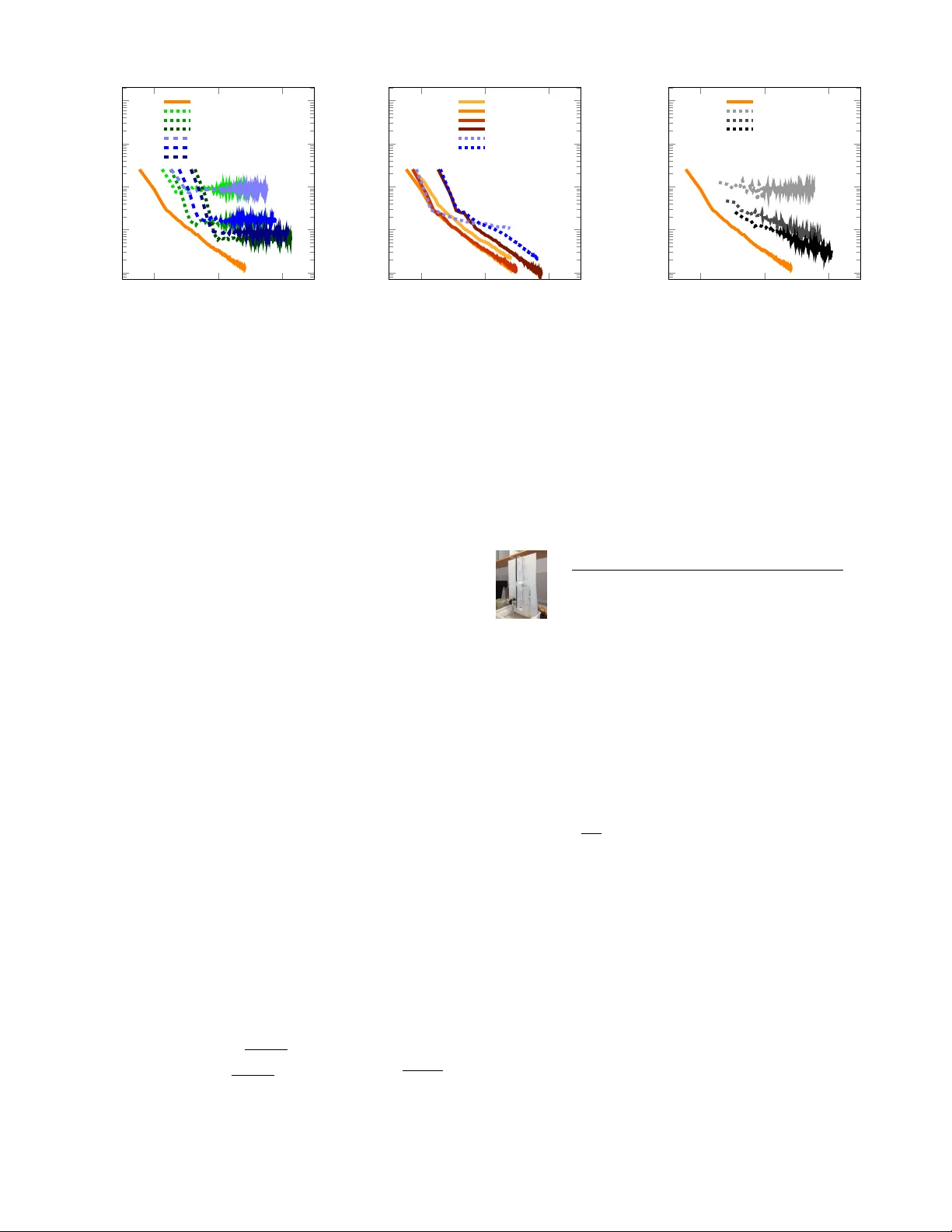
LINDHOLM AND LINDSTEN 2019: LEARNING D YNAMICAL SYSTEMS WITH P AR TICLE STOCHASTIC APPR O XIMA TION EM 1 Learning dynamical systems with particle stochastic approximation EM Andreas Lindholm and Fredrik Lindsten Abstract —W e present the particle stochastic approximation EM (PSAEM) algorithm for lear ning of dynamical systems. The method builds on the EM algorithm, an iterative procedure for maximum likelihood inference in latent variable models. By combining stochastic approximation EM and particle Gibbs with ancestor sampling (PGAS), PSAEM obtains superior com- putational perf ormance and con vergence properties compared to plain particle-smoothing-based approximations of the EM algorithm. PSAEM can be used for plain maximum likelihood inference as well as for empirical Bayes learning of hyper - parameters. Speciﬁcally , the latter point means that existing PGAS implementations easily can be extended with PSAEM to estimate hyperparameters at almost no extra computational cost. W e discuss the con vergence properties of the algorithm, and demonstrate it on several signal processing applications. I . I N T R O D U C T I O N L EARNING of dynamical systems, or state-space models, is central to many classical signal processing problems, such as time-series modeling, ﬁltering and control design. State-space models are also at the core of recent model dev elopments in machine learning, such as Gaussian process state-space models [1], [2], inﬁnite factorial dynamical models [3], [4], and stochastic recurrent neural networks [5, for ex- ample]. A strategy to learn state-space models, independently suggested by [6] and [7], is the use of the Expectation Maxi- mization (EM) [8] method. Originally proposed for maximum likelihood estimation of linear models with Gaussian noise, the strategy can be generalized to the more challenging non-linear and non-Gaussian cases, as well as the empirical Bayes setting. Many contrib utions have been made during the last decade, and this paper takes another step along the path towards a more computationally efﬁcient method with a solid theoretical ground for learning of nonlinear dynamical systems. T o set the notation for this article, we write a gen- eral (discrete-time, non-linear and non-Gaussian) state-space model, or dynamical system, as x t ∼ p θ ( x t | x t − 1 ) , (1a) y t ∼ p θ ( y t | x t ) , (1b) with transition density function p θ ( x t | x t − 1 ) and observ ation density function p θ ( y t | x t ) , parameterized by some unkno wn parameter θ ∈ Θ ⊂ R p . Here, { x t ∈ X ⊂ R m } t =0 , 1 ,... denotes the unobserved state and { y t ∈ Y ⊂ R d } t =1 , 2 ... denotes the observations, and the index t is referred to as ’time’. The initial Andreas Lindholm is with the Department of Information T echnology , Uppsala Univ ersity , Sweden. E-mail: andreas.lindholm@it.uu.se. Fredrik Lindsten is with the Division of Statistics and Machine Learning, Linkping Univ ersity , Sweden. E-mail: fredrik.lindsten@liu.se. state x 0 is distributed according to 1 p ( x 0 ) . W e consider θ as unknown and the focus of this paper is to learn it from recorded data ( y 1 , ..., y T ) , y 1: T . The EM algorithm, which is the strategy we will follow , iterativ ely solves an integration problem and a maximization problem. When using EM for learning state-space models (1), the integral includes the posterior distribution of the unob- served states x 0: T , and possibly also the parameter θ . This distribution is in general analytically intractable, but can be approximated using computational methods such as particle ﬁlters/sequential Monte Carlo (SMC). The combination of EM and SMC, as suggested by [9], [10], [11], has pro vided a principled solution to the challenging problem of learning general state-space models (1), but is unfortunately ‘doubly asymptotic’; to ensure con ver gence, it requires (i) for each iteration of the EM algorithm an inﬁnite number of particles/Monte Carlo samples for approximating the posterior of x 0: T , and (ii) the EM algorithm itself con- ver ges only as its number of iterations goes to inﬁnity . This is a theoretical as well as a practical issue, and we will in this paper e xplore a solution where particle Marko v chain Monte Carlo (PMCMC), rather than plain SMC, is used, which allo ws the two asymptotical con vergences to be ‘entangled’. This will giv e us an algorithm which relies on asymptotics only in one dimension (its number of iterations, not the number of parti- cles), and thereby enjoys a signiﬁcantly reduced computational cost and superior con ver gence properties compared to the predecessors. This overall picture is also brieﬂy summarized in Figure 1. Throughout the paper we assume that the reader is familiar with Markov chain Monte Carlo (MCMC, [12], [13]) as well as particle ﬁlters/SMC [14], [15]. I I . P R O B L E M F O R M U L A T I O N A N D C O N C E P T UA L S O L U T I O N Giv en a batch of observations y 1: T we wish to learn the unknown parameters θ as well as the unobserved states x 0: T of the model (1). For the states x 0: T we are interested in their posterior distrib ution. For the parameters θ , we consider tw o cases: In the frequentistic, or rather Fisherian, setting we are interested in a (possibly regularized) maximum likelihood es- timate b θ . In the Bayesian setting, we assign a prior distribution to the parameters, θ ∼ p η ( θ ) . The prior , in turn, is assumed to be parameterized by some hyperparameter η , which needs to be estimated 2 . Thus, we address both of the following two problems: 1 For notational brevity we assume that the initial density p ( x 0 ) is fully speciﬁed and not parameterized by θ , but the extension to an unknown initial density is straightforward. 2 Hyperparameters can also be set using prior kno wledge. LINDHOLM AND LINDSTEN 2019: LEARNING D YNAMICAL SYSTEMS WITH P AR TICLE STOCHASTIC APPRO XIMA TION EM 2 Solve an integral with respect to p θ k − 1 ( x 0: T | y 1: T ) Solve a maximization problem (depending on the integral) to get θ k k ← k + 1 3 con vergence as k → ∞ (a) EM Approximate the integral by N samples from p θ k − 1 ( x 0: T | y 1: T ) Solve a maximization problem (depending on the N samples) to get θ k k ← k + 1 ! con vergence as k → ∞ and N → ∞ (b) Monte Carlo EM Draw a fe w samples from a Markov k ernel with in variant distribution p θ k − 1 ( x 0: T | y 1: T ) Solve a maximization problem (depending on all past samples) to get θ k k ← k + 1 3 con vergence as k → ∞ (c) SAEM Fig. 1: A brief summary of the different ﬂav ors of Expectation Maximization (EM) methods for maximum likelihood estimation of θ . When it is possible to solve the state inference problem (computing p θ k ( x 0: T | y 1: T ) ) analytically , vanilla EM (a) is the preferred solution. For general models of the form (1)) this is not possible and numerical approximations are required. Monte Carlo EM (b) can be used with a particle smoother (an extension of the particle ﬁlter/SMC) to generate approximate samples from p θ k ( x 0: T | y 1: T ) , which has been proposed independently in the literature several times. Alternati vely , stochastic approximation EM (SAEM, (c)) can be used (whose conver gence properties are superior to Monte Carlo EM), and if the required Markov kernel is built up using the particle ﬁlter in Algorithm 1 we refer to it as PSAEM, the main contribution of this paper . 1) (Fisherian setting) Compute the maximum likelihood estimate of the model parameters, b θ = arg max θ log p θ ( y 1: T ) , where p θ ( y 1: T ) = R p θ ( y 1: T | x 0: T ) p θ ( x 0: T )d x 0: T is the likelihood function. A regularization term, such as k θ k 1 , may also be included in the maximization criterion. 3 2) (Bayesian setting) Compute the posterior distribution of the model parameters p b η ( θ | y 1: T ) , where the h yperparam- eters are estimated using empirical Bayes b η = arg max η log p η ( y 1: T ) , where the marginal likelihood function is p η ( y 1: T ) = R p θ ( y 1: T | x 0: T ) p θ ( x 0: T ) p η ( θ )d θ d x 0: T . These two problems are in fact strongly related, and can be seen as exactly the same problem on a more abstract lev el. In the interest of concreteness we will, ho we ver , distinguish between those two problems, but the computational algorithm that we will propose can be used to address both. The algorithm will compute a Monte Carlo approximation of the posterior distribution over the latent v ariables. Both settings in volv e the computation of a maximum like- lihood estimate; of the model parameters in the ﬁrst case and of the hyperparameters in the second case. A conceptual solution to these problems is giv en by the expectation max- imization (EM, [8]) algorithm. EM is a data augmentation method, meaning that it is based on the notion of a complete data , comprising the observed data as well as the latent (or missing) v ariables. The EM algorithm iterativ ely updates the (hyper-)parameters, and each iteration consists of two steps: (E) Compute the expected value of the complete data log- likelihood for ﬁxed (hyper-)parameters (M) Maximize the Q -function (which will be deﬁned belo w) with respect to the (hyper -)parameters 3 T o avoid too complicated expressions, we do not include the regularization term. From a user’ s perspective, it simply amounts to replace p θ ( y 1: T | x 0: T ) , whenev er it appears, with p θ ( y 1: T | x 0: T ) + λ 1 n k θ k 1 . The observed data is al ways y 1: T , and what differs between the Fisherian and the Bayesian problem is what constitutes the latent v ariables. For the Fisherian problem, the latent variables are x 0: T and we obtain, at iteration k , (E) Let Q Fish k ( θ ) := Z log p θ ( y 1: T , x 0: T ) p θ k − 1 ( x 0: T | y 1: T )d x 0: T , (M) Solve θ k ← arg max θ Q Fish k ( θ ) . (2) Note that the expectation in the (E)-step is w .r .t. the smooth- ing distribution p θ k − 1 ( x 0: T | y 1: T ) parameterized by the previ- ous parameter iterate θ k − 1 . It is well known that iterating (2) giv es a monotone increase of the likelihood p θ k ( y 1: T ) , and θ k will under weak assumptions con ver ge to a stationary point of the likelihood function as k → ∞ (e.g. [16]). For empirical Bayes we obtain similar e xpressions, but the latent variables are both x 0: T and θ . The (E)-step is as (E) Let Q Bay k ( η ) := Z log p η ( y 1: T , x 0: T , θ ) p η k − 1 ( θ , x 0: T | y 1: T )d θ d x 0: T = Z log p η ( θ ) p η k − 1 ( θ | y 1: T )d θ + const. , (M) Solve η k ← arg max η Q Bay k ( η ) , (3) where the second line of (3) follows from the fact that in the factorization of the complete data likelihood, only the prior density p η ( θ ) depends on the hyperparameter η . The M- step remains unchanged. In complete analogy to the Fisherian setting, (3) will also under weak assumptions con ver ge to a stationary point of the mar ginal likelihood as k → ∞ . Both (2) and (3) can be implemented and iterated until con ver gence, as long as the integrals can be computed and the maximization problem solv ed. Howe ver , in most cases— speciﬁcally for the models we consider in this paper—the integrals can not be solved analytically , and the topic for the rest of this paper is essentially to design an ef ﬁcient method for approximating the integrals. The solution will be based on PMCMC [17], but also a stochastic approximation of the Q -function [18] to ensure a computationally efﬁcient solution with good con ver gence properties. Our solution will therefore be more in volv ed than just replacing the integrals in (2) or (3) with vanilla Monte Carlo estimators (Monte Carlo EM). LINDHOLM AND LINDSTEN 2019: LEARNING D YNAMICAL SYSTEMS WITH P AR TICLE STOCHASTIC APPRO XIMA TION EM 3 A short word on notation: we will use subscripts to denote sequences of variables for which we are seeking a maximum, like η k , and brackets for samples of variables for which we are seeking a posterior distrib utions, like x 0: T [ k ] . I I I . R E L AT E D W O R K A N D C O N T R I B U T I O N S The use of EM for learning linear state-space models appears to have been independently suggested by , at least, [6] and [7]. For linear models the state inference problem can be solved exactly using a Kalman ﬁlter , but not for nonlinear models. T o this end, the extended Kalman ﬁlter has been proposed [19], [20], as well as SMC-based solutions [9], [10], [11], leading to a so-called Monte Carlo EM solution. EM is a general strategy for latent variable models, and the standard choice in the application of EM to state-space models is to select the states as the latent variable. It is, howe ver , shown by [21] that if considering the process noise realization (instead of the states) as latent variables, it is possible to introduce stability guarantees for the learned model at the cost of a more inv olved maximization problem. This paper considers the ofﬂine (or batch) problem, but EM can also be applied for online (or streaming data) problems. For the nonlinear online problem, the combination of EM and SMC dates back to at least [22], [23], and recent contributions include [24]. Stochastic approximation EM (SAEM, [18], [25]) can be used to improve the con ver gence properties and reduce the computational cost, compared to Monte Carlo EM. This is particularly true when the Monte Carlo simulation is compu- tationally in v olved, which is the case for SMC-based solutions. In the context of state-space models, SAEM appears to ﬁrst hav e been proposed by [26] and [27], who suggest to combine it with a particle independent Metropolis–Hastings procedure (PIMH, [17]) to infer the latent states. The idea to combine SAEM with particle Gibbs with ancestor sampling (PGAS, [28]), which often has a much lower computational cost, was ﬁrst suggested in a brief conference paper by [29]—the present article is an e xtension of this paper . Since its ﬁrst publication, this method—which we refer to as PSAEM— has found applications in system identiﬁcation [30], [31], causal inference [32], and econometrics [33], to mention a fe w . In this paper , we will study PSAEM more thoroughly , formulate it explicitly for empirical Bayes, present a new theoretical result, and illustrate the method’ s applicability to some contemporary dynamical systems models from the machine learning litera- ture (Gaussian process state-space models [1], [34] and inﬁnite factorial dynamical models [4]). I V . P A RT I C L E S T O C H A S T I C A P P RO X I M A T I O N E M W e will now build up and present the contribution of this paper , the particle stochastic approximation EM (PSAEM) algorithm. The two main components are (i) an MCMC kernel for simulating the latent variables from either p θ ( x 0: T | y 1: T ) or p η ( θ , x 0: T | y 1: T ) , and (ii) a stochastic approximation ver- sion of the EM algorithm (SAEM, [18], [25]), to update the (hyper-)parameter estimate. W e will start with the former (Section IV -A) and thereafter turn to the latter (Section IV -B). A. Sampling the latent variables using PGAS At the core of the EM algorithm is the posterior inference of the latent v ariables, which is needed for the integrals in (2) or (3). For general non-linear or non-Gaussian state-space models these posterior distributions are intractable and we have to use numerical approximations. Much research has been done ov er the past decades on computational algorithms for this problem, and many po werful tools are av ailable. W e will focus on PMCMC [17] methods which we belie ve are particularly well suited for this. PMCMC is a frame work for using particle ﬁlters to construct ef ﬁcient high-dimensional Markov kernels, and we will speciﬁcally make use of the particle Gibbs with ancestor sampling (PGAS) [28]. PGAS has been shown to hav e good empirical performance in many situations (e.g., [35], [36], [4], [37]), but other versions of particle Gibbs could possibly also be employed, such as Particle Gibbs with backward simulation [38], [39] or blocked particle Gibbs [40]. T o start we assume that the parameters to estimate ( θ or η ) are ﬁxed at some v alue, and consider how p θ ( x 0: T | y 1: T ) or p η ( θ , x 0: T | y 1: T ) can be approximated using PGAS. Consider ﬁrst the Fisherian setting. Just like any MCMC method would do, PGAS makes use of an Markov kernel on the space X T +1 with p θ ( x 0: T | y 1: T ) as its unique stationary distribution. This k ernel is then applied iterati vely , and if certain ergodic- ity assumptions hold, this procedure will eventually produce samples from p θ ( x 0: T | y 1: T ) . With PGAS this Markov kernel is constructed using a particle ﬁlter , or more precisely a conditional particle ﬁlter with ancestor sampling , gi ven in Algorithm 1. One execution of the entire Algorithm 1 corre- sponds to one iteration of the Markov kernel. The conditional particle ﬁlter resembles a standard particle ﬁlter with N − 1 particles, with the addition that there is also a conditional particle trajectory (for con venience numbered N , line 2 and 8) which is speciﬁed a priori. In the resampling step (line 5), this conditional trajectory can be replicated, but nev er discarded. At the end, one single trajectory is extracted, which will be used as conditional trajectory in a later iteration. The ancestor sampling (line 7) assigns ancestors to the conditional trajectory , similar to resampling b ut ‘backwards’ in time and only for the conditional trajectory . W e refer to [28] for further details. Algorithm 1 is formulated in its ‘bootstrap’ v ersion, but a more general SMC formulation is also possible, see [28]. Formally we let Algorithm 1 deﬁne a Markov kernel Π θ on the space of state trajectories X T +1 giv en by Π θ ( x 0 0: T , B ) = E [ 1 ( x ? 0: T ∈ B )] (4) where the expectation is w .r .t. the random variables used in Algorithm 1. The Markov kernel constructed by Algorithm 1 takes a state trajectory x 0: T [ j − 1] = x 0 0: T ∈ X T +1 as input and outputs another state trajectory x 0: T [ j ] = x ? 0: T ∈ X T +1 . Put differently , a sample x 0: T [ j ] ∼ Π θ ( x 0: T [ j − 1] , · ) can be gen- erated by ex ecuting Algorithm 1 with ﬁxed θ and x 0: T [ j − 1] as input reference trajectory . If this is iterated, an MCMC procedure on the space X T +1 is obtained, and the trajectories x 0: T [0] , x 0: T [1] , x 0: T [2] , . . . , will eventually be samples from the sought smoothing distribution p θ ( x 0: T | y 1: T ) . MCMC methods like this, which uses Mark ov k ernels based on particle ﬁlters, are called PMCMC. LINDHOLM AND LINDSTEN 2019: LEARNING D YNAMICAL SYSTEMS WITH P AR TICLE STOCHASTIC APPRO XIMA TION EM 4 Algorithm 1 Mark ov kernel Π θ ( x 0 0: T , x ? 0: T ) Input: Conditional trajectory x 0 0: T , parameter θ . Output: Trajectory x ? 0: T . 1: Draw x i 0 ∼ p ( x 0 ) , i = 1 , . . . , N − 1 . 2: Set x N 0 ← x 0 0 . 3: Set w i 0 ← 1 , i = 1 , . . . , N . 4: for t = 1 , 2 , . . . , T do 5: Draw a i t with Pr( a i t = j ) ∝ w j t − 1 for i = 1 , . . . , N − 1 . 6: Draw x i t ∼ p θ ( x t | x a i t t − 1 ) for i = 1 , . . . , N − 1 . 7: Draw a N t with Pr( a N t = j ) ∝ w j t − 1 p θ ( x 0 t | x j t − 1 ) . 8: Set x N t ← x 0 t . 9: Set w i t ← p θ ( y t | x i t ) for i = 1 , . . . , N . 10: end for 11: Draw I with Pr( I = i ) ∝ w i T . 12: Set x ? T = x I T . 13: for t = T − 1 , T − 2 , . . . , 0 do 14: Set I ← a I t +1 . 15: Set x ? t ← x I t . 16: end for It is far from obvious that Π θ admits p θ ( x 0: T | y 1: T ) as its stationary distribution. Howe ver , its properties (as well as those of its older sibling presented by [17]) have been extensi vely studied, see for e xample [17], [41], [28], [42], [43], [44]. The main results are: (i) p θ ( x 0: T | y 1: T ) is a stationary distribution of Π θ , and (ii) Π θ is uniformly geometrically ergodic in x 0: T for any N ≥ 2 and any θ ∈ Θ under upper boundedness conditions on w i t in Algorithm 1. W e summarize this PMCMC procedure to infer p θ ( x 0: T | y 1: T ) in Algorithm 2 (still assuming θ is ﬁx ed). Algorithm 2 Sampling p θ ( x 0: T | y 1: T ) (Fisherian, ﬁx ed θ ) 1: Initialize x 0: T [0] arbitrarily , e.g., by running a standard particle ﬁlter targeting p θ ( x 0: T | y 1: T ) . 2: for j = 1 , 2 , . . . , J do 3: Sample x 0: T [ j ] ∼ Π θ ( x 0: T [ j − 1] , · ) (run Alg. 1 once) 4: end for So far we hav e only considered the Fisherian setting, in which the latent variables only comprise the state trajectory . For the Bayesian setting we assume that η (instead of θ ) is ﬁxed, and we see from (3) that we have to compute the model parameter posterior distribution p η ( θ | y 1: T ) . W e will do this by splitting the simulation problem into two steps, one in which we sample x 0: T conditionally on θ (and y 1: T ) and one in which we sample θ conditionally on x 0: T (and y 1: T ). The ﬁrst step, sampling x 0: T conditionally on θ , is equiv alent to the problem discussed for the Fisherian setting, and we can use the Markov kernel Π θ Algorithm 1. For the second step, sampling θ conditionally on x 0: T , exact solutions are often possible, leading to Gibbs sampling. Otherwise, methods like Hastings- within-Gibbs (see, for instance, [13, Section 2.4]) are possible. The particular choice depends on the actual model, and we will later illustrate it by an example. Let the Markov kernel used to simulate θ be denoted by Π η ,x 0: T ( θ 0 , · ) . Most of the previously referenced literature on properties for Π θ cov ers also the setting of a joint kernel for θ, x 0: T . The resulting MCMC procedure used in the Bayesian setting (still assuming a ﬁxed value for η ) is summarized in Algorithm 3, and conv erges (in the same sense as Algorithm 2) to p η ( θ , x 0: T | y 1: T ) . Algorithm 3 Sampling p η ( θ , x 0: T | y 1: T ) (Bayesian, ﬁx ed η ) 1: Initialize θ [0] and x 0: T [0] arbitrarily . F or the latter e.g., by a particle ﬁlter targeting p θ [0] ( x 0: T | y 1: T ) 2: for j = 1 , 2 , . . . do 3: Sample x 0: T [ j ] ∼ Π θ [ j − 1] ( x 0: T [ j − 1] , · ) (run Alg. 1 once) 4: Sample θ [ j ] ∼ Π η,x 0: T [ j ] ( θ [ j − 1] , · ) 5: end for B. Combining PGAS and EM W e hav e so far assumed that the (hyper-)parameters are ﬁx. The objective in this paper is, howe ver , to learn those, and we will for this purpose use a stochastic approximation version of the EM algorithm. 1) A naive solution using EM and PMCMC: The problem with the preliminary EM solutions outlined in (2) and (3), respectiv ely , is the analytically intractable integrals in their Q - functions. A ﬁrst idea would be to replace the integrals with sums over J Monte Carlo samples. For the Fisherian setting, this means replacing the (E)-step of (2) with a simulation (Si) step as follo ws: (Si) ( Draw { x 0: T [ j ] } J j =1 ∼ p θ k − 1 ( x 0: T | y 1: T ) and let b Q Fish k ( θ ) := 1 J P J j =1 log p θ ( y 1: T , x 0: T [ j ]) . (M) Solve θ k ← arg max θ b Q Fish k ( θ ) . (5) Note that this is our initial EM scheme (2), but with the analytically intractable inte gral ov er log p θ ( y 1: T , x 0: T ) approx- imated by a sum. This algorithm is commonly referred to as Monte Carlo EM [45] or , if J = 1 , stochastic EM [46]. T o draw the samples in the (Si)-step we can use PGAS from Section IV -A, which w ould give Algorithm 4. Algorithm 4 Monte Carlo EM for the Fisherian problem 1: Initialize θ 0 2: for k = 1 , 2 , . . . do 3: Run Alg. 2 with θ k − 1 ‘until conv ergence’, get { x 0: T [ j ] } J j =1 4: Solve θ k ← arg max θ 1 J P J j =1 log p θ ( y 1: T , x 0: T [ j ]) 5: end for A similar algorithm could be devised for the Bayesian setting. Even though Algorithm 4 might look promising, there are two issues with this solution: (i) T o guarantee that Algorithm 2 has con ver ged to its stationary distribution, we cannot bound its number of iterations at line 3. (ii) For the sum in (5)/line 4 to con ver ge to the integral it approximates, we must let J → ∞ . Indeed, these tw o issues are related. W e basically need to allo w J → ∞ to ensure conv ergence, whilst the con ver gence of the EM iteration happens as k → ∞ . This is not desirable since it, intuitively , gives a computational complexity of “ ∞ × ∞ ”; see further [47]. Existing methods based on various types of particle smoothing for approximating the integral with respect to p θ ( x 0: T | y 1: T ) , for instance [10], [11], suffer from the same issues. Indeed, these methods are (SMC-based) instances of Monte Carlo EM. W e will now ﬁrst address issue (ii) with stochastic approxi- mation EM, and thereafter handle issue (i) by ‘entangling’ the con ver gence of Algorithm 2 ( J → ∞ ) with the con v ergence of the EM algorithm ( k → ∞ ). LINDHOLM AND LINDSTEN 2019: LEARNING D YNAMICAL SYSTEMS WITH P AR TICLE STOCHASTIC APPRO XIMA TION EM 5 2) SAEM: Handling sample appr oximations within EM: Stochastic approximation, as introduced by [48], is an a ver - aging procedure to solve a (deterministic) equation which can only be ev aluated through noisy (stochastic) observ ations. In stochastic approximation a step length γ k ∈ [0 , 1] is used, which has to fulﬁll ∞ X k =1 γ k = ∞ , ∞ X k =1 γ 2 k < ∞ , γ 1 = 1 . (6) Follo wing [18], the SAEM algorithm can be introduced by making a stochastic approximation of the Q -function. In SAEM, we transform Monte Carlo EM (5) by introducing a stochastic approximation (SA)-step. For simplicity we only use one sample ( J = 1 ) in the simulation (Si)-step, but in practice it can be fa vorable to use a small batch of samples. For iteration k this becomes (Si) Draw x 0: T [ k ] ∼ p θ k − 1 ( x 0: T | y 1: T ) . (SA) Let Q Fish k ( θ ) ← (1 − γ k ) Q Fish k − 1 ( θ ) + γ k log p θ ( y 1: T , x 0: T [ k ]) . (M) Solve θ k ← arg max θ Q Fish k ( θ ) . (7) T o intuitively understand the stochastic approximation, let us ﬁrst ignore the (M)-step and assume γ k = 1 k . In such a case, the (SA)-step would simply be online averag- ing, equi valent to Q Fish k ( θ ) = 1 k P k ` =1 log p θ ( y 1: T , x 0: T [ ` ]) , where x 0: T [ ` ] ∼ p θ ( x 0: T | y 1: T ) , which conv erges to R log p θ ( y 1: T , x 0: T ) p θ ( x 0: T | y 1: T )d x 0: T when k → ∞ by the law of large numbers. The introduction of the (M) step complicates the picture, but assuming that θ k will e ventually con ver ge to a stationary point, the inﬂuence from the transient phase will v anish as k → ∞ , and the averaging argument can still be applied. In Section V we discuss the con ver gence properties in detail. Before that, in Section IV -C, we will consider the important special case of exponential family models, for which the (SA) step reduces to a con venient recursiv e update of sufﬁcient statistics. W ith (7) in place, we can make stronger theoretical claims (ev en though we are using only a single sample, J = 1 , from p θ k − 1 ( x 0: T | y 1: T ) , at each iteration!) thanks to the use of stochastic approximation [18]. Howe ver , for the problem under study it is still of limited practical use since we cannot generate samples from p θ k − 1 ( x 0: T | y 1: T ) by other means than using Algorithm 2 with an inﬁnite number of iterations (in order to ensure that it has conv erged). Thus, our ﬁnal step is to use the method studied by [25] to combine SAEM with an MCMC procedure in a more intricate way than (7). 3) PSAEM: Combining SAEM with PGAS: As suggested and analyzed by [25], the draw from p θ k − 1 ( x 0: T | y 1: T ) in (7) can be replaced with a draw from a Marko v kernel which has p θ k − 1 ( x 0: T | y 1: T ) as its inv ariant distribution. As discussed, this is exactly what Π θ from Algorithm 1 is, and we can thus assemble (Si) Draw x 0: T [ k ] ∼ Π θ k − 1 ( x 0: T [ k − 1] , · ) (that is, run Algorithm 1 once ) . (SA) Let Q Fish k ( θ ) ← (1 − γ k ) Q Fish k − 1 ( θ ) + γ k log p θ ( y 1: T , x 0: T [ k ]) . (M) Solve θ k ← arg max θ Q Fish k ( θ ) . (8) Note that we do not make use of Algorithm 2 anymore, but only Algorithm 1. This means that we do not run the Markov kernel “until conv ergence” at each iteration, but it will (intuitively speaking) con ver ge in parallel with the SAEM iterations indexed with k . W e summarize and present this as Algorithms 5 and 6. Algorithm 5 PSAEM for the Fisherian setting 1: Initialize x 0: T [0] , θ 0 2: for k = 1 , 2 , . . . do 3: Run Alg. 1 cond. on x 0: T [ k − 1] and θ k − 1 to sample x 0: T [ k ] 4: Q Fish k ( θ ) ← (1 − γ k ) Q Fish k − 1 ( θ ) + γ k log p θ ( y 1: T , x 0: T [ k ]) 5: Solve and update parameters θ k ← arg max θ Q Fish k ( θ ) 6: end for Algorithm 6 PSAEM for the Bayesian setting 1: Initialize x 0: T [0] , θ [0] , η 0 2: for k = 1 , 2 , . . . do 3: Run Alg. 1 cond. on x 0: T [ k - 1] and θ [ k - 1] to sample x 0: T [ k ] 4: Sample θ [ k ] ∼ Π η k − 1 ,x 0: T [ k ] ( θ [ k − 1] , · ) 5: Update Q Bay k ( η ) ← (1 − γ k ) Q Bay k − 1 ( η ) + γ k log p η ( θ [ k ]) 6: Solve and update hyperparameters η k ← arg max η Q Bay k ( η ) 7: end for W e ha ve now obtained an algorithm which only relies on asymptotics as k → ∞ , by ‘entangling’ the con ver gence of PGAS with the con vergence of SAEM. As we will see in Sec- tion V, con ver gence can be shown under certain assumptions. W e will no w consider the important special case of models (1) in the exponential family , for which the recursively deﬁned function Q k reduces to a much simpler expression. C. PSAEM for e xponential family models Studying Algorithm 5 or 6, one may expect the compu- tational cost of all computations in volving the Q -function to increase as k → ∞ , since Q k is deﬁned as a sum with k terms, each a function of a past sample of x 0: T . This is, ho wev er , not the case if the model belongs to the exponential family , which is an important special case discussed belo w . When we write “the model belongs to the exponential family”, we mean that the joint distribution for the latent and observed variables, p θ ( x 0: T , y 1: T ) or p η ( θ , x 0: T , y 1: T ) , belongs to the exponential family with θ or η as its parameter, respectiv ely . For the Fisherian case, this is fulﬁlled if both equations in (1) can, with some choice of S x : X × X → R ` , ψ x : Θ → R , φ x : Θ → R ` (for some ` ), and similarly for some S y , ψ y , φ y , be written as p θ ( x t | x t − 1 ) θ ∝ exp {− ψ x ( θ ) + h S x ( x t − 1 , x t ) , φ x ( θ ) i} , (9a) p θ ( y t | x t ) θ ∝ exp {− ψ y ( θ ) + h S y ( x t , y t ) , φ y ( θ ) i} . (9b) Here, θ ∝ reads “proportional (with respect to θ ) to” and h· , ·i is an inner product. The subscripts ( x , y and θ ) do not denote dependencies in this context, but are only names. For the Bayesian case, the requirements are weaker , and it is enough that the prior distribution for θ belongs to the exponential family , p η ( θ ) η ∝ exp {− ψ θ ( η ) + h S θ ( θ ) , φ θ ( η ) i} . (10) LINDHOLM AND LINDSTEN 2019: LEARNING D YNAMICAL SYSTEMS WITH P AR TICLE STOCHASTIC APPRO XIMA TION EM 6 W e will no w see ho w the Q -function from the (SA)-step simpliﬁes for models which can be written on one of these forms. First consider the Fisherian case. Using the Markovian structure of (1), we can write log p θ ( y 1: T , x 0: T ) = T X t =1 log p θ ( y t | x t ) + log p θ ( x t | x t − 1 ) + const. = − ψ ( θ ) + h S ( x 0: T , y 1: T ) , φ ( θ ) i + const. (11) where ψ ( θ ) = T { ψ x ( θ ) + ψ y ( θ ) } , S ( x 0: T , y 1: T ) = T X t =1  S x ( x t − 1 , x t ) S y ( x t , y t )  , φ ( θ ) =  φ x ( θ ) φ y ( θ )  . Here we have used the fact that the initial distribution p ( x 0 ) is independent of θ (for notational simplicity). It follows that Q Fish k ( θ ) = − ψ ( θ ) + h S k , φ ( θ ) i + constant , (12a) where S k = (1 − γ k ) S k − 1 + γ k S ( x 0: T [ k ] , y 1: T ) . (12b) Note that this is a non-recursiv e deﬁnition of Q Fish k ( θ ) , but instead recursiv e in S k . From an algorithmic point of view , this means that we can compute and store S k as (12b), and solve the maximization problem for (12a) instead of the more intricate and computationally challenging (8). In fact, the maximizing argument to (12a) can be expressed on closed form in man y cases. Analogously the Bayesian case is obtained as, Q Bay k ( η ) = − ψ θ ( η ) + h S k , φ θ ( η ) i + constant . (13a) where S k = (1 − γ k ) S k − 1 + γ k S θ ( θ [ k ]) . (13b) W e summarize in Algorithms 7 and 8. Algorithm 7 PSAEM for exponential f amily models, Fisherian 1: Initialize x 0: T [0] and θ 0 2: for k = 1 , 2 , . . . do 3: Run Algorithm 1 conditional on x 0: T [ k − 1] and θ k − 1 to sample x 0: T [ k ] 4: Update sufﬁcient statistics S k according to (12b) 5: Solve and update parameters θ k ← arg max θ Q Fish k ( θ ) using (12a) 6: end for Algorithm 8 PSAEM for exponential f amily models, Bayesian 1: Initialize x 0: T [0] , θ [0] and η 0 2: for k = 1 , 2 , . . . do 3: Run Algorithm 1 conditional on x 0: T [ k − 1] and θ [ k − 1] to sample x 0: T [ k ] 4: Sample θ [ k ] ∼ Π η k − 1 ,x 0: T [ k ] ( θ [ k − 1] , · ) 5: Update sufﬁcient statistics S k according to (13b) 6: Solve and update hyperparameters η k ← arg max η Q Bay k ( η ) using (13a) 7: end for V . C O N V E R G E N C E The con ver gence of SAEM and its extensions, including MCMC-based implementations, has receiv ed a lot of attention [18], [25], [49], [27]. In Section V -A we present a basic con- ver gence result for PSAEM. This is essentially an application of [25, Theorem 1], howe ver , we also add a missing piece regarding the continuity of the PGAS Markov kernel. This will under certain (strong) assumptions on X and the model (1) imply conv ergence of PSAEM as k → ∞ (with ﬁnite N ≥ 2 ﬁxed in Algorithm 1). Some of these conditions could possibly be weakened by using the algorithmic modiﬁcations proposed by [27], but we do not pursue this further here. W e will also, in Section V -B, discuss some practical considerations regarding the choice of N and γ k . In the presentation belo w we write k f k ∞ = sup x | f ( x ) | for the supremum norm of function f and Π f ( x ) = R Π( x, dx 0 ) f ( x 0 ) for the Markov kernel Π acting on f . A. Theor etical r esults W e will for bre vity present this section in the Fisherian setting. By considering { x 0: T , θ } as the latent variables instead of x 0: T , the results are applicable also to the Bayesian setting. Con ver gence of the SAEM algorithm has only been estab- lished for models in the exponential family . In addition to the requirements on the step size sequence in (6), the essence of the assumptions used by [25] are: (A1) The parameter space Θ is an open subset of R p . The model belongs to the exponential family , and the log- likelihood function and its components φ, ψ and S are sufﬁciently smooth, dif ferentiable and integrable. (A2) A unique solution to the maximization problem in the (M)-step exists, and that mapping from S k to θ k is sufﬁciently differentiable. (A3) X is compact and S is continuous on X . (A4) The Markov kernel Π θ for sampling x 0: T is uniformly ergodic uniformly in θ . Furthermore, Π θ is Lipschitz continuous w .r .t. θ uniformly in x 0: T . Remark: For more precise statements of the actual assump- tions under which we prove con ver gence of PSAEM, see Appendix A. Under such assumptions [25] show that SAEM con ver ges to a stationary point of the likelihood surface. Assumption (A1)- (A3) deﬁne the class of models (1) for which con ver gence is prov en. The compactness assumption on X is strong, and ensures that S k cannot di ver ge, b ut is not strictly necessary . The more general case is, ho we ver , far from tri vial, see [18, Section 5], [49] and [27]. Assumption (A4) puts requirements (uniform ergodicity and Lipschitz continuity) on the MCMC kernel that is used, which is PGAS in our case. Uniform ergodicity has been shown for PGAS under a boundedness assumption on the weights of the conditional particle ﬁlter [28, Theorem 3]. In Appendix A we extend this result to hold uniformly in θ under assumption (A5), stated below . What has not previously been shown, though, is Lipschitz continuity of the PGAS Marko v kernel. This property is establish belo w under the follo wing additional assumption. LINDHOLM AND LINDSTEN 2019: LEARNING D YNAMICAL SYSTEMS WITH P AR TICLE STOCHASTIC APPRO XIMA TION EM 7 (A5) There e xists constants L 1 , L 2 < ∞ , δ 1 , δ 2 > 0 and κ 1 , κ 2 < ∞ , independent of x t − 1 , x t , θ , such that, for all x t − 1 , x t ∈ X and all t = 1 , . . . , T , a) Lipschitz continuity of tr ansition and likelihood den- sities: For all θ, e θ ∈ Θ , | p θ ( x t | x t − 1 ) − p e θ ( x t | x t − 1 ) | ≤ L 1 k θ − e θ k , | p θ ( y t | x t ) − p e θ ( y t | x t ) | ≤ L 2 k θ − e θ k . b) Str ong mixing: F or all θ ∈ Θ , δ 1 ≤ p θ ( x t | x t − 1 ) ≤ κ 1 and δ 2 ≤ p θ ( y t | x t ) ≤ κ 2 . Remark: The lower bound on the state transition and likeli- hood functions in (A5b), commonly referred to as the str ong mixing condition , are indeed strong but have traditionally been used for establishing many theoretical results on SMC, see for instance [50]. Furthermore, this assumption essentially boils down to compactness of X , which is assumed in (A3) already . The strong mixing condition has been weakened for some results [51], [52], and could possibly be e xtended further . Theorem 1 (Lipschitz continuity of PGAS) . Assume (A3) and (A5) and let Π θ denote the PGAS Markov kernel (4) . Then ther e exists a constant C < ∞ such that for any bounded function f : X T +1 → R , it holds that for all θ, e θ ∈ Θ , k Π θ f − Π e θ f k ∞ ≤ C k f k ∞ k θ − e θ k . Pr oof. See Appendix B. W e may no w piece all results together into the main theorem of this section, which establishes the con vergence of PSAEM. Theorem 2 (Con vergence of PSAEM) . Assume (A1)-(A3); see pr ecise statements in Appendix A. Additionally , assume (A5) and let θ k be computed by Algorithm 7. Then, with pr obability 1, lim k →∞ d ( θ k , L ) = 0 , where d ( θ , L ) denotes the distance fr om θ to the set L = { θ ∈ Θ : ∂ ∂ θ p θ ( y 1: T ) = 0 } . Pr oof. The proof, together with precise statements of the assumptions, is given in Appendix A. The big picture is that Theorem 1 (together with existing ergodicity results) implies (A4), and therefore Theorem 2 follows from [25, Theorem 1]. B. Practical considerations Even though Theorem 2 gi ves a reassuring theoretical foundation for using PSAEM, it does not gi ve any practical advice on some of the (fe w) tuning parameters a vailable: the choice of step length { γ k } ∞ k =1 or the number of particles N in Algorithm 1. A common choice for step length is γ k = k − α , and the requirements (6) are fulﬁlled for any α ∈ ( 1 2 , 1] . In our experience, it is often advisable to choose α < 1 , perhaps α = 0 . 7 , not to constrain the steps too much. Even though not necessary , the initial con ver gence speed can sometimes be improv ed by setting some initial step lengths to constant 1 , before starting the sequence of decreasing step lengths. For N , we hav e to make a balance between a well mixing Markov kernel (large N ) and the computational load (small N ). Let K denote the number of iterations of PSAEM, and assume that the computational budget a vailable is such that the product K N is limited. In such a situation, the general advice would be to take N ‘small’ and K ‘large’. Howe ver , if N is too small, the Markov kernel will not mix well, affecting the con ver gence speed. T o monitor the mixing, the ov erlap between two consecutiv e state trajectories x 0: T [ k − 1] and x 0: T [ k ] could be computed, and if it exceeds a certain threshold, say 90% , a warning could be raised that the mixing is not suf ﬁcient and N should be increased. V I . E X P E R I M E N T S A N D A P P L I C AT I O N S W e will in this section ﬁrst (Section VI-A) illustrate the behavior of PSAEM on a small toy example (where the maxi- mum likelihood estimate can be found exactly), and study the advantage over a standard Monte Carlo EM implementation for the same problem. W e will thereafter turn to three dif ferent applications, namely parameter estimation in a non-linear state-space model (the Fisherian setting, Section VI-B), and hyperparameter estimation (Bayesian setting) in inﬁnite facto- rial dynamical models (Section VI-C) and Gaussian process state-space models (Section VI-D), respectively . Full details for all e xamples are found in Appendix C. A. Linear Gaussian state-space model W e consider T = 300 data points from the model x t +1 = θ x t + w t , w t ∼ N (0 , 1) , (14a) y t = x t + e t , e t ∼ N (0 , 0 . 3) , (14b) with θ ∈ ( − 1 , 1) . W e apply PSAEM and four alternativ e methods. A close relativ e to PSAEM, namely PIMH-SAEM (using particle independent Metropolis–Hastings instead of PGAS; [27], [53]), is applied. W e also use two dif ferent Monte Carlo EM solutions (5), one using the forward ﬁlter backward simulator (FFBSi) smoother 4 [10], [54] and one using the particle-based rapid incremental (PaRIS) smoother [55]. Com- pared to FFBSi, the PaRIS smoother has the computational advantage that it approximates not the entire distribution p θ k ( x 0: T | y 1: T ) , but only p θ k ( x t , x t +1 | y 1: T ) , which in fact is sufﬁcient for the Fisherian problem. In fact, PaRIS is an online smoothing algorithm so it can also be combined with online- EM as proposed by [24]. The online-EM method solves indeed also the (challenging) online problem, and is included in the comparison. W e iterate each method 1 000 times, and study the con ver gence to the true maximum lik elihood estimate (which is av ailable exactly in this toy model). For the online-EM algorithm we loop ov er the T = 300 data points 1 000 times (note that this method makes one parameter update per single time step). All methods are applied with different numbers of particles N . In Figure 2, the ev olution of the absolute error is shown as a function of computational time on the same standard desktop computer with comparable implementations, av eraged ov er 200 realizations of each algorithm. Note that PSAEM 4 This is similar to the method proposed by [11], but it uses a more efﬁcient smoother . LINDHOLM AND LINDSTEN 2019: LEARNING D YNAMICAL SYSTEMS WITH P AR TICLE STOCHASTIC APPRO XIMA TION EM 8 10 − 2 10 0 10 2 10 − 3 10 − 2 10 − 1 10 0 10 1 Computational time Absolute error | θ k − b θ ML | PSAEM, N = 10 Monte Carlo EM: FFBSi, N = 3 Monte Carlo EM: FFBSi, N = 10 Monte Carlo EM: FFBSi, N = 50 Monte Carlo EM: PaRIS, N = 3 Monte Carlo EM: PaRIS, N = 10 Monte Carlo EM: PaRIS, N = 50 (a) Besides faster conver gence (in terms of computational time), PSAEM does not suffer from the bias present in Monte Carlo EM. The bias is caused by the ﬁnite number of samples in the integral (5), and the bias v anishes only as N → ∞ , in contrast to PSAEM for which k → ∞ is enough. 10 − 2 10 0 10 2 10 − 3 10 − 2 10 − 1 10 0 10 1 Computational time PSAEM, N = 3 PSAEM, N = 10 PSAEM, N = 100 PSAEM, N = 1000 PIMH-SAEM, N = 100 PIMH-SAEM, N = 1000 (b) The optimal N for PSAEM in this problem appears to be in the range 10–100; smaller N causes poor mixing and slower con ver gence; larger N increases computational cost without improving mixing. PIMH-SAEM with N = 100 struggles because of poor mixing, whereas N = 1000 mixes better at a higher computa- tional cost. 10 − 2 10 0 10 2 10 − 3 10 − 2 10 − 1 10 0 10 1 Computational time PSAEM, N = 10 PaRIS + online-EM, N = 3 PaRIS + online-EM, N = 10 PaRIS + online-EM, N = 50 (c) The conver gence of online-EM with the PaRIS smoother is theoretically not fully un- derstood, but appears for N = 3 to suffer from a similar bias as Monte Carlo EM. For this example it appears to conver ge with larger N , howe ver at a signiﬁcantly higher computational cost than PSAEM. Fig. 2: Estimation of θ in (14) with ﬁv e different methods; the proposed PSAEM, PIMH-SAEM (similar to PSAEM, b ut with a PIMH Markov kernel instead of PGAS), two Monte Carlo EM implementations (using the FFBSi and PaRIS smoother , respectively) and online-EM with the PaRIS smoother . The methods are run with various number of particles N , cf. the discussion on N in Section V -B. Their average evolution of the absolute error | θ k − b θ ML | (over 200 runs), where b θ ML is the exact maximum likelihood estimate, is shown as a function of the wall clock time. All methods are run for 1 000 iterations, and there is a linear relationship between k and computational time for all methods. and PIMH-SAEM con v erge as k → ∞ (for ﬁxed N ), whereas Monte Carlo EM has a non-v anishing bias which only decreases as N → ∞ . In other w ords, k → ∞ is not sufﬁcient for conv ergence in Monte Carlo EM. Comparing PSAEM and PIMH-SAEM, the latter requires a signiﬁcantly larger number of particles than PSAEM, and has therefore a higher computational cost. This difference is likely to be ev en more pronounced for larger values of T , due to superior scaling properties of PGAS compared to PIMH. B. Cascaded water tanks W e consider the benchmark problem of learning a model for a cascaded water tank system, using the data presented by 5 [56]. A training and a test data set of input-output data samples { u t , y t } , each with T = 1024 data points, are provided. The data is recorded from an experimental setup where water is pumped into an upper water tank, from which it ﬂo ws through a small opening into a lower water tank, and from there through another small opening into a basin. During the data collection, the tanks occasionally overﬂo wed, and the excess water from the upper tank partially ﬂo wed into the lower tank. Only the pump voltage (input) and the water le vel in the lower tank (output) is measured each T s = 4 second, and the problem is to predict the water le vel in the lo wer tank giv en only the pump voltage. A physically motiv ated discrete-time nonlinear state-space model (partly adopted from [57]) is x u t +1 =10 ∧ x u t + T s ( − k 1 p 10 ∧ x u t − k 2 { 10 ∧ x u t } + k 5 u t ) + w u t x l t +1 =10 ∧ x l t + T s ( k 1 p 10 ∧ x u t + k 2 { 10 ∧ x u t } − k 3 q 10 ∧ x l t − k 4 { 10 ∧ x l t } + k 6 { ( x u t − 10) ∨ 0 } ) + w l t y t =10 ∧ x l t + e t , (15) 5 See also http://www .nonlinearbenchmark.or g Model Simulation (test data) Initial model to PSAEM 2.85 Estimated with PSAEM 0.29 [58] 0.34 T ABLE I: The cascaded water tank setup and modeling results. W e initialize the 9 unknown parameters with an ad-hoc educated guess (top ro w), and then optimize them with PSAEM (middle ro w). W e also include the best performing result previously published (last ro w). The ﬁgure of merit is root- mean-squared error for simulation on the test data. where the states x u t ∈ R and x l t ∈ R are the water lev els plus the inﬂow in the upper and lower tank, respectiv ely . The parameters k 1 , k 2 , k 3 , k 4 , k 5 represent unknown physical quantities, such as tank and hole diameters, ﬂow constants, pump efﬁcienc y , etc. Each tank has height 10 (in the scale of the sensor), and k 6 and 10 ∧ ( . . . ) is moti vated by the overﬂo w ev ents. The initial lev el of the upper water tank is modeled as x u 0 ∼ N ( ξ 0 , √ 0 . 1) , with ξ 0 unknown. Furthermore, w 1 t , w 2 t and e t are assumed to be zero mean white Gaussian noise with unknown variances σ 2 w and σ 2 e , respectiv ely . All in all, the un- known parameters are θ = { k 1 , k 2 , k 3 , k 4 , k 5 , k 6 , σ 2 e , σ 2 w , ξ 0 } . The model belongs to the e xponential f amily , and we can thus apply PSAEM as presented in Algorithm 7 to ﬁnd a maximum likelihood estimate of θ . W e initialize θ randomly around physically reasonable values, and run PSAEM for 50 iterations with N = 100 (taking a few seconds on a standard desktop computer). The obtained results are reported in T able I together with the best performing result pre viously published (to the best of our knowledge). Many previously published methods use a more data-driven approach, but the relativ ely small amount of data makes the encoding of ph ysical knowledge important, as done here by (15) and PSAEM. LINDHOLM AND LINDSTEN 2019: LEARNING D YNAMICAL SYSTEMS WITH P AR TICLE STOCHASTIC APPRO XIMA TION EM 9 Algorithm 9 PSAEM for inﬁnite factorial dynamical models: the cocktail party example 1: for k = 0 to K do 2: Update the state dimensionality (number of speakers) M + using slice sampling. 3: Sample a state trajectory using PGAS. 4: Gibbs update of the transition probabilities { b m } M + m =1 for each speaker . 5: S k ← (1 − γ k ) S k − 1 + γ k S ( { b m } M + m =1 ) , with S being sufﬁcient statistics for the Beta distribution. 6: η k ← arg max η Q Bay k ( η ) = arg max η h S k , φ ( η ) i − ψ ( η ) . 7: Gibbs update of noise variance parameters. 8: end for C. Hyperparameters in inﬁnite factorial dynamical models The inﬁnite factorial dynamical model (iFDM, [4]) is a Bayesian non-parametric model for separation of aggregated time-series into independent sources. By using a Markov Indian buf fet process, the number of sources (dimensionality of the hidden state) does not hav e to be upper bounded a priori. Each source is modeled as a (discrete or continuous) Markov chain which e volves independently of the other . T o solve the inference problem, i.e., performing the actual source separation, PGAS has proven useful [4]. There is, howe ver , a multitude of hyperparameters in this Bayesian setting, and we demonstrate how the procedure by [4] easily can be extended with PSAEM to automatically estimate hyperparameters on- the-ﬂy , reducing the need for extensiv e manual tuning. W e will consider the cocktail party problem originating from [3], to which iFDM has been applied [4, Section 4]. The voices from 15 different speakers is aggregated into a T = 1085 long sequence, together with some noise, and the problem is to jointly infer (i) the number of speakers (dimension of x t ), (ii) when each speaker is talking (the trajectory x t ) and (iii) the dynamics of each speaker (how prone s/he is to talk). Each speaker is modeled as a Markov chain with two states, ‘talking’ or ‘quiet’, and the posterior distribution over its transition probabilities is inferred indi- vidually for each speaker . The Beta distribution is used as prior for these probabilities, and the hyperparameters for the Beta distrib ution are manually chosen by [4]. W e outline in Algorithm 9 ho w the inference procedure can be extended with PSAEM (new lines are marked with blue). In addition to the lessened burden of manual hyperparameter tuning, we can also report slightly improved results: With the hyperparameters au- tomatically found by PSAEM, the av erage number of switches between ‘quiet’ and ‘talking’ in posterior samples are closer to ground truth (84 instead of 86, ground truth: 62) and the av erage value of the complete data likelihood of the posterior samples increases. Of course, PSAEM could be applied also to other hyperparameters in the problem, following the very same pattern. Posterior samples of x t are shown in Figure 3. D. Hyperparameter estimation in Gaussian pr ocess state- space models Gaussian process state-space models are a combination of the state-space model and the Gaussian process (GP) model as 1 2 3 4 5 6 7 8 910 11 12 13 14 15 Speaker index T ime Ground truth 1 2 3 4 5 6 7 8 910 11 12 13 14 15 Speaker index Sample without EB 1 2 3 4 5 6 7 8 910 11 12 13 14 15 Speaker index Sample with EB Fig. 3: The cocktail problem, introduced by [3], [4], amounts to inferring the number of speakers (columns) and their periods of talking and being quiet (yellow and blue, respectively) from an aggregated observation (not shown) during a time sequence (y-axis). The middle panel is a sample from the solution by [4], and the right panel a sample after we have extended that solution with PSAEM to automatically estimate some hyperparameters. Both solutions infer the correct number of speakers (15), b ut the solution with PSAEM is slightly less prone to switch between quiet and talking (closer to the ground truth, left). Howe ver , the main advantage of PSAEM, not present in the plot itself, is the lessened need for manual tuning of hyperparameters at almost no extra computational cost. Algorithm 10 PSAEM for hyperparameter estimation in Gaus- sian process state-space models 1: Initialize x 1: T [0] , θ [0] , η 0 . 2: for k = 0 to K do 3: Sample x 0: T [ k ]   θ k − 1 , η k − 1 using Algorithm 1. 4: Sample θ k   η k − 1 , x 0: T [ k ] with a closed-form expression. 5: Update S k ← (1 − γ k ) S k − 1 + γ k S ( θ [ k ]) . 6: Solve η k ← arg max η Q Bay k ( η ) , Q Bay k ( η ) = arg max η h S k , φ ( η ) i − ψ ( η ) . 7: end for x t +1 = f ( x t ) + w t , f ∼ G P  m f η , K f η  , w t ∼ N  0 , Σ f n  , (16a) y t = g ( x t ) + e t , g ∼ G P  m g η , K g η  , e t ∼ N  0 , Σ g n  , (16b) or v ariations thereof. As in an y state-space model, only y 1: T is observed and not x 0: T , and standard GP regres- sion methods [59] can therefore not be used to learn the posterior p η ( f , g | y 1: T ) . Consequently , learning of the GP hyperparameters η —usually done via empirical Bayes b η = arg max η p η ( f , g | y 1: T ) —is not straightforw ard either . Despite the computational challenges, it has been argued that the model is versatile and po werful by its combination of the dynamic state-space model and the nonparametric and probabilistic GP , and has for this reason achie ved attention in the machine learning literature. One proposed solution is to use PGAS for learning the model [34], [60], [61], and we extended that solution with PSAEM to also include estimation of the hyperparameters at almost no extra computational cost. W e consider the solution proposed by [34], in which the nonparametric GP is approximated with a reduced-rank repre- sentation with a ﬁnite parameter set θ . W e introduce PSAEM for this solution in Algorithm 10 (new lines in blue). Since the computational burden in practice is dominated by running the conditional particle ﬁlter, the inclusion of PSAEM adds very little extra computational cost. An example of estimation of the length scale in a Gaussian process state-space model is shown in Figure 4, where the space of x t is one-dimensional LINDHOLM AND LINDSTEN 2019: LEARNING D YNAMICAL SYSTEMS WITH P AR TICLE STOCHASTIC APPRO XIMA TION EM 10 and g ( x ) = x is considered known, but the noise lev el is signiﬁcant with σ f n = σ g n = 1 . V I I . C O N C L U S I O N S W e have presented PSAEM for learning nonlinear state- space models, both in a maximum lik elihood and an empir- ical Bayes setting. W e have also summarized the available theoretical results, and added a missing piece about continuity of the PGAS Markov kernel in order to show con ver gence. Besides maximum likelihood parameter estimation, we believe PSAEM has a great potential also for models where PGAS is currently used and automatic estimation of hyperparameters via PSAEM can be achiev ed with only a small modiﬁcation to existing implementations. A P P E N D I X A P RO O F O F T H E O R E M 2 , C O N V E R G E N C E O F P S A E M W e ﬁrst list the assumptions behind Theorem 2 in more detail. First, assumption (A1) is explicitly: • Θ is an open set. The model belongs to the exponential family (11), where φ and ψ are twice differentiable on Θ and S is a Borel function in x 0: T taking its values in an open subset S of R ` . The con ve x hull of S ( R m × ( T +1) ) is included in S . Furthermore, for all θ ∈ Θ , R | S ( x 0: T , y 1: T ) | p θ ( x 0: T | y 1: T ) dx 0: T < ∞ and R S ( x 0: T , y 1: T ) p θ ( x 0: T | y 1: T ) dx 0: T is continuously differentiable w .r .t. θ . • The log-likelihood function log p θ ( y 1: T ) is contin- uously differentiable once and ` times dif feren- tiable on Θ . Furthermore, ∂ θ R p θ ( x 0: T , y 1: T ) dx 0: T = R ∂ θ p θ ( x 0: T , y 1: T ) dx 0: T . This assumption corresponds to assumptions (M1), (M2), (M3) and (M4) of [25]. Furthermore, ` times differentiability of the log-likelihood function corresponds to part of their assumption (SAEM2). Our assumption (A2), which corresponds to (M5) and the remaining part of (SAEM2) of [25], is more explicitly: • A unique solution to the maximization problem in the (M)-step exists, and that mapping from S k to θ k is con- tinuously differentiable once and ` times dif ferentiable. Our assumption (A3) is: • X is compact and S is continuous on X . Since S is a continuous function on a compact subset of R m , it is also bounded. This corresponds to [25, (SAEM3’)1, (SAEM3’)4]. Furthermore, since S is continuous and X is compact, the image S ( X ) is also compact, and so is its conv ex hull. It follo ws that the sequence { S k } k ≥ 1 takes its v alues in a compact subset of S , which is [25, (C)]. Finally , since our design choice (6) corresponds to [25, (SAEM1)], the only missing pieces in order to apply [25, Theorem 1] are [25, (SAEM3’)2-3], which hav e to do with Lipschitz continuity and uniform ergodicity of the PGAS kernel; see our (A4). Consider ﬁrst ergodicity . W e require uniform ergodicity , uniformly in θ [25, (SAEM3’)3]. Speciﬁcally , for any bounded function f : X T +1 → R , let ¯ f θ ( x 0: T ) = f ( x 0: T ) − R f ( x 0: T ) p θ ( x 0: T | y 0: T )d x 0: T . Then, we require, sup θ ∈ Θ k Π j θ ¯ f θ k ∞ ≤ M ρ j k f k ∞ for all j ≥ 0 and for constants M < ∞ and ρ ∈ [0 , 1) independent of θ . It follows from [42, Theorem 1] that the PGAS Markov kernel Π θ satisﬁes a global Doeblin condition and that it is uniformly ergodic, such that, k Π j θ ¯ f θ k ∞ ≤ ρ j θ k f k ∞ for j ≥ 0 and where ρ θ = 1 − T Y t =0 N − 1 2 B θ t,T + N − 2 and where the terms B θ t,T are deﬁned in [42, Eq. 10]. It remains to prove that these terms are bounded uniformly in θ . Howe ver , under the strong mixing assumption (A5), we hav e from the proof of [42, Proposition 5] that B θ t,T ≤ ( κ 1 κ 2 ) / ( δ 1 δ 2 ) . This proves the ﬁrst part of our (A4), which is the same as [25, (SAEM3’)3]. The ﬁnal ingredient is the Lipschitz continuity of the Markov kernel, corresponding to [25, (SAEM3’)2]. This cor - responds to our Theorem 1 (proven in Appendix B). A slight difference between our Theorem 1 and [25, (SAEM3’)2], ho w- ev er , is that the latter assumes that the Marko v transition k ernel admits a density with respect to Lebesgue measure and that this density function is Lipschitz continuous. Our continuity result is instead expressed in terms of total variation distance. The condition (SAEM3’)2 is used by [25] to prove their Lemma 2, see [25, p. 129]. Thus, to complete the picture we provide a lemma which replaces [25, Lemma 2]. The result— which extends the continuity of the PGAS Marko v kernel to the k -fold kernel—is a special case of [49, Proposition B.2], but for completeness we repeat the proof here. Lemma 1. Assume that the conditions of Theorem 1 hold. Then, there exists a constant D ≤ ∞ such that for any k ≥ 0 and any bounded function f , k Π k θ f − Π k e θ f k ∞ ≤ D k f k ∞ k θ − e θ k . Pr oof. Deﬁne ¯ f e θ ( x 0: T ) = f ( x 0: T ) − R f ( x 0: T ) p e θ ( x 0: T | y 0: T )d x 0: T . Since ¯ f e θ differs from f by a constant (depending on e θ ) we can write, k Π k θ f − Π k e θ f k ∞ = k Π k θ ¯ f e θ − Π k e θ ¯ f e θ k ∞ ≤ k X j =1 k Π k − j θ (Π θ − Π e θ )Π j − 1 e θ ¯ f e θ k ∞ . LINDHOLM AND LINDSTEN 2019: LEARNING D YNAMICAL SYSTEMS WITH P AR TICLE STOCHASTIC APPRO XIMA TION EM 11 − 20 − 10 0 10 20 − 10 − 5 0 5 10 x t x t +1 True function State-space samples (not part of training data) GP mean with ﬁx lengthscale 0.1 GP mean with estimated lengthscale 2.52 − 20 − 10 0 10 20 − 10 − 5 0 5 10 x t x t +1 True function State-space samples (not part of training data) GP mean with ﬁx lengthscale 8 GP mean with estimated lengthscale 0.158 Fig. 4: Estimation of hyperparameters in Gaussian process state-space models. T w o different examples, with different data, are shown. Since the states x t are unobserved in the GP-SSM, the learning is more challenging than standard GP regression. W e hav e extended an PGAS procedure [34] to also include estimation of the hyperparameters with PSAEM. The blue line is the posterior mean of p ( f | y 1: T , η ) with η being a ﬁxed lengthscale, whereas the length scale η is estimated with PSAEM for the green line. The true function is dashed yellow , alongside with the T = 40 samples x 0: T (orange dots) underlying the training data (only y 1: T , not shown, is available when learning the model). The main point of this example is a proof of concept for hyperparameter estimation using PSAEM in the challenging GP-SSM model. W e have, k Π k − j θ (Π θ − Π e θ )Π j − 1 e θ ¯ f e θ k ∞ = sup x 0: T     Z Π k − j θ ( x 0: T , dx ? 0: T )(Π θ − Π e θ )Π j − 1 e θ ¯ f e θ ( x ? 0: T )     ≤ sup x 0: T Z Π k − j θ ( x 0: T , dx ? 0: T )    (Π θ − Π e θ )Π j − 1 e θ ¯ f e θ ( x ? 0: T )    ≤ sup x 0: T Z Π k − j θ ( x 0: T , dx ? 0: T ) k (Π θ − Π e θ )Π j − 1 e θ ¯ f e θ k ∞ = k (Π θ − Π e θ )Π j − 1 e θ ¯ f e θ k ∞ . Now , consider the function Π ` e θ ¯ f e θ ( x 0: T ) for some ` ≥ 0 . Recall that ¯ f e θ is centered around the posterior expectation of f with respect to p e θ ( x 0: T | y 1: T ) , which is the limiting distribution of Π e θ . Thus, by uniform er godicity of Π e θ uniformly in e θ , sup e θ ∈ Θ k Π ` e θ ¯ f e θ k ∞ ≤ M ρ ` k f k ∞ for some constants M < ∞ and ρ < 1 . Consequently , the function Π ` e θ ¯ f e θ ( x 0: T ) satisﬁes the conditions of Theorem 1 and thus k (Π θ − Π e θ )Π j − 1 e θ ¯ f e θ k ∞ ≤ C M ρ j − 1 k θ − e θ k . Plugging this into the expressions abov e completes the proof. From this, the results of Lemma 2 in [25] follows for our assumptions, and hence also Theorem 1 of [25] and, ultimately , Theorem 2 of this article. A P P E N D I X B P RO O F O F T H E O R E M 1 , L I P S C H I T Z C O N T I N U I T Y O F P G A S This appendix contains a proof of Theorem 1. It is based on the construction of a coupling between the Markov kernels Π θ and Π e θ . A similar technique has pre viously been used by [41] to prov e uniform ergodicity of the Particle Gibbs kernel. An explicit coupling of conditional particle ﬁlters is used by [62] to construct (practical) algorithms for, among other things, likelihood estimation and unbiased estimates of smoothing functionals. W e ﬁrst revie w some basic properties of couplings and total variation. Let P and Q be two probability measures with densities p and q , respectiv ely , with respect to some reference measure λ . Let C be the set of couplings of P and Q , that is, joint probability measures with marginals P and Q . W e can then write the total variation distance between P and Q in the following equiv alent ways: k P − Q k TV = 1 2 sup | f |≤ 1 | P f − Qf | (17a) = λ (max { p − q , 0 } ) (17b) = 1 − λ (min { p, q } ) (17c) = inf ξ ∈C Z Z 1 ( x 6 = y ) ξ ( dx, dy ) . (17d) Note also that it is possible to explicitly construct a coupling attaining the inﬁmum in (17d): let α = λ (min { p, q } ) , ν ( dx ) = α − 1 min { p ( x ) , q ( x ) } λ ( dx ) , and ξ ( dx, dy ) = αν ( dx ) δ x ( dy )+ (1 − α ) − 1 ( P ( dx ) − α ν ( dx ))( Q ( dy ) − αν ( dy )) . (18) A coupling ξ which attains the inﬁmum, or equiv alently which maximizes the probability of X and Y being identical when ( X, Y ) ∼ ξ , is referred to as a maximal coupling . Finally , for a coupling ξ , the quantity R R 1 ( x = y ) ξ ( dx, dy ) —that is, the probability that X and Y are identical under ξ —is referred to as the coupling probability under ξ . Now , to prove the Lipschitz continuity of the PGAS Markov kernel as stated in Theorem 1 we will construct a coupling ξ θ, e θ ( x 0 0: T , dx ? 0: T , d e x ? 0: T ) of the Markov kernels Π θ ( x 0 0: T , dx ? 0: T ) and Π e θ ( x 0 0: T , d e x ? 0: T ) . This coupling is deﬁned via Algorithm 11, which takes x 0 0: T as input and produces x ? 0: T and e x ? 0: T as outputs, such that the marginal distributions of the output trajectories are Π θ ( x 0 0: T , dx ? 0: T ) and Π e θ ( x 0 0: T , d e x ? 0: T ) , respectiv ely . For ease of notation in Algorithm 11, we write M [ P , Q ] for any maximal coupling (for instance the one giv en by (18)) of some distributions P and Q . For brevity , we also write M  { p i } N i =1 , { q i } N i =1  for a maximal coupling between the two discrete distributions on { 1 , . . . , N } with probabilities P ( { j } ) = p j / P N i =1 p i and Q ( { j } ) = q j / P N i =1 q i . Note that for any bounded function f , LINDHOLM AND LINDSTEN 2019: LEARNING D YNAMICAL SYSTEMS WITH P AR TICLE STOCHASTIC APPRO XIMA TION EM 12 Algorithm 11 Coupled conditional particle ﬁlters with ances- tor sampling deﬁning ξ θ, e θ . Input: Conditional trajectory x 0 0: T , parameters θ and e θ . Output: Trajectories x ? 0: T and e x ? 0: T . 1: Draw x i 0 ∼ p ( x 0 ) and set e x i 0 ← x i 0 , i = 1 , . . . , N − 1 . 2: Set x N 0 ← x 0 0 and e x N 0 ← x 0 0 . 3: Set w i 0 ← 1 and e w i 0 ← 1 , i = 1 , . . . , N . 4: for t = 1 , 2 , . . . , T do 5: For i = 1 , . . . , N − 1 , draw ( a i t , e a i t ) ∼ M h { w j t − 1 } N j =1 , { e w j t − 1 } N j =1 i . 6: For i = 1 , . . . , N − 1 , draw ( x i t , e x i t ) ∼ M h p θ ( · | x a i t t − 1 ) , p e θ ( · | e x e a i t t − 1 ) i . 7: Draw ( a N t , e a N t ) ∼ M h { w j t − 1 p θ ( x 0 t | x j t − 1 ) } N j =1 , { e w j t − 1 p e θ ( x 0 t | e x j t − 1 ) } N j =1 i . 8: Set x N t ← x 0 t and e x N t ← x 0 t 9: Set w i t ← p θ ( y t | x i t ) and e w i t ← p e θ ( y t | e x i t ) for i = 1 , . . . , N . 10: end for 11: Draw ( J, e J ) ∼ M  { w i T } N i =1 , { e w i T } N i =1  . 12: Set x ? T = x J T and e x ? T = e x e J T . 13: for t = T − 1 , T − 2 , . . . , 0 do 14: Set J ← a J t +1 and e J ← e a e J t +1 . 15: Set x ? t ← x J t and e x ? t ← e x e J t . 16: end for k Π θ f − Π e θ f k ∞ ≤ k f k ∞ sup x 0 0: T sup | g |≤ 1 | Π θ g ( x 0 0: T ) − Π e θ g ( x 0 0: T ) | ≤ 2 k f k ∞ sup x 0 0: T Z Z 1 ( x ? 0: T 6 = e x ? 0: T ) ξ θ, e θ ( x 0 0: T , dx ? 0: T , d e x ? 0: T ) = = 2 k f k ∞ sup x 0 0: T  1 − Z Z 1 ( x ? 0: T = e x ? 0: T ) ξ θ, e θ ( x 0 0: T , dx ? 0: T , d e x ? 0: T )  where we have used (17a) and (17d) for the ﬁrst and second lines, respectiv ely . Hence, it is sufﬁcient to show that Z Z 1 ( x ? 0: T = e x ? 0: T ) ξ θ, e θ ( x 0 0: T , dx ? 0: T , d e x ? 0: T ) ≥ 1 − C 2 k θ − e θ k , (19) where C is the same constant as in the statement of the theorem. Let α t − 1 denote the coupling probability for the coupling at line 5 of Algorithm 11 (and thus α T is the coupling probability on line 11). On the set { x 1: N t = e x 1: N t } we ha ve by (17c) α t = N X i =1 min  w i t P k w k t , e w i t P k e w k t  ≥ P N i =1 min  w i t , e w i t  P N i =1 max { w i t , e w i t } ≥ P N i =1  max  w i t , e w i t  − L 2 k θ − e θ k  P N i =1 max { w i t , e w i t } ≥ 1 − L 2 δ 2 k θ − e θ k , (20) where we hav e used the Lipschitz continuity of the likelihood (A5a) for the penultimate inequality , and the lo wer bound on the likelihood (A5b) for the last inequality . Similarly , let β t denote the coupling probability for the coupling on line 7. Under assumption (A5), the product p θ ( y t − 1 | x t − 1 ) p θ ( x t | x t − 1 ) (which constitutes the unnormal- ized ancestor sampling weights) is bounded from below by δ 1 δ 2 . The product is also Lipschitz continuous in θ : since | ab − cd | = | ab − ad + ad − cd | ≤ | a || b − d | + | d || a − c | we have | p θ ( y t − 1 | x t − 1 ) p θ ( x t | x t − 1 ) − p e θ ( y t − 1 | x t − 1 ) p e θ ( x t | x t − 1 ) | ≤ ( κ 1 L 2 + κ 2 L 1 ) k θ − e θ k . Therefore, on the set { x 1: N t − 1 = e x 1: N t − 1 } , we have by a computa- tion analogous to above, β t ≥ 1 − κ 1 L 2 + κ 2 L 1 δ 1 δ 2 k θ − e θ k . (21) Finally , let γ i t denote the coupling probability for the coupling at line 6, for the i th particle. By (17b) and (17d) we have, on the set { x 1: N t − 1 = e x 1: N t − 1 , a 1: N t = e a 1: N t } , γ i t = 1 − λ (max { p θ ( · | x a i t t − 1 ) − p e θ ( · | x a i t t − 1 ) , 0 } ) ≥ 1 − L 1 λ ( X ) k θ − e θ k , (22) where λ denotes Lebesgue measure and where the inequality follows by (A5a). By (A3), λ ( X ) < ∞ . Note that the bound on γ i t is independent of i . Let D = max { L 2 δ 2 , κ 1 L 2 + κ 2 L 1 δ 1 δ 2 , L 1 λ ( X ) } . Consider ﬁrst the case k θ − e θ k ≤ D − 1 , by which all the bounds in (20), (21), (22) are nonnegati ve. Thus, if we write P for probability with respect to the random v ariables generated by Algorithm 11, we can crudely bound (19) by P ( { x 1: N t = e x 1: N t , a 1: N t = e a 1: N t : t = 1 , . . . , T } , J = e J ) ≥ E " α T T Y t =1 β t N − 1 Y i =1 α t γ i t !# ≥  1 − L 2 δ 2 k θ − e θ k  T ( N − 1)+1 ×  1 − κ 1 L 2 + κ 2 L 1 δ 1 δ 2 k θ − e θ k  T ×  1 − L 1 λ ( X ) k θ − e θ k  T ( N − 1) ≥ (1 − D k θ − e θ k ) 2 T ( N − 1)+ T +1 ≥ 1 − D (2 T ( N − 1) + T + 1) k θ − e θ k , where the last line follo ws from Bernoulli’ s inequality . Ho w- ev er , since the probability is tri vially bounded from below by 0, the bound above holds also for the case k θ − e θ k > D − 1 . Hence, (19) holds with C = 2 D (2 T ( N − 1) + T + 1) , which prov es Theorem 1. It is worth commenting on the fact that the Lipschitz constant C identiﬁed above increases with N , which might seem counterintuiti ve. Ho wev er , this is an artefact of the proof technique, which is based on bounding the probability of a complete coupling of all particles and ancestor weights gener- ated by Algorithm 11, which is a much stronger requirement than coupling the output trajectories only . Indeed, we expect that the Lipschitz constant stabilizes as N → ∞ as the distribution of the output trajectories then conv erges to the joint smoothing distrib ution. A P P E N D I X C D E T A I L S A B O U T E X P E R I M E N T S This section contains additional details regarding the exper- iments in Section 6. LINDHOLM AND LINDSTEN 2019: LEARNING D YNAMICAL SYSTEMS WITH P AR TICLE STOCHASTIC APPRO XIMA TION EM 13 Experiment 6.1–Linear Gaussian state-space model The step length in PSAEM, as well as PIMH-SAEM, is choosen as γ k = k − 0 . 99 . PSEM is implemented as a particle ﬁlter with N particles and a backward simulator [54] with N backward trajectories. The suf ﬁcient statistics, as deri ved by for instance, [7], are 1 T P t x t x T t and 1 T P t x t − 1 x T t , and the maximization problem can be solv ed analytically . Experiment 6.2–Cascaded water tanks The step length in PSAEM is choosen as γ k = 1 for k = 1 , . . . , 30 , and γ k = ( k − 30) − 0 . 7 for k = 31 , . . . . The initial parameter values are initialized randomly around k 1 = k 2 = k 3 = k 4 = 0 . 05 , k 5 = k 6 = 0 , σ 2 e = σ 2 w = 0 . 1 , ξ 0 = 6 , and a slight L 2 -regularization (corresponding to a N (0 , 10 3 ) prior) is used for k 4 to av oid problems if the state trajectory contains no o verﬂo w e vents in the lower tank. The sufﬁcient statistics for a model on the form x t +1 = a ( x t ) + θ T b ( x t ) + w t , w t ∼ N (0 , σ 2 ) , (23) where θ and σ 2 are unknown, are 1 T P t ( x t − a ( x t − 1 ))( x t − a ( x t − 1 )) T , 1 T P t b ( x t − 1 )( x t − a ( x t − 1 )) T and 1 T P t b ( x t − 1 ) b ( x t − 1 ) T , and x 0 for the initial value. The maximization problem can be solv ed analytically . Experiment 6.3–Hyperparameter estimation in inﬁnite facto- rial dynamical models The exact setup is a replica of [4], to which we refer for details. W e use γ k = k − 0 . 7 , b ut let the PMCMC run for 500 iterations (which, by a very quick look at the trace of PGAS, appears to be a rough estimate of the b urn-in period) before starting PSAEM. The initial v alue of η are the ones chosen by [4]. The sufﬁcient statistics for M number of Beta random variables θ m is M , P M m =1 log( θ m ) and P M m =1 log(1 − θ m ) . The maximization problem lacks an analytical solution, and an off-the-shelf numerical optimization routine ( fmincon in Matlab) was applied to solve the maximization problem. Experiment 6.4–Hyperparameter estimation in Gaussian pr o- cess state-space models The true functions in the example are x t +1 ∼ N  − 7 arctan( x t 3 ) cos( x t 3 ) exp( − | x t | 10 ) , 1  and x t +1 ∼ N  − 7 sin( x t 10 , 1  , respectiv ely . In the approximate GP-SSM model used, the unknown function f is approximated as a ﬁnite basis function e xpansion, whose coefﬁcients θ (column vector) hav e a certain multi- variate zero mean Gaussian prior distribution with a variance depending on η (see [34] for details). Thus, the sufﬁcient statistics is θ θ T , and the maximization problem to solve is arg max η − 1 2 T r ( θ θ T V − 1 η ) − 1 2 log det( V η ) (where V η follows from the choice of covariance function, see again [34]), which requires a numerical approach. A C K N O W L E D G M E N T W e would like to thank Dr . Johan Alenl ¨ ov for providing the implementation of the PaRIS and online-EM algorithm. This research was ﬁnancially supported by the Swedish Foundation for Strategic Research (SSF) via the projects ASSEMBLE (contract number: RIT15-0012) and Pr obabilistic Modeling and Infer ence for Mac hine Learning (contract number: ICA16- 0015), and by the Swedish Research Council via the project Learning of Larg e-Scale Pr obabilistic Dynamical Models (contract number: 2016-04278). R E F E R E N C E S [1] R. Frigola, Y . Chen, and C. E. Rasmussen, “V ariational Gaussian process state-space models, ” in Advances in Neural Information Pr ocessing Systems (NIPS) 27 , Montr ´ eal, Canada, 2014. [2] C. L. C. Mattos, Z. Dai, A. Damianou, J. Forth, G. A. Barreto, and N. D. Lawrence, “Recurrent Gaussian processes, ” in International Confer ence on Learning r epresentations (ICLR) , San Juan, Puerto Rico, 2016. [3] J. V . Gael, Y . T eh, and Z. Ghahramani, “The inﬁnite factorial hidden Markov model, ” in Advances in Neural Information Processing Systems (NIPS) 21 , V ancouver , Canada, 2009, pp. 1967–1704. [4] I. V alera, F . Ruiz, L. Svensson, and F . Perez-Cruz, “Inﬁnite factorial dy- namical model, ” in Advances in Neural Information Pr ocessing Systems (NIPS) 28 , 2015, pp. 1666–1674. [5] M. Fraccaro, S. K. Sønderby , U. Paquet, and O. W inther, “Sequential neural models with stochastic layers, ” in Advances in Neur al Information Pr ocessing Systems (NIPS) 29 , Barcelona, Spain, 2016, pp. 2199–2207. [6] V . Digalakis, J. R. Rohlicek, and M. Ostendorf, “ML estimation of a stochastic linear system with the EM algorithm and its application to speech recognition, ” IEEE T ransactions on Speech and Audio Pr ocess- ing , vol. 1, no. 4, pp. 431–442, 1993. [7] Z. Ghahramani and G. E. Hinton, “Parameter estimation for linear dynamical systems, ” Department of Computer Science, Uni versity of T oronto, T ech. Rep. CRG-TR-96-2, 1996. [8] A. Dempster , N. Laird, and D. Rubin, “Maximum likelihood from incomplete data via the EM algorithm, ” Journal of the Royal Statistical Society , Series B , vol. 39, no. 1, pp. 1–38, 1977. [9] O. Capp ´ e, E. Moulines, and T . Ryd ´ en, Inference in Hidden Markov Models . New Y ork, NY , USA: Springer, 2005. [10] J. Olsson, R. Douc, O. Capp ´ e, and E. Moulines, “Sequential Monte Carlo smoothing with application to parameter estimation in nonlinear state-space models, ” Bernoulli , vol. 14, no. 1, pp. 155–179, 2008. [11] T . B. Sch ¨ on, A. Wills, and B. Ninness, “System identiﬁcation of nonlinear state-space models, ” Automatica , vol. 47, no. 1, pp. 39–49, 2011. [12] C. P . Robert and G. Casella, Monte Carlo Statistical Methods . Springer, 2004. [13] L. Tierne y , “Markov chains for exploring posterior distributions, ” The Annals of Statistics , vol. 22, no. 4, pp. 1701–1728, 1994. [14] A. Doucet and A. Johansen, “ A tutorial on particle ﬁltering and smooth- ing: Fifteen years later , ” in The Oxford Handbook of Nonlinear F iltering , D. Crisan and B. Rozovskii, Eds. Oxford, UK: Oxford Univ ersity Press, 2011, pp. 656–704. [15] A. Doucet, N. de Freitas, and N. Gordon, Eds., Sequential Monte Carlo Methods in Practice . Ne w Y ork, USA: Springer V erlag, 2001. [16] C. F . J. W u, “On the con vergence properties of the EM algorithm, ” The Annals of Statistics , vol. 11, no. 1, pp. 95–103, 1983. [17] C. Andrieu, A. Doucet, and R. Holenstein, “Particle Markov chain Monte Carlo methods, ” Journal of the Royal Statistical Society: Series B , vol. 72, no. 3, pp. 269–342, 2010. [18] B. Delyon, M. Lavielle, and E. Moulines, “Con vergence of a stochastic approximation version of the EM algorithm, ” The Annals of Statistics , vol. 27, no. 1, pp. 94–128, 1999. [19] Z. Ghahramani and S. T . Roweis, “Learning nonlinear dynamical systems using an EM algorithm, ” in Advances in Neur al Information Pr ocessing Systems (NIPS) 11 , Denver , CO, USA, Nov . 1998, pp. 431– 437. [20] M. Delattre and M. Lavielle, “Coupling the SAEM algorithm and the extended Kalman ﬁlter for maximum likelihood estimation in mixed- effects diffusion models, ” Statistics and Its Interface , vol. 6, pp. 519– 532, 2013. LINDHOLM AND LINDSTEN 2019: LEARNING D YNAMICAL SYSTEMS WITH P AR TICLE STOCHASTIC APPRO XIMA TION EM 14 [21] J. Umenberger, J. W ˚ agberg, I. Manchester , and T . B. Sch ¨ on, “Maximum likelihood identiﬁcation of stable linear dynamical systems, ” Automatica , 2018, forthcoming, provisionally accepted,. [22] C. Andrieu and A. Doucet, “Online expectation-maximization type algorithms for parameter estimation in general state space models, ” in Pr oceedings of the 28th IEEE International Conference on Acoustics, Speech and Signal Processing (ICASSP) , Hong Kong, China, Apr. 2003, pp. VI–69–VI–74. [23] C. Andrieu, A. Doucet, and V . B. T adi ´ c, “On-line parameter estimation in general state-space models, ” in Pr oceedings of the 44th IEEE Confer ence on Decision and Contr ol (CDC) , Seville, Spain, Dec. 2005, pp. 332–337. [24] J. Olsson and J. W esterborn, “ An efﬁcient particle-based online EM algorithm for general state-space models, ” in Proceedings of the 17th IF A C Symposium on System Identiﬁcation (SYSID) , Beijing, China, Oct. 2015, pp. 963–968. [25] E. Kuhn and M. Lavielle, “Coupling a stochastic approximation version of EM with an MCMC procedure, ” ESAIM: Pr obability and Statistics , vol. 8, pp. 115–131, 2004. [26] S. Donnet and A. Samson, “EM algorithm coupled with particle ﬁlter for maximum likelihood parameter estimation of stochastic differential mixed-ef fects models, ” Uni versit ´ e Paris Descartes, MAP5, T ech. Rep. hal-00519576, v2, 2011. [27] C. Andrieu and M. V ihola, “Markovian stochastic approximation with expanding projections, ” Bernoulli , vol. 20, no. 2, pp. 545–585, 2014. [28] F . Lindsten, M. I. Jordan, and T . B. Sch ¨ on, “Particle Gibbs with ancestor sampling, ” Journal of Machine Learning Researc h , vol. 15, pp. 2145– 2184, 2014. [29] F . Lindsten, “ An efﬁcient stochastic approximation EM algorithm using conditional particle ﬁlters, ” in Pr oceedings of the 38th IEEE International Conference on Acoustics, Speec h and Signal Pr ocessing (ICASSP) , V ancouver , Canada, 2013. [30] A. Svensson and T . B. Sch ¨ on, “ A ﬂexible state space model for learning nonlinear dynamical systems, ” Automatica , v ol. 80, pp. 189–199, 2017. [31] A. Svensson, F . Lindsten, and T . B. Sch ¨ on, “Identiﬁcation of jump Markov linear models using particle ﬁlters, ” in Proceedings of the 53rd IEEE Confer ence on Decision and Control (CDC) , Los Angeles, USA, 2014. [32] M. Gong, K. Zhang, B. Sch ¨ olkopf, C. Glymour , and D. T ao, “Causal discovery from temporally aggreg ated time series, ” in Pr oceedings of the Confer ence on Uncertainty in Artiﬁcial Intelligence , Sydney , Australia, 2017. [33] S. N. Singor, A. Boer, J. S. C. Alberts, and C. W . Oosterlee, “On the modelling of nested risk-neutral stochastic processes with applications in insurance, ” Applied Mathematical F inance , vol. 24, no. 2, pp. 302–336, 2017. [34] A. Svensson, A. Solin, S. S ¨ arkk ¨ a, and T . B. Sch ¨ on, “Computationally efﬁcient Bayesian learning of Gaussian process state space models, ” in Pr oceedings of the 19th International Confer ence on Artiﬁcial Intelli- gence and Statistics (AISTA TS) , Cadiz, Spain, 2016, pp. 213–221. [35] S. Linderman, C. H. Stock, and R. P . Adams, “ A framework for studying synaptic plasticity with neural spike train data, ” in Advances in Neural Information Pr ocessing Systems (NIPS) 27 , Montr ´ eal, Canada, 2014. [36] J.-W . van de Meent, Y . Hongseok, V . Mansinghka, and F . W ood, “Particle Gibbs with ancestor sampling for probabilistic programs, ” in Pr oceedings of the 18th International Confer ence on Artiﬁcial Intelli- gence and Statistics (AISTA TS) , San Diego, CA, USA, 2015. [37] M. Marcos, F . M. Calaf at, A. Berihuete, and S. Dangendorf, “Long- term variations in global sea level extremes, ” J ournal of Geophysical Resear ch , vol. 120, no. 12, pp. 8115–8134, 2015. [38] N. Whiteley , “Discussion on Particle Markov chain Monte Carlo meth- ods, ” Journal of the Royal Statistical Society: Series B , vol. 72, no. 3, pp. 306–307, 2010. [39] F . Lindsten and T . B. Sch ¨ on, “On the use of backward simulation in the particle Gibbs sampler , ” in Pr oceedings of the 37th IEEE International Confer ence on Acoustics, Speech and Signal Processing (ICASSP) , Kyoto, Japan, Mar . 2012. [40] S. S. Singh, F . Lindsten, and E. Moulines, “Blocking strategies and stability of particle Gibbs samplers, ” Biometrika , vol. 104, no. 4, pp. 953–969, 2017. [41] N. Chopin and S. S. Singh, “On particle Gibbs sampling, ” Bernoulli , vol. 21, no. 3, pp. 1855–1883, 2015. [42] F . Lindsten, R. Douc, and E. Moulines, “Uniform ergodicity of the particle Gibbs sampler, ” Scandinavian J ournal of Statistics , vol. 42, no. 3, pp. 775–797, 2015. [43] C. Andrieu, A. Lee, and M. Vihola, “Uniform ergodicity of the iterated conditional SMC and geometric ergodicity of particle Gibbs samplers, ” Bernoulli , vol. 24, no. 2, pp. 842–872, 2018. [44] P . Del Moral, R. Kohn, and F . Patras, “On particle Gibbs Markov chain Monte Carlo models, ” arXiv:1404.5733, 2014. [45] G. C. G. W ei and M. A. T anner, “ A Monte Carlo implementation of the EM algorithm and the poor man’ s data augmentation algorithms, ” Journal of the American Statistical Association , vol. 85, no. 411, pp. 699–704, 1990. [46] J. Diebolt and E. H. S. Ip, “Stochastic EM: method and application, ” in Markov Chain Monte Carlo in Practice , W . R. Gilks, S. Richardson, and D. J. Spiegelhalter , Eds. Boca Raton, FL, USA: Chapman & Hall/CRC, 1996, pp. 259–274. [47] G. Fort and E. Moulines, “Conver gence of the Monte Carlo expectation maximization for curved exponential families, ” The Annals of Statistics , vol. 31, no. 4, pp. 1220–1259, 2003. [48] H. Robbins and S. Monro, “ A stochastic approximation method, ” The Annals of Mathematical Statistics , vol. 22, no. 3, pp. 400–407, 1951. [49] C. Andrieu, E. Moulines, and P . Priouret, “Stability of stochastic approximation under veriﬁable conditions, ” SIAM Journal on Control and Optimization , vol. 44, no. 1, pp. 283–312, 2005. [50] P . Del Moral, F eynman-Kac F ormulae - Genealogical and Interacting P article Systems with Applications , ser . Probability and its Applications. New Y ork, USA: Springer, 2004. [51] N. Whiteley , “Stability properties of some particle ﬁlters, ” Annals of Applied Pr obability , vol. 23, no. 6, pp. 2500–2537, 2013. [52] R. v . Handel, “Uniform time a verage consistency of Monte Carlo particle ﬁlters, ” Stochastic Pr ocesses and their Applications , vol. 119, no. 11, pp. 3835–3861, 2009. [53] S. Donnet and A. Samson, “Using PMCMC in EM algorithm for stochastic mixed models: theoretical and practical issues, ” Journal de la Societe F ranc ¸ aise de Statistique , v ol. 155, no. 1, pp. 49–72, 2014. [54] S. J. Godsill, A. Doucet, and M. W est, “Monte Carlo smoothing for nonlinear time series, ” Journal of the American Statistical Association , vol. 99, no. 465, pp. 156–168, Mar . 2004. [55] J. Olsson and J. W esterborn, “Efﬁcient particle-based online smoothing in general hidden Markov models: the PaRIS algorithm, ” Bernoulli , vol. 23, no. 3, pp. 1951–1996, 2017. [56] M. Schoukens and J.-P . No ¨ el, “Three benchmarks addressing open challenges in nonlinear system identiﬁcation, ” in Pr oceedings of the 20th W orld Congr ess of the International F ederation of Automatic Control (IF A C) , T oulouse, France, Jul. 2017. [57] G. Holmes, T . Rogers et al. , “Cascaded tanks benchmark: Parametric and nonparametric identiﬁcation, ” Presentation at W orkshop on Nonlin- ear System Identiﬁcation Benchmarks 2016 , Vrije Universiteit Brussel, Brussels, Belgium, May 2016. [58] R. Relan, K. Tiels, A. Marconato, and J. Schoukens, “ An unstructured ﬂexible nonlinear model for the cascaded water -tanks benchmark, ” in Pr oceedings of the 20th International F ederation of Automatic Contr ol W orld Congress (IF AC) , 2017, pp. 454–459. [59] C. E. Rasmussen and C. K. I. Williams, Gaussian Pr ocesses for Machine Learning . MIT Press, 2006. [60] R. Frigola, F . Lindsten, T . B. Sch ¨ on, and C. E. Rasmussen, “Bayesian inference and learning in Gaussian process state-space models with particle MCMC, ” in Advances in Neural Information Pr ocessing Systems (NIPS) 26 , Lake T ahoe, NV , USA, 2013. [61] ——, “Identiﬁcation of Gaussian process state-space models with particle stochastic approximation EM, ” in Proceedings of the 19th International F ederation of Automatic Contr ol W orld Congress (IF A C) , Cape T own, South Africa, 2014. [62] P . E. Jacob, F . Lindsten, and T . B. Sch ¨ on, “Smoothing with couplings of conditional particle ﬁlters, ” , 2017.

Learning dynamical systems with particle stochastic approximation EM

Original Paper

Comments & Academic Discussion

Leave a Comment

Original Paper

Related Papers

Comments & Academic Discussion

Leave a Comment