Patchy Solution of a Francis-Byrnes-Isidori Partial Differential Equation

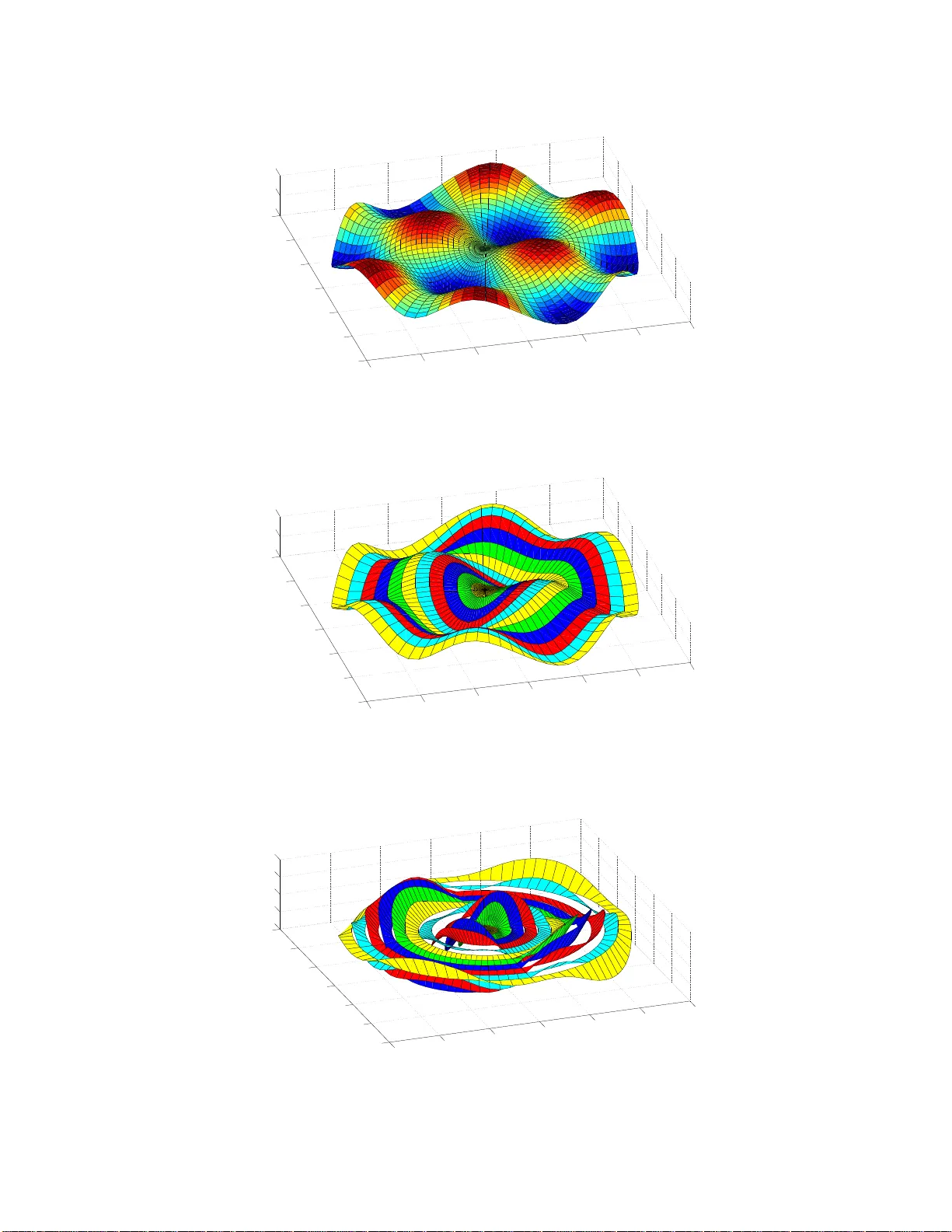
P atc h y Solutio n of a F rancis–Byrn es–Isid ori P artial Differen tial Equation 1 Cesar O. Aguilar 2 and Arth ur J. Krener 3 Abstract The solution to the nonlinear output regulation problem requir es one to solv e a first order PDE, kn o wn as t h e F rancis-Byrnes-Isidori (FBI) equat ions . In this pap er w e prop ose a metho d to compute approximate solutions to the FBI equ ations when the zero dynamics of the plant are hyp erb olic and the exosystem is t wo-dimensional. With our metho d we are able to pr o duce appr o ximations that con v erge un iformly to the tru e solution. Our method relies on the p erio d ic nature of tw o-dimensional analytic cen ter manifolds. 1 In tro ductio n Consider the control system ˙ x = f ( x, u, w ) ˙ w = s ( w ) y = h ( x, u, w ) (1) where x ∈ R n is the state v ariable, u ∈ R m is the con trol v ariable, w ∈ R q is an exogenous v ariable, and y ∈ R p is the o ut put v ariable. The maps f : R n × R m × R q → R n , s : R q → R q and h : R n × R m × R q → R p are all assumed to be sufficien tly smo o th and satisfy f (0 , 0 , 0) = 0, s (0) = 0, and h (0 , 0 , 0) = 0. The v ariable w represen ts a disturbance and/or a reference signal, and its dynamics are c ommonly referred to as the exosystem . The state fe e d b ack r e gulator pr oblem [8] is to find a state f eedbac k control u = α ( x, w ), with α (0 , 0) = 0, suc h that the equilibrium x = 0 of the dynamical system ˙ x = f ( x, α ( x, 0 ) , 0) is expo nen tially stable, and suc h that for eac h sufficien tly small initial condition ( x 0 , w 0 ) the solution of (1) with u = α ( x, w ) satisfies lim t →∞ y ( t ) = 0 . A c har a cterization of the state feedbac k regulato r problem for linear systems w as giv en b y F rancis [3] and later generalized to nonlinear sys tems b y Isidori and Byrnes [8]. As 1 Research supp orted in part by AFOSR and NSF. 2 National Research Co uncil Postdoctor al F ello w, Department of Applied Ma thematics, Nav al Postgra d- uate Schoo l, Mon ter ey , CA 939 4 3, coaguil a@nps .edu 3 Distinguished Visiting Pr ofessor, Department of Applied Ma thematics, Nav al Postgradua te Schoo l, Mon- terey , CA 93943, ajk rener@ nps.e du 1 sho wn in [8], the solv abilit y of the regulator problem can b e reduced to the solv a bilit y of a system of partial differen t ia l e quations (PDEs), whic h in the linear cas e reduce to the Sylv ester t yp e equation obtained b y F rancis . F or this reason, w e refer to these equations as the F rancis–Byrnes–Isidori (FBI) PDEs. F or completeness, w e state the main result of [8] (for the definition of P oission stabilit y used b elo w see R emark 1.1). Theorem 1.1 (Isidori–Byrnes ) . Assume that the e quili b ri um w = 0 o f the exosystem is Lyapunov stable and ther e is a neighb orho o d o f w = 0 in which every p oint is Poisson stable. Assume further that the p air  ∂ f ∂ x (0 , 0 , 0) , ∂ f ∂ u (0 , 0 , 0)  (2) is stabiliz a ble. Then the state fe e db ack r e gulator pr oblem is solvable if an d only if ther e exists C k ( k ≥ 2 ) m a ppings π : Ω → R n , with π (0) = 0 , and κ : Ω → R m , with κ (0) = 0 , b oth define d in a ne ighb orho o d Ω ⊆ R q of w = 0 , an d sa tisfying ∂ π ∂ w ( w ) s ( w ) = f ( π ( w ) , κ ( w ) , w ) 0 = h ( π ( w ) , κ ( w ) , w ) . (3) Giv en a solution pair ( π , κ ) to the FBI equations (3), a state feedbac k solving the regulator problem is giv en b y α ( x, w ) = κ ( w ) + K ( x − π ( w )) where K ∈ R m × R n is a ny feedbac k matrix r endering the pair (2) asymptotically stable. In general, solutions t o the FBI equations, b eing singular quasilinear PDEs with constrain ts, ma y no t exist. Ho w ever, for a class of con trol- affine systems , it is sho wn in [8] that the solv abilit y of the F BI equations is a prop ert y of the zero dynamics of (1). Roughly sp eaking, if the zero dynamics of (1) has a h yp erb olic equilibrium at the origin then a solution to the FBI equations exists b y the cen ter ma nif o ld theorem [2]. It is kno wn, how ev er, tha t cen ter manifolds suffer from a num b er of subtle prop erties asso ciated with uniqueness and differen tiability [12]. D espite these difficulties, a C ∞ dynamical system p ossess a C k cen ter manifold for eac h k ≥ 1, and moreo ve r, it is p ossible to obtain appro ximate solutions of arbitrarily high-o rder via T aylor series [2]. In this r esp ect, Huang and Rugh [6] a nd Krener [9] pro vide a metho d to compute approximate solutions to the FBI equations via T a ylor p olynomials, yie lding a ppro ximate output regulation. A shortcoming of this a pproac h is that the doma in on whic h the series approx ima t io n yields satisfactory results is not guarantee d to enlarge significan tly b y computing higher order approxim ations. T his can b e a serious dra wback as the num ber of monomials in q v ariables of degree d is  q + d − 1 d  , a n umber gro wing rapidly in d . Moreo v er, p olynomial appro ximations to ( π , κ ) can lead to destabilizing effects when the order of the approx imatio n increases. 2 In this pap er, we presen t a metho d to compute solutions to the FBI equations for the class of real analytic SISO con tro l-affine systems ˙ x = f ( x ) + g ( x ) u ˙ w = s ( w ) y = h ( x ) + p ( w ) (4) where f : R n → R n , g : R n → R n , s : R q → R q , h : R n → R , and p : R q → R are real analytic ab o ut t he origin. F urthermore, we will restrict o ur considerations to t wo- dimensional exosyste ms, i.e., q = 2, whose linear part con tains non- zero eigenv alues. Our metho d is based on the existence a nd uniquenes s results for tw o-dimensional analytic cen ter manifolds in [1] and on the high- order patch y metho d of Na v asca and Krener [10]. A ke y strength of our approxim a tion metho d, whic h r elies on the p erio dic nature of the solution to the F BI equations for (4), is the reduction of the computatio nal effort inheren t in a direct T a ylor p olynomial approximation. The organization of this pap er is a s fo llows. In Section 2 we briefly summarize the k ey insight provide d in [8 ] on ho w the solv abilit y o f the F BI equations can b e reduced to the problem o f solving a cen ter manifold equation pro vided the zero dynamics of (4) are h yp erb olic. With this simplification, w e sho w ho w the standard stability assumptions on the exosystem lead to a direct application o f the results in [1] to deduce uniquene ss of solutions to the FBI equations of (4). In Section 3, w e describ e our metho d to compute a high-order piecewis e smo oth approximation t o the solution of the FBI equations and pro v e that a sequence of approximations generated b y our metho d con v erges uniformly to the true solution. Finally , in Section 4 w e illustrate our metho d on examples and then mak e some concluding remarks. Remark 1.1. Henceforth, it will b e implicitly assumed that the exosystem has an equilib- rium w = 0 that is Lyapuno v stable and that there is a neigh b o r ho o d of w = 0 in whic h ev ery p oin t is P oisson stable. W e will refer to this t yp e of stability as neutr al stability . By P oisson stability w e mean the follo wing. An initial condition x 0 of the dynamical system ˙ x = f ( x ) is P oisson stable if the flow Φ f t ( x 0 ) of the v ector field f is defined for all t ∈ R and for eac h neigh b o urho o d U o f x 0 and for each real n umber T > 0, there exists a time t 1 > T suc h t ha t Φ f t 1 ( x 0 ) ∈ U and a time t 2 < − T suc h that Φ f t 2 ( x 0 ) ∈ U . 2 Real analyt i c and p erio dic solutio ns t o th e FBI equa- tions As sho wn in [8], a k ey simplification in the problem of solving t he FBI equations for a system of the form (4) consists in reducing it to the problem of solving a cente r manifold equation 3 for the zero dynamics of (4). F ollowing [8] a nd using the no w standard not a tion in [7], assume t hat the triplet { f , g , h } has relativ e degree 1 ≤ r < n at x = 0 and let ( z , ξ ) denote the standard normal co ordinates, where ξ = ( h ( x ) , L f h ( x ) , . . . , L r − 1 f h ( x )) and z is suc h that L g z = 0. In the ( z , ξ ) co ordinates, (4) tak es the form ˙ z = f 0 ( z , ξ ) ˙ ξ 1 = ξ 2 , . . . , ˙ ξ r − 1 = ξ r ˙ ξ r = b ( z , ξ ) + a ( z , ξ ) u ˙ w = s ( w ) y = ξ 1 + p ( w ) . (5) The zero dynamics o f (4) are giv en b y the dynamical system ˙ z = f 0 ( z , 0 ) . (6) Define functions ϕ i : R q → R by ϕ i ( w ) = − L i − 1 s p ( w ), 1 ≤ i ≤ r , set ϕ ( w ) = ( ϕ 1 ( w ) , . . . , ϕ r ( w )), and let u e ( x, w ) = − L r f h ( x ) + L r s p ( w ) L g L r − 1 f h ( x ) . Then it is straightforw ard to v erify tha t if φ satisfies the PDE ∂ φ ∂ w ( w ) s ( w ) = f 0 ( φ ( w ) , ϕ ( w )) (7) then π ( w ) := ( φ ( w ) , ϕ ( w )) and κ ( w ) := u e ( π ( w ) , w ) constitute a solution pair to the FBI equations of (5). If the origin of (6) is hy p erb olic, then ( 7) is the equation that is satisfied b y any cen ter manifold { ( z , w ) : z = φ ( w ) } of the dynamical system ˙ z = f 0 ( z , ϕ ( w )) ˙ w = s ( w ) . (8) Hence, in the h yp erb o lic case, the problem of solving the FBI equations asso ciated to the original system (4) is reduced to solving the cen ter manifold equation asso ciated to (8 ) . Although this simplification is significan t, solutions to cen ter manifo lds suffer from subtleties asso ciated with uniqueness and differen tia bilit y [12]. F or example, it is kno wn that an analytic dynamical sys tem do es not generally po sses an analytic cen ter manifold, thereb y forcing one to seek a center manifold solution that is only C k ( k = 2 , 3 , . . . ) and thus not necessarily unique. As an example, the p olynomial dynamical system ˙ z = − z + w 2 1 + w 2 2 ˙ w 1 = − w 2 − 1 2 w 1 ( w 2 1 + w 2 2 ) ˙ w 2 = w 1 − 1 2 w 2 ( w 2 1 + w 2 2 ) 4 whic h is of the form (8), has the prop erty that eac h cen ter manifold ha s T a ylor series ∞ X i =1 ( i − 1) !( w 2 1 + w 2 2 ) i whic h has v anishing radius of con vergenc e. D espite these difficulties , a sp ecial case for whic h sharp uniqueness and differentiabilit y results exist is for tw o-dimensional cen ter manifolds, and is give n b y the follow ing theorem due to Aulbach [1 ]. Theorem 2.1 (Aulbach) . Consider the or dinary differ ential e quation ˙ z = B z + Z ( w 1 , w 2 , z ) ˙ w 1 = − w 2 + P ( w 1 , w 2 , z ) ˙ w 2 = w 1 + Q ( w 1 , w 2 , z ) (9) wher e w 1 , w 2 ∈ R , z ∈ R n , and P , Q, and Z ar e r e al analytic functions ab out the origin and have T aylor se rie s b e ginning with quadr atic terms. Supp ose that the matrix B has no eigenvalues on the ima ginary axis. If the lo c al c enter manifol d dynamics of (9) a r e Lyapunov stable and non-attr active then (9) ha s a uniquely determine d lo c al c enter manifold which is analytic and gener ate d by a famil y of p erio dic solutions. Aulbac h’s result has a direct application to the output regulatio n problem, as giv en by the follow ing theorem. Theorem 2.2. Supp ose that in (4) the exosystem is two-dime n sional a n d ∂ s ∂ w (0) has n on- zer o eigenval ues. Supp ose that f , g , h and p ar e r e al analytic mappi n gs ab out x = 0 and w = 0 , r esp e ctively, an d that the triple { f , g , h } has a wel l-defin e d r elative de gr e e 1 ≤ r < n at x = 0 . If the zer o dynamics of (4) ar e hyp erb o l i c , then ther e exist unique and r e al analytic mappings ( π , κ ) solv ing the asso ciate d FBI e quations o f (4) . Pro of. By assumption and neutral stabilit y of the exosystem, the eigen v alues of the exosys- tem are non-zero and purely imaginary . Indeed, if the eigenv alues w ere not purely imaginary then w = 0 w ould nece ssarily b e either a rep elling or an att r activ e equilibrium, con tra dicting the assumption o f neutral stabilit y . No w since B := ∂ f 0 ∂ z (0 , 0) con tains eigen v alues off the imaginary axis, there exists an analytic co ordiante c hange [1 1 ] a b out t he origin suc h that (8) tak es the form ˙ z = B z + Z ( w 1 , w 2 , z ) ˙ w 1 = − w 2 + P ( w 1 , w 2 ) ˙ w 2 = w 1 + Q ( w 1 , w 2 ) , (10) where P , Q and Z are analytic at the origin and ha v e T a ylor series b eginning with quadratic terms. F rom (10), we can observ e that the dynamics of an y cente r manifold o f (10) are 5 equiv a len t t o the exosystem dynamics, whic h b y assumption are L yapuno v stable and non- attractiv e. Aulbac h’s theorem completes the pro of.  Remark 2.1. Theorem 2 .2 actually holds for more general MIMO con trol-affine system s with m = p . In [5], it is sho wn that if the comp osite con trol-affine system ˙ x = f ( x, w ) + m X i =1 g i ( x, w ) u i ˙ w = s ( w ) y = h ( x, w ) has a w ell- defined relativ e degree a t ( x, w ) = ( 0 , 0), then the asso ciated FBI equations are solv able if the zero dynamics of the comp osite system are h yp erb olic. In t his case, the FBI equations reduce to a cen ter manif o ld equation of the for m (7 ) so that Aulbach’s theorem can b e applied when the exosystem is tw o-dimensional. Example 2.1. The dynamics of a cart and inv erted p endulum system can be written in the form ˙ x 1 = x 2 ˙ x 2 = u ˙ x 3 = x 4 ˙ x 4 = g ℓ sin( x 3 ) − 1 ℓ cos( x 3 ) u (11) where x 1 is the p osition of the cart, x 3 is the a ng le the p endulum make s with the v ertical, g is the a cceleration due to gr a vity , ℓ is the length of the ro d, and u is the control force. With h ( x ) = x 1 , t he system has relativ e degree r = 2 at x = 0 , and therefore ( ξ 1 , ξ 2 ) = ξ ( x ) = ( h ( x ) , L f h ( x )) = ( x 1 , x 2 ). With ( z 1 , z 2 ) = z ( x ) = ( x 3 , x 4 + x 2 ℓ cos( x 3 )), the zero dynamics are giv en b y ˙ z 1 = z 2 ˙ z 2 = g ℓ sin( z 1 ) , whose linearization has eigenv alues ± p g ℓ . Hence, with system out put y = x 1 + p ( w ) ( p real analytic) and a t w o- dimensional real analytic exosyste m whose linearization has non-zero eigen v alues, there exists a unique and real a nalytic solution to the asso ciated FBI equations of the cart a nd inv erted p endulum system (11).  3 Computation of the center manifold In this section w e outline a metho d to compute the solution to the FBI equations in the case of t w o- dimensional exosystem and real analytic data . As describ ed in the previous section, 6 for the nonlinear control systems in consideration, the solv abilit y of t he FBI equations can b e reduced to solving a cen ter manifold equation f or a dynamical system of the form ˙ z = B z + ¯ Z ( w 1 , w 2 , z ) ˙ w 1 = − w 2 + P ( w 1 , w 2 ) ˙ w 2 = w 1 + Q ( w 1 , w 2 ) , (12) where w = ( w 1 , w 2 ) ∈ R 2 , z ∈ R n , ¯ Z , P , and Q are real analytic mappings, a nd the eigen v alues of B ha ve non-zero real parts. W e will therefore limit our considerations to solving the cen ter manifold equation for (12). It will b e assumed that the w -dynamics hav e w = 0 as a Ly a punov stable and non-a t t ractiv e equilibrium. By Theorem 2.1, t here exists a unique analytic mapping φ ( w 1 , w 2 ), defined lo cally ab out w = 0, solving the cen ter manifold PDE asso ciated to (1 2 ). Our metho d is b est describ ed on the represen tation of (12) in p olar co ordinates. Hence, w e apply the tranfor mation ( w 1 , w 2 , z ) = ( r cos θ , r sin θ , z ) to (1 2) yielding a system o f the form ˙ r = r ˆ R ( θ , r ) ˙ θ = 1 + ˆ Θ( θ , r ) ˙ z = B z + ˆ Z ( θ , r , z ) (13) where ˆ R, ˆ Θ , ˆ Z are analytic functions con v erging for each θ ∈ [0 , 2 π ] a nd | r | ≤ a , k z k ≤ a , where a > 0 is a p ositiv e constan t . D efine ˆ f ( θ , r , z ) = B z + ˆ Z ( θ , r, z ). The cen ter manifold PDE for (13) is ˆ f ( θ , r, ψ ( θ , r )) = ∂ ψ ∂ θ [1 + ˆ Θ( θ , r )] + ∂ ψ ∂ r r ˆ R ( θ , r ) (14) for the unknown analytic mapping ψ ( θ , r ) (= φ ( r cos θ , r sin θ )). The mapping ψ has a p ow er series represen tation ψ ( θ , r ) = ∞ X i =1 e i ( θ ) r i con v erging in a cylinder of the form θ ∈ [0 , 2 π ], | r | ≤ ǫ , and with 2 π -p erio dic co efficien ts e i ( θ ) [1]. By eliminating the time v ariable t , (13) can b e reduced t o dr dθ = r R ( θ , r ) (15a) dz dθ = B z + Z ( θ , r, z ) . (15b) Define f ( θ , r , z ) = B z + Z ( θ , r, z ). F ro m (14) it follows that f ( θ , r, ψ ( θ , r )) = ∂ ψ ∂ θ + ∂ ψ ∂ r dr dθ . (16) 7 W e now giv e a brief sk etc h of o ur metho d. Let r ( θ ) b e a solution to (15a) and define the mapping Ψ( θ , σ ) = ψ ( θ , r ( θ ) + σ ) for θ ∈ [0 , 2 π ] and | σ | small. W e note that, with r = r ( θ ) substituted into the RHS of (15b), the curv e Ψ( θ , 0) = ψ ( θ , r ( θ )) is the solution to (15b) with initial condition z (0) = ψ (0 , r (0)). F or | σ | sufficien tly small, w e ha v e a p ow er series represen tation Ψ( θ , σ ) = Ψ( θ, 0) + ∞ X i =1 ∂ i Ψ ∂ σ i ( θ , 0) σ i i ! (17) con v erging for all θ ∈ [0 , 2 π ] and ha ving 2 π -p erio dic co efficien ts ∂ i Ψ ∂ σ i ( θ , 0). In fa ct, it is easy to see that ∂ i Ψ ∂ σ i ( θ , 0) = ∂ i ψ ∂ r i ( θ , r ( θ )) . (18) By construction, the mapping Ψ is a p erturbation of ψ ( θ , r ( θ )) in the radial direction, the amoun t of p erturbat ion g iv en by the parameter σ . Our metho d is based on computing the T a ylor series appro ximation Ψ N ( θ , σ ) = Ψ( θ , 0) + N X i =1 ∂ i Ψ ∂ σ i ( θ , 0) σ i i ! and using it to build t he cen ter manifold along r ( θ ) in t he radial direction. Ha ving follow ed Ψ N along a small annular regio n, sa y of the form { ( θ , r ) : 0 ≤ θ ≤ 2 π , r ( θ ) ≤ r < r ( θ ) + ǫ } , w e compute a new radial curv e θ 7→ ˜ r ( θ ) with initial condition ˜ r (0 ) = r (0) + ǫ , compute the new corresp onding T a ylor series appro ximation ˜ Ψ N , and then con tinue building the cente r manifold by following ˜ Ψ N along the annular regio n { ( θ , r ) : 0 ≤ θ ≤ 2 π , ˜ r ( θ ) ≤ r < ˜ r ( θ ) + ˜ ǫ } . This pro cess is rep eated and the a nnular regions, along with the corresp onding appro xima- tions, a re patch ed tog ether to form a piecewise smo oth approximation to the true solution ψ . Remark 3.1. T o compute the T a ylor series a ppro ximations Ψ N it is necess ar y to compute the θ -dep enden t co efficien ts appearing in (17), whic h can b e done in the following wa y . F rom the definition o f Ψ, a direct computations giv es ∂ Ψ ∂ θ = ∂ ψ ∂ θ ( θ , r ( θ ) + σ ) + ∂ ψ ∂ r ( θ , r ( θ ) + σ ) dr dθ 8 whic h when com bined with (16) yields ∂ Ψ ∂ θ = f ( θ , r ( θ ) + σ, Ψ ( θ , σ )) . (19) Using (19), w e can no w write a do wn linear inhomogeneous OD E for the co efficien t ∂ i Ψ ∂ σ i ( θ , 0). Indeed, differen tia t ing (19) with r esp ect to σ , and in terc hanging the o rder of differen tiat ion, yields ∂ ∂ θ  ∂ Ψ ∂ σ ( θ , σ )  = ∂ f ∂ z ( θ , r ( θ ) + σ, Ψ( θ , σ )) ∂ Ψ ∂ σ ( θ , σ ) + ∂ f ∂ r ( θ , r ( θ ) + σ, Ψ( θ , σ )) and therefore ∂ ∂ θ  ∂ Ψ ∂ σ ( θ , 0)  = A ( θ ) ∂ Ψ ∂ σ ( θ , 0) + ∂ f ∂ r ( θ , r ( θ ) , Ψ( θ , 0)) where the matrix A ( θ ) = ∂ f ∂ z ( θ , r ( θ ) , Ψ( θ , 0)). In general, it can b e v erified b y induction that ∂ ∂ θ  ∂ i Ψ ∂ σ i ( θ , 0)  = A ( θ ) ∂ i Ψ ∂ σ i ( θ , 0) + F i  θ , Ψ( θ , 0) , ∂ Ψ ∂ σ ( θ , 0) , . . . , ∂ i − 1 Ψ ∂ σ i − 1 ( θ , 0)  (20) for some mappings F i , i ≥ 2. With the previous constructions in mind, w e are no w ready to describ e an algorithm for computing the solution ψ to t he cen ter manifo ld equation (16) . 1. Let N ≥ 1 b e a fixed p ositive integer and let ψ N 0 ( θ , r ) = N X i =1 e i ( θ ) r i , that is, ψ N 0 is simply the N t h order T a ylor a ppro ximation of ψ in r . T o compute ψ N 0 , one can use the method in [6] to generate a N th order T a ylor p olynomial appro ximation of φ ( w 1 , w 2 ), sa y φ N ( w 1 , w 2 ), and then simply ψ N 0 ( θ , r ) = φ N ( r cos θ , r sin θ ). Set Ψ 0 = ψ and set r − 1 ( θ ) = 0 f or θ ∈ R . The initial approximation ψ N 0 will b e accepted in a n ann ular region of the fo r m { ( θ , r ) : 0 ≤ θ ≤ 2 π , 0 ≤ r < r 0 ( θ ) } where r 0 ( θ ) is the solution to (15 a) with some prescrib ed initial condition r 0 (0) = ǫ 0 > 0. T o compute accurate n umerical solutions to r 0 , we solv e a BVP using (15a) with b oundary conditions r (0) = r (2 π ) = ǫ 0 and constan t initial guess ǫ 0 on [0 , 2 π ]. 2. Define Ψ 1 ( θ , σ ) = ψ ( θ , r 0 ( θ ) + σ ). F rom (17 ), Ψ 1 can b e appro ximated by the truncated series Ψ N 1 ( θ , σ ) = Ψ 1 ( θ , 0) + N X i =1 ∂ i Ψ 1 ∂ σ i ( θ , 0) σ i i ! 9 for | σ | small. T o obtain accurate nume rical solutions to the co efficien ts ∂ i Ψ 1 ∂ σ i ( θ , 0), w e solv e BVPs using the OD Es (2 0) with b oundary conditions ∂ i Ψ 1 ∂ σ i (0 , 0) = ∂ i Ψ 1 ∂ σ i (2 π , 0) and initial guesses ∂ i Ψ 1 ∂ σ i ( θ , 0) ≈ ∂ i ψ N 0 ∂ r i ( θ , r 0 ( θ )) . Similarly , to compute Ψ 1 ( θ , 0) = ψ ( θ , r 0 ( θ )) w e solv e a BVP using (15b) with b oundary conditions z (0 ) = z ( 2 π ) and initial guess Ψ 1 ( θ , 0) ≈ ψ N 0 ( θ , r 0 ( θ )) . Ha ving computed Ψ 1 ( θ , 0) , ∂ Ψ 1 ∂ σ ( θ , 0) , . . . , ∂ N Ψ 1 ∂ σ N ( θ , 0), w e obtain an approximation ψ 1 ( θ , r ) to ψ ( θ , r ) defined by ψ 1 ( θ , r ) = Ψ N 1 ( θ , r − r 0 ( θ )) whic h is accepted in the region { ( θ , r ) : 0 ≤ θ ≤ 2 π , r 0 ( θ ) ≤ r < r 0 ( θ ) + ǫ 1 } (21) for some desired ǫ 1 > 0 . In this w ay , w e ha ve extended our original approximation ψ 0 of ψ to the domain (21). Our running appro ximatio n of ψ is giv en b y ψ ( θ , r ) ≈    ψ 0 ( θ , r ) , 0 ≤ r < r 0 ( θ ) , ψ 1 ( θ , r ) , r 0 ( θ ) ≤ r ≤ r 0 ( θ ) + ǫ 1 for θ ∈ [0 , 2 π ]. 3. W e no w pro ceed to augment to our running approx imat io n a mapping ψ 2 , that will b e defined o n an an ann ular region surrounding the domain of ψ 1 , in the following w ay . W e first compute the solution r 1 ( θ ) to (15a) with initial condition r 1 (0) = r 0 (0) + ǫ 1 . As in Step 2, t his is done b y solving a BVP using (15a) with b oundary conditions r (0) = r (2 π ) = r 0 (0) + ǫ 1 and taking t he curv e r 0 ( · ) + ǫ 1 as an initial guess to r 1 . Here w e note that, to a void o ve rla pping doma ins of definition b et ween ψ 1 and ψ 2 , the domain (21) of ψ 1 is redefined to b e { ( θ , r ) : 0 ≤ θ ≤ 2 π , r 0 ( θ ) ≤ r < r 1 ( θ ) } . 4. W e now rep eat Step 3 with r 1 ( θ ) a nd build a n approx ima t io n to Ψ 2 ( θ , σ ) = ψ ( θ , r 1 ( θ ) + σ ) of the form Ψ N 2 ( θ , σ ) = Ψ 2 ( θ , 0) + N X i =1 ∂ i Ψ 2 ∂ σ i ( θ , 0) σ i i ! , 10 for 0 ≤ σ ≤ ǫ 2 and ǫ 2 > 0 sufficien tly small. The co efficien ts ∂ i Ψ 2 ∂ σ i ( θ , 0) are computed b y solving BVPs using the ODEs (20) with b oundary conditions ∂ i Ψ 2 ∂ σ i (0 , 0) = ∂ i Ψ 2 ∂ σ i (2 π , 0) and initial guesses ∂ i Ψ 2 ∂ σ i ( θ , 0) ≈ ∂ i Ψ 1 ∂ σ i ( θ , 0) . That is, we use t he previously computed co efficien ts as initial guesses f or the curren t co efficien ts. Similarly , to compute Ψ 2 ( θ , 0) = ψ ( θ , r 1 ( θ )) we solv e a BVP using (15b) with b oundary conditions z (0) = z (2 π ) and initia l guess Ψ 2 ( θ , 0) ≈ ψ 1 ( θ , r 1 ( θ )) . Ha ving computed Ψ 2 ( θ , 0) , ∂ Ψ 2 ∂ σ ( θ , 0) , . . . , ∂ N Ψ 2 ∂ σ N ( θ , 0), w e obtain the approximation ψ 2 ( θ , r ) = Ψ N 2 ( θ , r − r 1 ( θ )) whic h is accepted in the region { ( θ , r ) : 0 ≤ θ ≤ 2 π , r 1 ( θ ) ≤ r < r 1 ( θ ) + ǫ 2 } . (22) In this w ay , we extend o ur appro ximation o f ψ ( θ , r ) to the a nnulus (2 2) and our running appro ximation is ψ ( θ , r ) ≈            ψ 0 ( θ , r ) , 0 ≤ r < r 0 ( θ ) , ψ 1 ( θ , r ) , r 0 ( θ ) ≤ r < r 1 ( θ ) , ψ 2 ( θ , r ) , r 1 ( θ ) ≤ r ≤ r 1 ( θ ) + ǫ 2 for θ ∈ [0 , 2 π ]. 5. Steps 4-5 can no w b e iterated. Indeed, supp ose w e ha ve computed an approx imatio n ψ k ( θ , r ) to ψ ( θ , r ) o f t he form ψ k ( θ , r ) = Ψ N k ( θ , r − r k − 1 ( θ )), and defined in the region { ( θ , r ) : 0 ≤ θ ≤ 2 π , r k − 1 ( θ ) ≤ r < r k − 1 ( θ ) + ǫ k } , (23) where Ψ k ( θ , σ ) = ψ ( θ , r k − 1 ( θ ) + σ ), Ψ N k ( θ , σ ) = Ψ k ( θ , 0) + N X i =1 ∂ i Ψ k ∂ σ i ( θ , 0) σ i i ! and r k − 1 ( θ ) is the solution to (1 5 a) with initial condition r k − 1 (0) = Σ k − 1 i =0 ǫ i . T o extend our curren t approximation of ψ b ey ond the domain of ψ k , w e b egin b y computing the solution r k ( θ ) to (15 a) with initia l condition r k (0) = r k − 1 (0) + ǫ k . This is do ne by 11 solving a BVP using (15a) with b oundary conditio ns r (0) = r (2 π ) = r k − 1 (0) + ǫ k and initial guess r k − 1 ( · ) + ǫ k . Let now Ψ k +1 ( θ , σ ) = ψ ( θ , r k ( θ ) + σ ) and f orm Ψ N k +1 ( θ , σ ) = Ψ k +1 ( θ , 0) + N X i =1 ∂ i Ψ k +1 ∂ σ i ( θ , 0) σ i i ! . The co efficien ts ∂ i Ψ k +1 ∂ σ i ( θ , 0) are computed b y solving BVPs using the ODEs ( 2 0) with b oundary conditions ∂ i Ψ k +1 ∂ σ i (0 , 0) = ∂ i Ψ k +1 ∂ σ i (2 π , 0) and initial guesses ∂ i Ψ k +1 ∂ σ i ( θ , 0) ≈ ∂ i Ψ k ∂ σ i ( θ , 0) . Similarly , to compute Ψ k +1 ( θ , 0) w e solv e a BVP using (15b) with b oundary conditions z (0) = z (2 π ) and initial guess Ψ k +1 ( θ , 0) ≈ ψ k ( θ , r k ( θ )) . Ha ving computed Ψ k +1 ( θ , 0) , ∂ Ψ k +1 ∂ σ ( θ , 0) , . . . , ∂ N Ψ k +1 ∂ σ N ( θ , 0), we o btain the appro ximation ψ k +1 ( θ , r ) = Ψ N k +1 ( θ , r − r k ( θ )) whic h is accepted in the region { ( θ , r ) : 0 ≤ θ ≤ 2 π , r k ( θ ) ≤ r < r k ( θ ) + ǫ k +1 } . (24) T o av oid o ve rla pping the domains of ψ k and ψ k +1 , the domain of definition (23) o f ψ k is redefined to b e { ( θ , r ) : 0 ≤ θ ≤ 2 π , r k − 1 ( θ ) ≤ r ≤ r k ( θ ) } . 6. After iterating Steps 4-5 a k ≥ 1 n um b er of times, w e obta in the following piecewise smo oth approximation to ψ ( θ , r ): ψ ( θ , r ) ≈ ˜ ψ k ( θ , r ) :=                  ψ 0 ( θ , r ) , 0 ≤ r < r 0 ( θ ) , ψ 1 ( θ , r ) , r 0 ≤ r < r 1 ( θ ) , . . . . . . ψ k ( θ , r ) , r k − 1 ≤ r ≤ r k ( θ ) (25) for θ ∈ [0 , 2 π ]. Let us mak e a few remarks a b out our a lg orithm. Remark 3.2. 1. The co efficien ts ∂ i Ψ ∂ σ i ( θ , 0), i = 0 , 1 , . . . , are computed b y solving BVP problems f or mainly tw o reasons: (1) they are known a priori to b e p erio dic, and (2) w e hav e go o d appro ximations of them from the previously computed co efficien ts. 12 2. The main computational effort of o ur metho d is in computing the co efficien ts ∂ i Ψ ∂ σ i ( θ , 0). F rom ( 2 0), w e see tha t the O D E for ∂ i Ψ ∂ σ i ( θ , 0) is linear in ∂ i Ψ ∂ σ i ( θ , 0) and is p olynomial in the previously computed Ψ( θ , 0) , . . . , ∂ i − 1 Ψ ∂ σ i − 1 ( θ , 0). Henc e, a w ay to sp eed up the computation is to solv e for the co efficien ts ∂ i Ψ ∂ σ i ( θ , 0) order-b y-or der. This can result in computational sa vings when the RHS of (20 ) is complicated to ev aluate or when n × N is large. 3. When the w -dynamics ar e g iv en by the harmonic oscillator ˙ w 1 = − w 2 ˙ w 2 = w 1 the computatio n of the radial curv es r ( θ ) is trivial and are giv en by the constan t curv es r ( θ ) = r (0). In this case, there is no need to redefine the outer b oundary of the success ive approximations ψ i when going from one ann ulus t o the other. 4. In order fo r t he algorithm to pro duce a meaningful approximation to ψ , the domain on whic h the approximation (25) is defined, namely { ( θ , r ) : 0 ≤ θ ≤ 2 π , 0 ≤ r ≤ r k ( θ ) } , m ust of course b e contained in the cylinder θ ∈ [0 , 2 π ], | r | ≤ ǫ on whic h ψ is defined. Since ǫ is not known a priori , the algor it hm m ust pro ceed from r k − 1 to r k b y ta king small incremen ts r k (0) − r k − 1 (0) = ǫ k and c ho osing r 0 (0) sufficien tly small. T o end this section, w e pro v e that t he sequence of approximations { ˜ ψ k } ∞ k =1 obtained from (25) con vergenc e uniformly to ψ . Theorem 3.1. Supp ose that ψ is define d on the cylin d e r Ω = { ( θ , r ) : 0 ≤ θ ≤ 2 π , 0 ≤ r ≤ ǫ } and let ˜ ǫ < ǫ b e chosen s o that i f r : [0 , 2 π ] → R is a tr aje ctory of (15a) with r ( 0 ) ≤ ˜ ǫ then r ( θ ) < ǫ . L et ˜ ψ k b e defi ne d as in (25) , wi th step- size r j (0) − r j − 1 (0) = ǫ j := 1 k +1 ˜ ǫ , for j = 0 , 1 , . . . , k . Then ˜ ψ k → ψ uniformly in ˜ Ω = { ( θ , r ) : 0 ≤ θ ≤ 2 π , 0 ≤ r ≤ r k ( θ ) } . Pro of. W e first note tha t the existence of ˜ ǫ follows b y Lyapuno v stabilit y of the exosystem. By construction, r j (0) = j +1 k +1 ˜ ǫ for j = 0 , 1 , . . . , k , and in particular r k (0) = ˜ ǫ , thereb y rendering the do ma in ˜ Ω indep enden t of k . Also w e note that, b y shrinking ˜ ǫ if necessary , b y Gron wall’s lemma it follow s that | ˜ r ( θ ) − ¯ r ( θ ) | ≤ | ˜ r (0) − ¯ r (0 ) | e K θ , (26) for all tra jectories θ 7→ ˜ r ( θ ) and θ 7→ ¯ r ( θ ) of (15a) suc h that 0 ≤ ˜ r ( 0) , ¯ r (0) ≤ ˜ ǫ , where K is a Lipsc hitz constan t independen t of θ . No w by definition, we hav e that Ψ j ( θ , σ ) = ψ ( θ , r j − 1 ( θ ) + σ ) a nd therefore ∂ N +1 Ψ j ∂ σ N +1 ( θ , σ ) = ∂ N +1 ψ ∂ r N +1 ( θ , r j − 1 ( θ ) + σ ) . 13 Hence, b y T aylor’s theorem, Ψ j ( θ , σ ) = Ψ N j ( θ , σ ) + 1 N ! Z σ 0 ( σ − τ ) N ∂ N +1 Ψ j ∂ σ N +1 ( θ , τ ) d τ = Ψ N j ( θ , σ ) + 1 N ! Z σ 0 ( σ − τ ) N ∂ N +1 ψ ∂ r N +1 ( θ , r j − 1 ( θ ) + τ ) dτ . Let C = max ( θ, r ) ∈ Ω k ∂ N +1 ψ ∂ r N +1 ( θ , r ) k , a nd w e note that C exists b y contin uit y of ∂ N +1 ψ ∂ r N +1 on the compact set Ω. W e t herefore hav e that k Ψ j ( θ , σ ) − Ψ N j ( θ , σ ) k ≤ C σ N +1 ( N + 1)! pro vided 0 ≤ σ ≤ r j ( θ ) − r j − 1 ( θ ) for θ ∈ [0 , 2 π ], fo r a ll j = 0 , 1 , . . . , k . No w since r j (0) ≤ ˜ ǫ for j = 0 , 1 , . . . , k , it follows b y (26) that | r j ( θ ) − r j − 1 ( θ ) | ≤ | r j (0) − r j − 1 (0) | e K θ ≤ 1 k +1 ˜ ǫ e 2 π K . Therefore, given ( θ , r ) ∈ ˜ Ω, sa y t hat r j − 1 ( θ ) ≤ r < r j ( θ ) fo r some j ∈ { 0 , 1 , . . . , k } , it follo ws tha t k ψ ( θ , r ) − ˜ ψ k ( θ , r ) k = k Ψ j ( θ , r − r j − 1 ( θ )) − ψ j ( θ , r − r j − 1 ( θ )) k = k Ψ j ( θ , r − r j − 1 ( θ )) − Ψ N j ( θ , r − r j − 1 ( θ )) k ≤ C ( N + 1)! ( r − r j − 1 ( θ )) N +1 ≤ C ( N + 1)!  1 k +1 ˜ ǫe 2 π K  N +1 . Hence, k ψ ( θ , r ) − ˜ ψ k ( θ , r ) k → 0 as k → ∞ uniformly in ˜ Ω. This completes t he pro of.  4 Examples In this section we presen t examples illustrat ing our metho d. Example 4.1. In this example w e ta k e a linear dynamical system of the form (12), whose cen ter manifold is easily computed, p erfor m a no nlinear c hange of co or dinates and arriv e at a nonlinear system on whic h we apply our metho d. The true solutio n f or the nonlinear system is then readily a v ailable and w e can compare the appro ximations pro duced b y our 14 metho d with the true soluiton. Consider then the linear dynamical system ˙ x 1 = x 2 + 1 2 w 1 + 1 2 w 2 ˙ x 2 = x 3 + 1 3 w 1 + 2 3 w 2 ˙ x 3 = − x 1 − 1 2 w 1 + 1 2 w 2 ˙ w 1 = − w 2 ˙ w 2 = w 1 . The cen ter manifold equation for this system in the unknow n mapping x = φ ( w ) is ∂ φ ∂ w ( w ) S w = C φ ( w ) + D w where x = ( x 1 , x 2 , x 3 ) , w = ( w 1 , w 2 ), and S =  0 − 1 1 0  , C =   0 1 0 0 0 1 − 1 0 0   , D =      1 2 1 2 1 3 2 3 − 1 2 1 2      . It is straightforw ard to v erify tha t φ ( w ) = ( − 1 3 w 1 , − 1 2 w 1 − 1 6 w 2 , − 1 2 w 1 − 1 6 w 2 ) is the unique solution to the cen ter manifold equation for t his system. Consider the co ordinate c ha ng e z = Z ( x ) = ( − 3 x 1 , 9 x 1 − 6 x 2 , − x 2 + x 3 + ρ ( − 3 x 1 , 9 x 1 − 6 x 2 )), where ρ : R 2 → R is a smo o th function. The sys t em in ( z , w ) co ordinates tak es the form of (12) with matrix B ha ving eigen v alues − 1 , 1 2 ± √ 3 i . By direct substitution, the solution to the cente r manifold equation of the sys t em in ( z , w ) co o rdinates is z = Z ( φ ( w )) = ( w 1 , w 2 , ρ ( w 1 , w 2 )), i.e., it is the graph o f the function ρ . F or purp oses of illustration we tak e the egg carton shap ed function ρ ( w 1 , w 2 ) = sin( w 1 ) sin( w 2 ), whose graph is show n in Figure 1. The patc hy approximation ˜ ψ k ( w 1 , w 2 ) = ( w 1 , w 2 , ˜ ρ ( w 1 , w 2 )) computed with our metho d with k = 10 a nn ular regions o f thic kness ǫ = 0 . 5 and o f order N = 2 is sho wn in Figure 2. Th e error b et w een the patch y appro ximation and the true solution is sho wn in Figure 3. Lastly , Figure 4 sho ws that in order to get a similar error b ound as with the patc hy approximation, one needs to use a p olynomial approximation of degree 19. Example 4.2. This example illustrates the loss of stability when using p olynomial ap- pro ximations. W e pro ceed as in Example 4 .1 but instead use the v o lcano t yp e function ρ ( x, y ) = sin( x 2 + y 2 ) e 1 − x 2 − y 2 , whose graph is sho wn in Figure 5. The patc h y appro ximatio n is show n in Figure 6 and the error in using the patch y approximation is sho wn in Figure 7. The patch y approximation is constructed with k = 60 annular regions of thic kness ǫ = 0 . 05 and of order N = 1, i.e., w e o nly use a first order T aylor series in the radial direction. F or 15 −6 −4 −2 0 2 4 6 −6 −4 −2 0 2 4 6 −1 0 1 w 1 w 2 Figure 1: T rue solutio n ρ ( w 1 , w 2 ) = sin( w 1 ) sin( w 2 ). −6 −4 −2 0 2 4 6 −6 −4 −2 0 2 4 6 −1 0 1 w 1 w 2 Figure 2: Patc h y solutio n ˜ ρ ( w 1 , w 2 ) with N = 2 and k = 10 . −6 −4 −2 0 2 4 6 −6 −4 −2 0 2 4 6 −0.04 −0.02 0 0.02 0.04 w 1 w 2 Figure 3: Error ρ ( w 1 , w 2 ) − ˜ ρ ( w 1 , w 2 ) with patch y solution with N = 2 and k = 10. 16 −6 −4 −2 0 2 4 6 −6 −4 −2 0 2 4 6 −0.02 −0.01 0 0.01 0.02 w 1 w 2 Figure 4: Error ρ ( w 1 , w 2 ) − ˜ ρ ( w 1 , w 2 ) with p o lynomial approx imat io n of degree 19. this example, p olynomial appro ximations of orders up to 30 where tested and it w as v erified that as one increases the order o f the p olynomial appro ximation the error in fact increases on the domain in consideration. −4 −3 −2 −1 0 1 2 3 4 −4 −2 0 2 4 −0.2 0 0.2 0.4 0.6 0.8 1 1.2 w 1 w 2 Figure 5: T rue solutio n ρ ( x, y ) = sin( x 2 + y 2 ) e 1 − x 2 − y 2 . Example 4.3. Consider the inv erted pendulum cart system from Example 2.1 with tw o- dimensional exosystem given b y ˙ w = s ( w ) =  w 2 − w 1 − aw 3 1  (27) where a > 0. System (27) is a sp ecial case of the unfor ced Duffing’s oscillator with no damping [4]. The equilibrium w = 0 of (27) is a cen ter and represen tativ e p erio dic solutions encircling w = 0 are sho wn in Figure 8. 17 −4 −3 −2 −1 0 1 2 3 4 −4 −2 0 2 4 −0.2 0 0.2 0.4 0.6 0.8 1 1.2 w 1 w 2 Figure 6: Patc h y solutio n ˜ ρ ( w 1 , w 2 ) with N = 1 and k = 60 . −4 −3 −2 −1 0 1 2 3 4 −4 −2 0 2 4 −8 −6 −4 −2 0 2 4 6 8 x 10 −3 w 1 w 2 Figure 7: Error ρ ( w 1 , w 2 ) − ˜ ρ ( w 1 , w 2 ) with patch y solution with N = 1 and k = 60. −2.5 −2 −1.5 −1 −0.5 0 0.5 1 1.5 2 2.5 −2.5 −2 −1.5 −1 −0.5 0 0.5 1 1.5 2 2.5 w 1 w 2 Figure 8: Unforced D uffing’s oscillator with no damping and a = 1 4 . 18 Let p ( w ) = − w 1 . As in Example 2.1, let ( z , ξ ) denote the standard normal co ordinat es, where z = ( x 3 , x 4 + x 2 ℓ cos( x 3 )) and ξ = ( h ( x ) , L f h ( x )) = ( x 1 , x 2 ). F ollowing the notatio n at the b eginning of § 2, let ϕ 1 ( w ) = − p ( w ) = w 1 and ϕ 2 ( w ) = − L s p ( w ) = w 2 . Then the differen tial equation (8) b ecomes ˙ z 1 = z 2 − 1 ℓ w 2 cos( z 1 ) ˙ z 2 = g ℓ sin( z 1 ) − 1 ℓ z 2 w 2 sin( z 1 ) − 1 ℓ 2 w 2 2 sin( z 1 ) cos( z 1 ) ˙ w 1 = w 2 ˙ w 2 = − w 1 − aw 3 1 (28) A pa t ch y approxim a tion to the solution φ ( w 1 , w 2 ) = ( φ 1 ( w 1 , w 2 ) , φ 2 ( w 1 , w 2 )) of the cen ter manifold equation of ( 28) was computed and is illustrat ed in Figures 9-10. The data g = 10, ℓ = 1 3 , and a = 1 4 w as used. The solution was computed with k = 40 and radial step at the initial angle θ = 0 w as tak en to b e ǫ i = 0 . 05, i = 1 , 2 , . . . , 25, and the order of the radial T a ylor p olynomials we r e c hosen as N = 2. −3 −2 −1 0 1 2 3 −3 −2 −1 0 1 2 3 −1.5 −1 −0.5 0 0.5 1 1.5 w 2 w 1 Figure 9: Patc h y appro ximatio n to φ 1 ( w 1 , w 2 ). The computed patc hy approximation t o the cen ter manifo ld PDE for (28) is used in an output track ing con troller of the form α ( z , w ) = κ ( w ) + K (( z , ξ ) − π ( w )) where π ( w ) = ( φ ( w ) , ϕ ( w )) and κ ( w ) = u e ( π ( w ) , w ), where the gain matrix K is chose n as the solution to an LQR problem for the linearization of the in verted p endulum. In the LQR problem, the matrices Q = diag ( 4 , 4 , 4 , 4) and R = 1 we re c hosen. A sim ulation is p erformed in whic h the p endulum is initialized at an angle of 15 degrees from the v ertical and the cart is initialized at − 0 . 25 from the origin. The reference tra jectory , y ref ( t ) = w 1 ( t ), is c hosen with initial condition y ref (0) = 1 . 2. The results of the sim ulation are sho wn in Figures 11-12. 19 −3 −2 −1 0 1 2 3 −3 −2 −1 0 1 2 3 −5 0 5 w 2 w 1 Figure 10: Patc h y appro ximation to φ 2 ( w 1 , w 2 ). 0 5 10 15 20 25 30 35 40 −2 −1.5 −1 −0.5 0 0.5 1 1.5 time [sec] y ref (t) y(t) Figure 11: Output y ( t ) = x 1 ( t ) and reference y ref ( t ) = w 1 ( t ). 0 5 10 15 20 25 30 35 40 −0.5 0 0.5 1 1.5 time [sec] Figure 12: T ra cking error e ( t ) = y ( t ) − y ref ( t ). 20 5 Conclus ion W e hav e presen ted a metho d to compute solutions to the FBI equations of real ana lytic con trol- a ffine systems with t w o - dimensional exosystems. Our tec hnique is based on the patc hy metho d in [10] and on the results in [1] for uniqueness of solutions of tw o-dimensional real analytic cen ter manifolds. In comparison with direct T a ylor p olynomial approximations [6, 9], our metho d lessens the computational effort needed to pro duce appro ximate solutions b y taking in t o account the p erio dic nature of a tw o-dimensional exosystem. W e prov ed that our metho d generates a sequence of approximations conv erging unifor mly to the true solution. References [1] B. Aulbac h, A c lassic al appr o ac h to the analyticity pr oblem of c enter mani f o lds , Journal of Applied Mathematics and Ph ysics, V ol. 36, No. 1, pp.1-2 3, 1985. [2] J. Carr, Applic ations of C entr e Manifolds The ory , Springer-V erlag, 1981. [3] B.A. F rancis, The li n e ar multivariable r e gulator pr oblem , SIAM J. Con trol Optim., 15, pp. 486-5 05, 1977. [4] J. Guck enheime r and P . Holmes, Nonline ar oscil lation s , Dynamic al Systems, and Bi- fur c ations of V e ctor Fields , Springer-V erlag , 1983. [5] J. Huang, On the solvability of the R e gulator Equations for a Cla s s of Nonline ar S ystems , IEEE T rans. Automat. Control, V ol. 48 , No. 5, pp. 880- 885, 2003. [6] J. Huang a nd W.J. Rugh, A n appr oximation metho d for the nonli n e ar se rv o me chanism pr oblem , IEEE T rans. Automat. Control, 3 7 , pp. 1395- 1 398, 1992. [7] Alberto Isidori, Nonline ar Contr ol Systems , Springer, 3rd edition, 1995. [8] A. Isidori and C.I. Byrnes, Output r e g ulation of nonline ar systems , IEEE T rans. Au- tomat. Con trol, 35, pp. 131- 140, 1990. [9] A. J. Krener, The c onstruction of optimal line ar and nonline ar r e gulators , in Sys- tems, Mo dels and F eedbac k: Theory and Applicatio ns, A. Isidori and T.J. T arn, eds., Birkh¨ auser, Boston, 1992 , 301 –322. [10] C. Nav asca and A.J. Krener, Pa tchy Solution of the HJB PDE , In A. Chiuso, A. F errante and S. Pinzoni, eds, Mo deling, Estimation and Control, Lecture Notes in Con tro l and Information Sciences, 364 , pp. 251-27 0, 20 07. [11] L. Perk o, Diff e r ential e quations and dynamic al systems , Springer-V erlag, 1991 . [12] J. Sijbrand, Pr op erties of c enter manifolds , T rans. Amer. Mat h. So c., V ol. 289, No . 2, pp. 431-4 69, 1985. 21