A joint separation-classification model for sound event detection of weakly labelled data

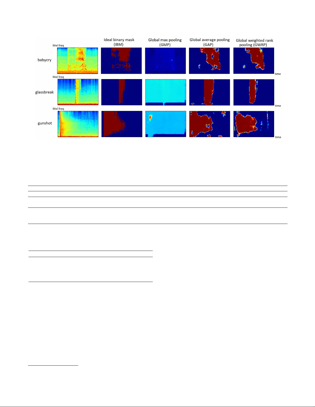
A JOINT SEP ARA TION-CLASSIFICA TION MODEL FOR SOUND EVENT DETECTION OF WEAKL Y LABELLED D A T A Qiuqiang K ong*, Y ong Xu*, W enwu W ang, Mark D. Plumble y Center for V ision, Speech and Signal Processing, Univ ersity of Surrey , UK {q.kong, yong.xu, w .wang, m.plumbley}@surrey .ac.uk ABSTRA CT Source separation (SS) aims to separate indi vidual sources from an audio recording. Sound ev ent detection (SED) aims to detect sound e vents from an audio recording. W e propose a joint separation-classification (JSC) model trained only on weakly labelled audio data, that is, only the tags of an au- dio recording are known b ut the time of the ev ents are un- known. First, we propose a separation mapping from the time-frequency (T -F) representation of an audio to the T -F segmentation masks of the audio e vents. Second, a classifi- cation mapping is built from each T -F segmentation mask to the presence probability of each audio event. In the source separation stage, sources of audio e vents and time of sound ev ents can be obtained from the T -F segmentation masks. The proposed method achieves an equal error rate (EER) of 0.14 in SED, outperforming deep neural network baseline of 0.29. Source separation SDR of 8.08 dB is obtained by using global weighted rank pooling (GWRP) as probability mapping, out- performing the global max pooling (GMP) based probability mapping gi ving SDR at 0.03 dB. Source code of our work is published. Index T erms — Sound e vent detection, source separation, weakly labelled data. 1. INTR ODUCTION Sound e vent detection (SED) aims to detect specific audio ev ents from an audio recording. SED has many applications in our daily life, for e xample, detecting a baby cry at home, detecting the tapping sound in an of fice and monitoring the fire alarm or gunshot [1] in a public area. On the other hand, source separation (SS) aims to separate individual sources from a recording [2] and can be used in SED [3]. Many current SED models are trained using supervised learning methods [4, 5, 6]. These supervised learning meth- ods need labelled onset and of fset time of the audio e vents, which we call str ongly labelled data (SLD). Labelling the SLD is time consuming and difficult to scale [4]. In addition, the onset and of fset time of some audio e vents are ambigu- ous due to the fade in and fade out effect, for e xample, the * The authors contribute equally to this work. approaching and moving away of a car . In contrast to the SLD, many audio datasets contain only the tags, that is, the presence or absence of audio e vents in an audio recordings. This is referred to as weakly labelled data (WLD) [7]. Many audio tagging datasets are weakly labelled [8, 9, 10] and are often larger than strongly labelled SED datasets [4, 9]. T o utilize the WLD, some methods including joint detection- classification (JDC) model [11], attention and localization model [12] and multi-instance learning methods [7] have been used. Source separation can be used for sound ev ent detection [3]. Unsupervised source separation methods in- cluding computation audio scene analysis (CASA) uses time- frequency (T -F) masking to emulate how human performs source separation [13]. Supervised source separation meth- ods need clean sources for training [2] and hav e achiev ed state-of-the-art performance. In this paper , a joint separation-classification (JSC) model is proposed to train the source separation model on the WLD. The proposed framework consists of two parts. The first part is a separation mapping from the T -F represen- tation of an audio signal to the T -F segmentation masks of each audio e vent. The second part is a classification mapping from each se gmentation mask to its corresponding audio tag. In the source separation stage, separated sources of different classes can be obtained from the T -F segmentation masks. The remainder of the paper is organized as follows: Sec- tion 2 discusses con volutional neural netw ork. Section 3 pro- poses the source separation frame work. Section 4 shows e x- perimental results. Section 5 concludes and proposes the fu- ture work. 2. CONV OLUTION AL NEURAL NETWORK Con volutional neural networks (CNNs) are used initially in image classification [14] and recently ha ve been very success- ful in audio processing, including speech recognition and au- dio classification [15]. In audio classification, the waveform is transformed to T -F representations which are treated as an image and fed as input to a CNN [15]. A CNN consists of sev eral con v olutional layers and each contains sev eral train- able filters trained to learn some local patterns in the feature map. Downsampling usually follo ws some con v olutional lay- Wa veform T-F representa tion Segmentation masks × T r aining g 1 x ( , ) X t f ( , ) h t f Phase Segmentation masks Audio tags Inverse T-F representa tion Separated w aveform × g 2 ( , ) k h t f k y , 1 , ..., k x k K  ^ k X h  Fig. 1 . Framew ork of the joint separation-classification model. ers to reduce the size of the feature maps. Finally a global max pooling on each feature map [15] is usually used to se- lect the most prominent T -F unit in each feature map followed by a fully connected neural network for classification [15]. 3. PR OPOSED JOINT SEP ARA TION-CLASSIFICA TION MODEL In this section, a joint separation-classification (JSC) model trained on WLD is proposed. This idea is related to the ob- ject localization from weakly labelled images [16, 17], where only the labels of an image are kno wn, but the location of the objects are unknown. In [16] a class acti v ation mapping (CAM) is applied to highlight the class-specific discrimina- tiv e regions to localize objects from weakly labelled data. Similar to the weakly labelled image data [16, 17], many audio datasets [4] only contain the tags of an audio recording, but the happening time of the e vents are unkno wn. The pro- posed separation-classification model is sho wn in Fig. 1. The input audio wa veform x is transformed to a time-frequency (T -F) representation X ( t, f ) such as a spectrogram or log Mel spectrogram. T o simplify the notation we abbre viate X ( t, f ) as X . The first part of the model is a separation mapping g 1 : X 7→ h from the input T -F representation X to the T -F segmentation masks h = [ h 1 , ..., h K ] , where K is the num- ber of audio tags and h k is the T -F segmentation mask of the k -th audio tag. The values on each segmentation mask are be- tween 0 and 1 for source separation. The mapping g 1 can be parametrized by trainable parameters. The second part of the model is a classification mapping g 2 : h k 7→ y k , k = 1 , ..., K from each segmentation mask to its corresponding audio tag, where y k ∈ [0 , 1] represents the presence probability of the k -th ev ent in an audio recording. A compound model g 2 ◦ g 1 is a mapping from the input T -F representation X to the audio tags y k , k = 1 , ..., K . In the training phase, the model can be trained end-to-end from X to y k , k = 1 , ..., K . In the sep- aration stage, the T -F representation of an input wa veform is passed through the mapping g 1 to get the segmentation masks. Then the input T -F representation is multiplied by each seg- mentation mask to obtain the separated T -F representation of each ev ent with corresponding audio tag. Then an in verse T -F transform is applied on each separated T -F representation of each audio tag using the phase of the original wa veform to obtain its separated wav eform of each audio tag (Fig. 1). Fi- nally , SED result of each audio ev ent can be obtained from its corresponding segmentation masks. 3.1. Separation mapping W e apply log Mel spectrogram as input T -F representation, which is a good representation for audio tagging [15]. W e apply a CNN to model the separation mapping g 1 . The CNN modeled JSC model is sho wn in Fig 2. W e remove all the downsampling layers to keep the resolution of each T -F seg- mentation mask the same as the input T -F representation. This high resolution T -F segmentation mask is useful for source separation. The number of feature maps in the last conv olu- taional layer is the sam e as the number of audio e v ents to sep- arate followed. Then a sigmoid nonlinearity is applied on the feature maps to obtain the segmentation to ensure the v alues on segmentation masks are between 0 and 1. This segmen- tation mask of this T -F representation is similar to the class activ ation mapping (CAM) in weak image localization [16]. 3.2. Classification mapping The classification mapping g 2 maps each segmentation mask to the presence probability of its corresponding tag. Classifi- cation mapping can be modeled by , for example, global max pooling (GMP) [16], global average pooling (GAP) [18, 16] or global weighted rank pooling (GWRP) [19]. 3.2.1. Global max pooling Global max pooling (GMP) [15] is defined as follows: g ( h c ) = max t,f h c ( t, f ) (1) where h c represents the c -th segmentation mask and t , f are index es of time and frequency bin. GMP returns the highest value on each feature map. GMP performs well in classifica- tion b ut tends to underestimate the T -F units of e vents in each segmentation mask [16] because only the T -F unit with the highest value is passed to the ne xt layer (Fig. 3). 3.2.2. Global averag e pooling Global av erage pooling (GAP) [18] is defined as: g ( h c ) = 1 M X t,f h c ( t, f ) (2) Fig. 2 . Con v olutional neural network (CNN) based weak source separation. Log Mel spectrogram is used as T -F representation. Separation mapping is modeled by a CNN. Classification mapping is applied on each T -F segmentation mask to obtain the prediction of audio tags. In separation stage, the separated wav eforms are obtained from the segmentation masks. where M is the number of time frames multiplied number of frequency bins. In contrast to GMP , GAP averages all the values of T -F units on a segmentation mask, which tends to ov erestimate the ev ents in a segmentation mask [19] (Fig. 3). 3.2.3. Global weighted rank pooling Global weighted rank pooling (GWRP) is proposed in [19] and is a generalization of GMP and GAP . Define I c = { i 1 , ...i n } as an inde x set in descending order of the v al- ues on feature map h c , i.e. ( h c ) i 1 ≥ ( h c ) i 2 ≥ ... ≥ ( h c ) i n . Then GWRP is defined as g ( h c ) = 1 Z ( d c ) N X j =1 ( d c ) j − 1 ( h c ) i j (3) where 0 ≤ d c ≤ 1 is a hyper parameter and N = T F is the number of T -F units in a segmentation mask and Z ( d c ) = P N j =1 ( d c ) j − 1 is a normalization term. When d c = 0 and d c = 1 , GWRP simplifies to GMP and GAP , respectiv ely . 3.3. Sound event detection The segmentation masks obtained from the JSC model con- tains the presence of the audio ev ents in a T -F representation (Fig 3). Hence we achieved sound ev ent segmentation in T -F domain. In this paper we simply average out the frequency axis to obtain the SED in the time axis. 4. EXPERIMENTS In this section we apply the proposed JSC model on the mod- ified detection of rare audio sound e vents dataset from T ask 2 of DCASE 2017 challenge [10]. This dataset consists of rare e vents including “babycry”, “gunshot” and “glassbreak”. The background sounds come from the acoustic scene dataset from T ask 1 of the DCASE 2017 data challenge [10]. T o in- vestigate WLD, we extract se veral rare audio e vents from the dataset and mix the rare audio ev ents with 4 second clips from the acoustic scene dataset. Altogether 1008 clips are created for training, with 1/3 are single labelled and 2/3 are multil- abelled. Only the presence or absence of the audio e vents in an audio clip is known. The audio mixtures are conv erted to monaural, and the sampling rate is 16 kHz. A log Mel spec- trograms with 64 frequency bins are used as the T -F represen- tation. In the Fourier transform a Hamming window with size of 1024 and ov erlap of 280 samples is used to ensure that there are 128 frames in each 4 seconds clip. W e apply a V isual Ge- ometry Group [14] like CNN consists of 8 conv olutional lay- ers. Each layer consists of 64 feature maps follo wed by batch normalization (BN) [20] and ReLU nonlinearity . Dropout rate of 0.3 is applied to regularize overfitting. The value of d c in GWRP is set as 0.999. These hyper-parameters are chosen empirically , but they do not af fect the result much. The learned se gmentation masks using dif ferent classifi- cation mappings are visualized in Fig 3. The first column shows the log Mel spectrogram of a “babycry”, a “glassbreak” and a “gunshot”. The second column shows the ideal binary mask (IBM) [21] of the audio ev ents. Column 3 to 5 shows the segmentation masks learned using GMP , GAP and GWRP as classification mapping, respecti vely . It can be observed that GMP tends to underestimate the presence of the audio ev ents in the T -F segmentation mask. GAP and GWRP performs better in learning the T -F segmentation mask on this dataset. T able 1 shows the separation results of different audio tags ev aluated on SDR, SIR and SAR [22]. The results of IBM [21] and without separation are listed as baselines. GWRP performs better in terms of SDR and SAR in babycry , glass- break, gunshot and background than without separation, GMP and GAP . T able 1 shows that source separation using the pro- posed JSC model outperforms significantly the baseline with- out separation. T able 1 also sho ws how far JSC is from the Fig. 3 . V isualization of the segmentation masks using different global pooling strategy . The first column sho ws the log Mel spectrogram of babycry , glassbreak and gunshot sound in noisy background. The second column shows the ideal binary mask. The third to the fifth column shows the T -F segmentation masks learned using global max pooling (GMP), global av erage pooling (GAP) and global weighted rank pooling (GWRP), respectiv ely . T able 1 . Separation results of mixed rare e vents with background sound using dif ferent methods. Babycry Glassbreak Gunshot A vg. SDR SIR SAR SDR SIR SAR SDR SIR SAR SDR SIR SAR w/o separation -3.66 -3.66 inf -7.52 -7.52 inf -6.48 -6.48 inf -5.89 -5.89 inf IBM 20.14 34.73 20.32 18.62 37.35 18.70 15.24 33.04 15.35 18.00 35.04 18.12 Proposed GMP 2.99 15.43 5.85 -1.79 0.79 10.05 -1.11 1.66 9.84 0.03 5.96 8.58 Proposed GAP 9.58 22.61 10.21 6.35 17.81 8.49 2.25 13.05 4.73 6.06 17.82 7.81 Proposed GWRP 13.36 24.61 14.20 12.29 28.06 12.86 -1.41 13.93 -0.28 8.08 22.20 8.93 T able 2 . Frame wise equal error rate (EER) of mix ed rare ev ents with background sound using dif ferent method. babycry glassbreak gunshot a vg. baseline DNN 0.27 0.26 0.34 0.29 weak GMP 0.27 0.30 0.32 0.30 weak GAP 0.11 0.12 0.19 0.14 weak GWRP 0.11 0.10 0.20 0.14 IBM in source separation. T able 2 shows the frame wise sound ev ent detection equal error rate (ERR) using different global pooling strategies. GAP and GWRP outperforms the baselines DNN and GMP . The results are correspondent to the visualization of segmen- tation masks in Fig 3. and T able 1. W e published source code of our work 1 . 1 https://github .com/qiuqiangkong/ICASSP2018_joint_separation_classification 5. CONCLUSION In this paper a joint separation-classification (JSC) model has been presented for sound event detection and source separa- tion. A separation mapping from the input time-frequency representation to the segmentation masks and a classification mapping from each segmentation mask to each audio tag are proposed. W e obtain frame wise sound ev ent detection EER of 0.14, which outperforms the DNN baseline, and a verage source separation SDR of 8.08 using global weighted rank pooling compared to SDR of 0.03 using global max pooling. In future, we will research more on improving the source sep- aration quality using the JSC model. 6. A CKNO WLEDGEMENT This research is supported by EPSRC grant EP/N014111/1 “Making Sense of Sounds” and research scholarship from the China Scholarship Council (CSC). Thank to Sacha Krstulovic, Giacomo Ferroni and Adrian Stepien from Audio Analytic Ltd for discussions on audio ev ent detection. 7. REFERENCES [1] G. V alenzise, L. Gerosa, M. T agliasacchi, F . Antonacci, and A. Sarti, “Scream and gunshot detection and local- ization for audio-surveillance systems, ” in IEEE Confer- ence on Advanced V ideo and Signal Based Surveillance, 2007 . IEEE, 2007, pp. 21–26. [2] P . Huang, M. Kim, M. Hasegawa-Johnson, and P . Smaragdis, “Deep learning for monaural speech sepa- ration, ” in IEEE International Confer ence on Acoustics, Speech and Signal Pr ocessing (ICASSP) . IEEE, 2014, pp. 1562–1566. [3] T . Heittola, A. Mesaros, T . V irtanen, and A. Eronen, “Sound e vent detection in multisource en vironments us- ing source separation, ” in Machine Listening in Multi- sour ce En vir onments , 2011. [4] A. Mesaros, T . Heittola, and T . V irtanen, “TUT database for acoustic scene classification and sound event detec- tion, ” in EUSIPCO . IEEE, 2016, pp. 1128–1132. [5] D. Stowell, D. Giannoulis, E. Benetos, M. Lagrange, and M. D. Plumbley , “Detection and classification of acoustic scenes and ev ents, ” IEEE T ransactions on Mul- timedia , vol. 17, no. 10, pp. 1733–1746, 2015. [6] T . Heittola, A. Mesaros, A. Eronen, and T . V irtanen, “Context-dependent sound e vent detection, ” EURASIP Journal on Audio, Speec h, and Music Pr ocessing , vol. 2013, no. 1, pp. 1, 2013. [7] A. Kumar and B. Raj, “ Audio ev ent detection using weakly labeled data, ” in Proceedings of the 2016 ACM on Multimedia Conference . ACM, 2016, pp. 1038– 1047. [8] P . Foster , S. Sigtia, S. Krstulovic, J. Barker , and M. D. Plumbley , “CHiME-home: A dataset for sound source recognition in a domestic en vironment, ” in IEEE W ork- shop on Applications of Signal Pr ocessing to Audio and Acoustics (W ASP AA) . IEEE, 2015, pp. 1–5. [9] J. F . Gemmeke, D. P . W . Ellis, D. Freedman, A. Jansen, W . Lawrence, R. C. Moore, M. Plakal, and M. Ritter, “Audio Set: An ontology and human-labeled dataset for audio ev ents, ” in IEEE ICASSP , 2017, pp. 776–780. [10] A. Mesaros, T . Heittola, A. Diment, B. Elizalde, A. Shah, E. V incent, B. Raj, and T . V irtanen, “DCASE 2017 challenge setup: T asks, datasets and baseline sys- tem, ” in Pr oceedings of the Detection and Classifica- tion of Acoustic Scenes and Events (DCASE) W orkshop , 2017. [11] Q. K ong, Y . Xu, W . W ang, and M. D. Plumbley , “ A joint detection-classification model for audio tagging of weakly labelled data, ” in IEEE International Con- fer ence on Acoustics, Speech and Signal Pr ocessing (ICASSP) . IEEE, 2017, pp. 641–645. [12] Y . Xu, Q. K ong, Q. Huang, W . W ang, and M. D. Plumb- ley , “ Attention and localization based on a deep con- volutional recurrent model for weakly supervised audio tagging, ” arXiv pr eprint arXiv:1703.06052 , 2017. [13] D. W ang and G. J. Brown, Computational Auditory Scene Analysis: Principles, Algorithms, and Applica- tions , W ile y-IEEE press, 2006. [14] K. Simonyan and A. Zisserman, “V ery deep con vo- lutional netw orks for large-scale image recognition, ” arXiv pr eprint arXiv:1409.1556 , 2014. [15] K. Choi, G. Fazekas, and M. Sandler , “ Automatic tag- ging using deep conv olutional neural networks, ” arXiv pr eprint arXiv:1606.00298 , 2016. [16] B. Zhou, A. Khosla, A. Lapedriza, A. Oliv a, and A. T or- ralba, “Learning deep features for discriminative lo- calization, ” in Pr oceedings of the IEEE Confer ence on Computer V ision and P attern Recognition , 2016, pp. 2921–2929. [17] M. Oquab, L. Bottou, I. Lapte v , and J. Si vic, “Is ob- ject localization for free?-weakly-supervised learning with conv olutional neural networks, ” in Pr oceedings of the IEEE Confer ence on Computer V ision and P attern Recognition , 2015, pp. 685–694. [18] M. Lin, Q. Chen, and S. Y an, “Network in network, ” arXiv pr eprint arXiv:1312.4400 , 2013. [19] A. Kolesnik ov and C. H. Lampert, “Seed, expand and constrain: Three principles for weakly-supervised im- age segmentation, ” in Eur opean Confere nce on Com- puter V ision . Springer , 2016, pp. 695–711. [20] S. Ioffe and C. Szegedy , “Batch normalization: Accel- erating deep netw ork training by reducing internal co- variate shift, ” in International Confer ence on Machine Learning , 2015, pp. 448–456. [21] D. W ang, “On ideal binary mask as the computational goal of auditory scene analysis, ” Speech Separation by Humans and Machines , pp. 181–197, 2005. [22] E. V incent, R. Gribon v al, and C. Févotte, “Performance measurement in blind audio source separation, ” IEEE T r ansactions on Audio, Speech, and Language Pr ocess- ing , vol. 14, no. 4, pp. 1462–1469, 2006.