A Novel Hybrid Scheme Using Genetic Algorithms and Deep Learning for the Reconstruction of Portuguese Tile Panels

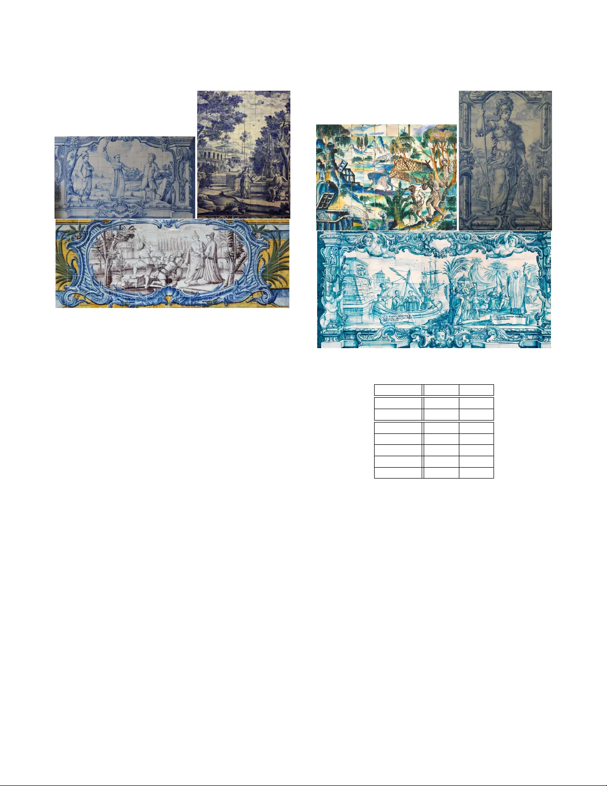
A No vel Hybrid Scheme Using Genetic Algorithms and Deep Learning f or the Reconstruction of P or tuguese Tile P anels Daniel Rika Dept. of Computer Science Bar-Ilan Uni versity Ramat-Gan 52900, Israel danielrika@gmail.com Dror Sholomon Dept. of Computer Science Bar-Ilan Uni versity Ramat-Gan 52900, Israel dror .sholomon@gmail.com Eli (Omid) David Dept. of Computer Science Bar-Ilan Uni versity Ramat-Gan 52900, Israel mail@elidavid.com Nathan S. Netanyahu * Dept. of Computer Science Bar-Ilan Uni versity Ramat-Gan 52900, Israel nathan@cs.biu.ac.il ABSTRA CT This paper presents a nov el scheme, based on a unique combina- tion of genetic algorithms (GAs) and deep learning (DL), for the automatic reconstruction of P ortuguese tile panels , a challenging real-world variant of the jigsaw puzzle problem (JPP) with impor- tant national heritage implications. Specifically , we introduce an enhanced GA-based puzzle solv er , whose integration with a nov el DL-based compatibility measur e (DLCM) yields state-of-the-art per- formance, regarding the above application. Current compatibility measures consider typically (the chromatic information of) edge pixels (between adjacent tiles), and help achie ve high accuracy for the synthetic JPP variant. Howe ver , such measures exhibit rather poor performance when applied to the Portuguese tile panels, which are susceptible to various real-world effects, e.g., monochromatic panels, non-squared tiles, edge degradation, etc. T o ov ercome such difficulties, we ha ve de veloped a no vel DLCM to extract high-le vel texture/color statistics from the entire tile information. Integrating this measure with our enhanced GA-based puzzle solver , we have demonstrated, for the first time, how to deal most effecti vely with large-scale real-world problems, such as the Por- tuguese tile problem. Specifically , we have achie ved 82% accuracy for the reconstruction of Portuguese tile panels with unknown piece rotation and puzzle dimension (compared to merely 3.5% a verage ac- curacy achie ved by the best method known for solving this problem variant). The proposed method outperforms ev en human experts in sev eral cases, correcting their mistakes in the manual tile assembly . KEYWORDS Real W orld Applications, Genetic Algorithm, Reconstruction, Deep Learning, Jigsaw Puzzle Problem, Portuguese T ile Panels 1 INTR ODUCTION Object reconstruction from numerous fragments is a perv asiv e, im- portant task that has been encountered in many areas throughout * Also affiliated with the Gonda Brain Research Center at Bar-Ilan Uni versity , and the Center for Automation Research, Univ ersity of Maryland, College Park, MD 20742. Figure 1: Reconstruction of Portuguese tile panels with un- known piece orientation and panel dimensions, due to our pr o- posed system. Left: Input images of Portuguese tile panels, con- taining 256 (top) and 150 (bottom) pieces. Right: Perfectly r e- constructed images due to our novel compatibility measure cou- pled with the enhanced version of a "kernel-gro wth" GA. human civilization. Piecing together brok en pottery , ancient fres- coes, or shredded documents from their artifacts are merely a few examples. The most basic generic version of the problem is to as- semble an object from its n different (non-overlapping) pieces as Ref: ACM Genetic and Evolutionary Computation Confer ence (GECCO) , pages 1319-1327, Prague, Czech Republic, July 2019. GECCO ’19, July 13–17, 2019, Prague, Czech Republic D . Rika, D . Sholomon., E.O . David, and N.S. Netany ahu accurately and efficiently as possible. (T o automate this challenging task, processing is often applied to colored images acquired from these pieces.) The basic problem definition is very similar to the popular jigsaw puzzle pr oblem (JPP), which is known to be NP com- plete [ 1 , 11 ]. The JPP has been pursued by many researchers, as it is a special instance of a broad class of challenging real-world problems, such as image editing [ 6 ], the recov ery of shredded doc- uments or photographs [ 10 , 19 , 24 , 27 ], art conserv ation [ 2 , 4 , 21 ], speech descrambling [ 7 , 51 ], etc., as well as additional problems in areas like biology [ 26 ], chemistry [ 46 ], literature [ 28 ], and more. Obviously , there are notable differences, in practice, between a pure JPP setting and the above real-world problems ( e .g. unknown di- mensions, missing pieces, gaps between pieces due to degradation ov er time, pieces from multiple puzzles, etc.). Nev ertheless, the JPP serves as a testbed for developing ground-breaking methods for these important challenges. Every reconstruction procedure requires a compatibility measur e to estimate the likelihood that two given pieces are adjacent and a strategy for placing the pieces as “accurately” as possible with respect to some global objective function. Although much effort has been dev oted to devising reliable compatibility measures for jigsa w- like problems, they may not alw ays be consistent 1 ; if they were, the problem would not be NP-hard. More importantly , the typical de- pendence of current compatibility measures on correlations between low-le vel color/texture statistics in the proximity of tile boundaries, renders jigsaw puzzle solvers based on such measures virtually ineffecti ve for real-world problems, such as the reconstruction of archaeological fragments and shredded documents (where often the information is sev erely degraded near the points of fraction), or that of Portuguese tile panels, whose image content is not necessarily color-rich and where chromatic information near tile boundaries might be sev erely corrupted. In addition, many methods for solving optimally the piece placement problem resort to greedy strategies, which are problematic in encountering local optima. Moreov er , they usually cannot recover from erroneous placements made early on (as a result of a greedy , locally optimal choice). T o meet these chal- lenges, we employ in this paper a computational intelligence (CI) approach in dealing ef fectiv ely with both components of the prob- lem ( i.e. the search and the compatibility measure). Specifically , we present a unique combination of: (1) An enhanced genetic algo- rithm (GA)-based scheme for finding promising (partial) solutions ( i.e. fittest chr omosomes ), at each iterative stage, as a strategy for optimal piece placement, and (2) a novel deep learning (DL) model for learning piece compatibility by directly training on the raw data (of a fairly small training set), without applying an y standard feature selection/extraction techniques, Our contributions are summarized as follo ws: (1) Provided an enhanced GA solv er for the construction of Por- tuguese tile panels; (2) Obtained for the first time a DL-based compatibility measure (DLCM) for a real-world JPP-like task; 1 In the sense that the most compatible piece to a given piece A , with respect to a compatibility measure in question, may not necessarily be adjacent to A in the “correct” puzzle configuration. (3) Presented a unique combination of the above GA module and the novel compatibility measure for the reconstruction of Portuguese tile panels on a large-scale basis (see e.g . Fig. 1); (4) Obtained state-of-the-art-results for the above real world problem; specifically , achiev ed an av erage accuracy of 82% on T ype 2 puzzles with unknown dimensions (compared to merely 3.5% a verage accuracy achieved by Gallagher’ s method [ 16 ], which is the best method kno wn for solving this problem variant); (5) Compiled a new benchmark for the community , regarding training and test data for the Portuguese tile problem. The paper is organized as follo ws. Section 2 provides a brief surve y of recent related work. Section 3 and Section 4 describe, respectiv ely , our nov el GA-based solv er and the DL method for learning a compatibility measure. Section 5 presents the datasets used, and Section 6 pro vides detailed experimental results. Section 7 makes concluding remarks. 2 RELA TED WORK 2.1 Synthetic JPP 2.1.1 T raditional Methods. Freeman and Garder [ 15 ] intro- duced initially in 1964 a computational solver , which handled up to nine-piece puzzles. Subsequent research [ 17 , 22 , 35 , 48 ] relied solely on shape cues of the pieces. K osiba et al. [ 23 ] were the first to use image content, in addition to boundary shape; their method computes color compatibility along the matching contour , rew arding adjacent jigsaw pieces with similar colors. This trend continued for more than a decade (see, e.g . [ 8 , 25 , 29 , 37 , 50 ]), before the research focus shifted from shape-based to merely color -based solvers of square-tile puzzles with known piece orientation ( i.e . T ype 1 puzzles). Cho et al. [ 5 ] used dissimilarity ( i.e. the sum, ov er all neighboring pixels, of squared color differences o ver all color bands), as a compat- ibility measure for their probabilistic puzzle solver , that handles up to 432 pieces, gi ven some a priori kno wledge of the puzzle. (The sum of squared differences is referred to as SSD.) Their 2010 paper w as followed by Y ang et al. [ 49 ], who reported improv ed performance due to their particle filter -based solver . Shortly after, Pomeranz et al. [ 34 ] presented, for the first time, a fully-automated jigsaw puzzle solver of puzzles containing up to 3,000 square pieces, using the abov e defined dissimilarity and their so-called best-b uddies heuristic. Gallagher [ 16 ] adv anced further the state-of-the-art by considering a more general variant of the problem, where a piece orientation is unknown ( i.e. T ype 2 puzzle), as well as the puzzle dimensions. Specifically , he presented the preferable measure of Mahalanobis gradient compatibility (MGC), which penalizes changes in intensity gradients (rather than changes in intensity) and learns the co variance of the color channels, using the Mahalanobis distance. He suggested also dissimilarity ratios for a more indicativ e compatibility measure. Sholomon et al. [ 40 – 42 ] pursued a GA-based approach based on a number of innov ativ e cr ossover procedures, and demonstrated the effecti ve performance of their methodology on very lar ge T ype 1 and T ype 2 puzzles (including two-sided puzzles and a number of mixed puzzles). Son et al. [ 45 ] imposed so-called loop constraints , where the dissimilarity ratio (with respect to the smallest distance from a piece edge in question), for each consecuti ve pair of pieces along a loop of four or more pieces, is below a certain threshold. They were A Nov el Hybrid Scheme Using Genetic Algorithms and Deep Learning for the Reconstr uction of P or tuguese Tile Panels GECCO ’19, July 13–17, 2019, Prague, Czech Republic able to improve the accuracy for both T ype 1 and T ype 2 puzzles in certain cases. Also, they pro vided, for the first time, an upper bound on the reconstruction accuracy for various datasets. Paikin and T al [ 31 ] proposed a greedy solv er based on an asymmetric L 1 - norm dissimilarity and the best-b uddies heuristic. They demonstrated how to handle, among other things, puzzles with missing pieces, and reported improved accuracy results and fast running times. More recently , Andaló et al. [ 3 ] showed how to map the JPP to the problem of maximizing a constrained quadratic function, and presented a deterministic algorithm for solving it via gradient ascent. 2.1.2 DL Methods. Recently , there have been also a fe w DL works related to the JPP [ 12 , 13 , 30 , 38 ]. Ho wev er , these works barely provide an y practical solutions to e ven “toy instances” of the JPP , and their main thrust is to “re-purpose” a neural network, trained to solve a simple jigsaw puzzle (without manual labeling), to handle adv anced tasks, such as object detection and classification, in an unsupervised manner . Other than the above, a DL-based heuristic called DNN-buddies was presented in [ 43 ], in an attempt to enhance the accuracy of a GA-based solv er . It should be noted, though, that the abov e heuristic is employed in conjunction with the SSD mea- sure, in a rather restricti ve manner , so it is expected to perform rather poorly on real-world JPP-like tasks. 2.2 Real-W orld Portuguese Tile Panels The reconstruction of ancient frescoes and w all paintings from nu- merous lar ge repositories of fragmented artifacts, compiled over time due to natural deterioration, is of utmost importance in preserv- ing world cultural heritage. V arious ef forts to automate the process ( e.g . [ 4 , 33 , 44 ]) rely primarily on shape matching (in 2D and 3D) of fragments followed by their assembly . While exhibiting good perfor- mance on relativ ely small datasets (only a fe w hundred fragments), the scalability of these efforts (in terms of the number of fragments and the number of art works in a gi ven pool) is questionable. Our focus in this paper is on the reconstruction of the Portuguese tiles panels [ 9 ], which concerns the assembly of ancient panels of 2D square tiles that have been removed from many buildings and landmarks in Portugal (see Figure 2). Currently , over one hundred thousand such tiles are stored at the Portuguese National Tile Mu- seum (Museu Nacional do Azulejo) in Lisbon, and are awaiting manual assembly by human experts. In view of the extremely chal- lenging nature of the problem, it would tak e decades, at the current pace, before all these “jigsaw puzzles” are solved, i.e. before the panels are assembled by the human experts [32]. Fonseca [ 14 ] acquired tile images and adapted their shape to squares; he then applied an augmented Lagrange multipliers tech- nique to an equiv alent optimization problem and a greedy approach for T ype 1 and T ype 2 v ariants, respectiv ely . He obtained 57.8% and 39.1% accuracy for these cases, respectiv ely , on panels contain- ing only a fe w dozen tiles. In comparison, Gallagher’ s method [16] achiev es corresponding accuracy lev els of 64.5% and 49.4%. An- dalo et al. [ 2 ] reported perfect reconstruction (of 4 mixed tile panels) using their PSQP method [ 3 ] for known tile orientation. Howe ver , their method does not handle the T ype 2 variant, and its preliminary results were obtained for panels containing a fairly small number of, presumably , high-resolution tiles. Figure 2: Manual assembling of a panel of Portuguese tiles at the National Tile Museum (Museu Nacional do Azulejo, MNAz), Lisbon, Portugal: Source [14]. 3 GA SOL VER W e seek a global optimizer that can exploit the relati ve accurate piece adjacency prediction capability , but that can also overcome its inaccuracies. Previous solv ers rely typically on some specialized criterion, which implies a subset of edge adjacencies that are likely to be correct. T o av oid searching for such a specific criterion, we pursue a GA approach [ 18 ] for tile placement, in the spirit of the kernel-gr owth scheme presented in Sholomon et al. [ 40 , 41 ]. Since the proposed GA solver is of a random nature, it could correct, potentially , wrong adjacencies during the global optimization. Follo wing [ 40 ], we describe here the new hierarchical phases of our modified cr ossover operator . In a nutshell, a chromosome is associated with a puzzle configuration (or a “solution”), and its fitness function is defined by the o verall sum of pairwise, adjacent tile compatibilities (see below). The principle of hierarchical phases is that a piece is added to the gro wing kernel at each phase only if the previous phases hav e been exhausted ( i.e . no further pieces can be added due to these phases); the crossover terminates once the kernel contains all the pieces. Our proposed phases and their hierarchical arrangement are as follows. • Phase I: If there is a free (piece) boundary in the kernel, which has a neighboring piece in a chromosome parent, such that the score of each of these adjacent pieces is greater than max ( 0 . 8 , C mean ) , where C mean is the chromosome’ s average compatibility across all boundaries, then add the neighboring piece to the k ernel. W e define the score of a piece as the av erage compatibility measure between the piece and all of its neighbors. This phase gives priority to the chromosome parent with the higher fitness, assuming that it would yield a more accurate reconstruction rate. • Phase II: Similar to Phase I, except that this phase selects the chromosome parent with the lower fitness. • Phase III: If there is a free (piece) boundary in the kernel, such that the two chromosome parents agree on the adjacent piece, place this piece next to the boundary in question. • Phase IV : If there is a free (piece) boundary in the kernel, such that its most compatible piece is available ( i.e. is not placed already in the kernel), then add that compatible piece to the kernel. GECCO ’19, July 13–17, 2019, Prague, Czech Republic D . Rika, D . Sholomon., E.O . David, and N.S. Netany ahu • Phase V : If there is a free (piece) boundary in the kernel, such that its second-most compatible piece is av ailable, then add the latter piece to the kernel. • Phase VI: Pick randomly one of the remaining pieces, and place it randomly at one of the free boundaries of the kernel. W e introduce a certain de gree of randomness to the process (known as mutation ), in order to av oid local maxima, by skipping some of the crossover phases, with small probability . Specifically , we skip the first and second phases with 10% probability and the third phase with 20% probability . The other phases are always ex ecuted. Other hyper-parameters of our modified GA solver (which were arriv ed at after exhausti ve experimentation) are as follows: Chro- mosomes are chosen for the crossover operation according to the r oulette wheel selection , the population consists of 100 chromo- somes, and the GA runs for 500 generations. 3.1 Rationale Before explaining the rationale behind the above phases, we note that our proposed crossover does not draw on the notion of best- buddies , as w as defined and used e.g . in [ 34 ] and [ 40 ]. The reason for that is that in contrast to the (synthetic) JPP , where best-b uddy pairs were found to be adjacent with 95% probability , our e xperience with the Portuguese tile panels shows that best-buddy pairs, with respect to our state-of-the-art DLCM (described in the next section), are correct with only 70% probability . Regarding our modified crossov er operator , note that the objecti ve of the first and second phase is to inherit correctly-reconstructed segments from the parents. W e constrain the score of each of the two pieces in question to be at least 0.8, as a good starting threshold. (Note that the score is in the range between 0 to 1, due to the nor- malization of the compatibility measure as explained in Sec. 4.3.) Furthermore, since the algorithm improves as the number of gen- erations goes up, ( i.e. chromosome fitness increases), the resulting threshold becomes greater than 0.8. The idea behind the dynamic threshold, is to ov ercome errors made in pre vious generations. Phase III is carried out if the two chromosomes agree on the same pair of pieces, i.e. the y are likely to be correct, with high probability . In the first three phases the crosso ver inherits adjacent pieces from the parents; howe ver , these phases might not necessarily result in a successful addition of a new piece to the kernel. Thus, Phases IV and V , which rely solely on our proposed DLCM, could be used alternativ ely by considering the most compatible and second-most compatible pieces. If Phases IV and V still fail to add one more piece to the kernel (because the pieces considered are already placed in the kernel), Phase VI is in voked to complete the puzzle configuration, by placing randomly a free piece at an open boundary . 4 TRAINING A COMP A TIBILITY MEASURE W e hav e striv en to dev elop a DL model for learning automatically a compatibility measure, such that gi ven two puzzle pieces, it would distinguish between adjacent and non-adjacent pieces. The proposed method is based loosely on ideas from the field of metric embed- ding learning . The goal of metric embedding learning is to learn a function f θ ( x ) : R F → R D , which maps semantically similar points from the data manifold R F onto metrically close points in R D . This approach was first presented by W einberger and Saul [ 47 ], in the context of nearest-neighbor classification. Schroff et al. [ 39 ] subsequently proposed using a deep con volutional neural network (CNN)-based embedding of human f aces, which is trained via a so-called triplet-loss described below . W e propose to formulate the problem of learning a compatibility measure as learning a single-dimensional embedding E × E → R , where E is the group of all puzzle piece edges. Here we want to ensure that giv en a piece-edge e i (anchor) and its adjacent piece- edge e j in the original image, the score of the positive pair ( e i , e j ) will be higher than any ne gative pair ( e i , e k ) . This can be achie ved by minimizing the loss L = Õ e i , e j , e k ∈ T max ( 0 , 1 − f ( e i , e j ) + f ( e i , e k )) , where f is a deep con volutional neural network and T is the training set. 4.1 T riplet Selection Since the number of possible triplets in the training set is quite large, we generated the training triplets online. Specifically , we selected, for each epoch, 25 pieces at random from e very puzzle in our dataset. W e used the edges of each piece as anchors, generating positi ve pairs from each edge and its neighboring pieces. (Usually this results in four pairs, but could also result in three or two pairs only , for pieces along the puzzle boundaries and the four corner pieces, respecti vely .) For each such positi ve pair , we randomly select a non-adjacent piece edge and create its accompanying ne gativ e pair to form a triplet. Next, we randomly augmented each piece in each pair , using either de gradation or shifting . Degradation replaces randomly the outermost pixel frame of the piece with zeros. W ith uniform probabil- ity , we may replace no pixel, replace a pixel-wide frame, or replace a double pixel frame. This should aid the netw ork in learning more than only near-border textures. For shifting, we randomly shift the piece anywhere between zero to two pixels horizontally or v ertically (filling with zeros empty locations). Figure 3 demonstrates some possible outcomes. Figure 3: Illustration of tile augmentation via degradation and shifting. From left to right: Degraded tile by removing 2 pixels from its outer frame; shifted tile by one pixel to the left, and one pixel up; augmented tile with degradation and shifting. 4.2 Deep Conv olutional Neural Networks W e trained a deep con volutional neural network (CNN), which re- ceiv es as input a pair of puzzle pieces and returns a real number score. All pieces are of size 50 × 50 pixels. Although most actual A Nov el Hybrid Scheme Using Genetic Algorithms and Deep Learning for the Reconstr uction of P or tuguese Tile Panels GECCO ’19, July 13–17, 2019, Prague, Czech Republic puzzle pieces are lar ger , we do wnscaled them to better fit in memory and speed up the training phase. Always taking the anchor piece to be on the left, we rotate the pieces accordingly . For e xample, to compare the left edge of an anchor piece with the right edge of piece p , we would rotate both pieces by 180 ° , so that the anchor piece will still be on the left, but its left edge no w points to the right. During training we noticed that determining the degree of com- patibility for some pairs could be rather dif ficult for both the network and human experts, but it becomes quite easier for humans when looking only at a single color channel. Drawing on this observ ation, we trained the follo wing networks: Red-Net, Green-Net, and Blue- Net (named after the color channels each receiv es as input), as well as a fourth network, RGB-Net (which receiv es all three channels as input). All networks share the exact same architecture, as depicted in Figure 4. During training we presented all netw orks with the same batch ( i.e. same training samples); each network’ s loss was calcu- lated separately , so as not to affect the other networks. T able 2 gives a performance comparison, regarding the above indi vidual networks and their proposed combined scheme. W e trained all networks using stochastic gradient descent (SGD) with standard backpropagation [ 36 ] and Adam [ 20 ], using a learning rate of 0.0001. W e used a batch size of 64 and ran for a total of 850 epochs. F or training we used a modern PC with 3.5GHz CPU, 32GB RAM, and a single GPU with 11GB memory . 4.3 Post-pr ocessing T o enhance the global optimization, we first apply a per-edge nor- malization of all compatibility scores to the range between 0 and 1, using the min-max normalization. Namely , for each piece edge e i we calculate its compatibility with every other edge, extract the min- imum and maximum across all compatibility scores, and normalize according to C ′ ( e i , e j ) = C ( e i , e j ) − min ( C ( e i , ∗)) max ( C ( e i , ∗)) − min ( C ( e i , ∗)) . Next, we note that the framework described above offers no symmetry guarantee, i.e . that for an y two piece edges e i and e j , C ( e i , e j ) = C ( e j , e i ) . Assuming that any deviation in symmetry is mostly erroneous, we manually enforce symmetry by averaging the two scores and defining the follo wing symmetric compatibility measure C ′′ ( e i , e j ) = C ′′ ( e j , e i ) = C ′ ( e i , e j ) + C ′ ( e i , e j ) 2 . 5 D A T ASETS W e acquired eight high-resolution images from the National Tile Museum (Museu Nacional do Azulejo, MNAz), Lisbon, Portugal, which were kept as test data for the final reconstruction, i.e. they were not used during the CNN training. The size of each image is giv en in T able 1. W e acquired nine additional images of smaller size from the MN Az: Fiv e images of 25 pieces each and four images of 40, 48, 60, and 72 pieces, respecti vely . Due to the relati vely small number of pieces per image, these images might not be adequately repre- sentativ e of the actual reconstruction problem. Ne vertheless, gi ven their acquisition from the museum, we regard them as sufficiently Figure 4: DLCM architectur e. The input is a pair of two squared tiles of size 50 × 50 pixels ( i.e. input dimension is 50 × 100 × 3 ). The DLCM netw ork contains 3.4M parameters, and uses non-linear ReLU activation functions with no bias. Image Rows Columns T otal Piece Size Pieces (pixels) Image 0 8 18 144 650 Image 1 16 16 256 150 Image 2 9 12 108 240 Image 3 11 29 319 100 Image 4 15 10 150 165 Image 5 9 23 207 225 Image 6 9 18 162 280 Image 7 12 10 120 240 T able 1: Image details of test set receiv ed from the MNAz. representativ e, in terms of content, and thus use them as a held-out validation set during the CNN training. In addition to the abov e datasets, we also downloaded 89 images of Portuguese tile panels from the Internet, some of which were GECCO ’19, July 13–17, 2019, Prague, Czech Republic D . Rika, D . Sholomon., E.O . David, and N.S. Netany ahu Figure 5: T raining set images downloaded from the Internet. photographed by tourists. Figure 5 depicts a fe w do wnloaded images. W e manually went through each puzzle, and counted the number of pieces per row and column. Knowing also the image dimensions, we could easily resize each image to 50 × 50 pixels. W e picked nine of these images, “cut” them manually to pieces along tile lines, and added the resulting images to the validation set. The other 80 images were used as a training set for the CNN; cutting automatically the images, we gathered a total of 9,031 pieces. The automatic cutting may not alw ays o verlap fully with the actual piece boundaries, but this does not occur too often and might e ven aid in a voiding ov erfitting. T o summarize, for the training of the compatibility measure, we used a training set of 80 images and a validation set of 18 images (nine from the MN Az and nine from the Internet). F or the e valuation of the compatibility measure and the overall solv er’ s reconstruction capability , we use a test set of the eight high-resolution images acquired from the MN Az. 6 EXPERIMENT AL RESUL TS 6.1 Compatibility Measure Evaluation Previous w orks [ 34 ] ev aluate compatibility measures by their accu- racy . For each piece edge, we rank all other piece edges according to the measure in question, and report the frequency of occurrence (in percentage) that the piece edge ranked as the most compatible was indeed the correct edge. W e used a generalized metric, which we call r an k α scor e , to report the percentage of actual neighboring edges found at each location of the sorted array . In other words, we define r an k i of a measure as the ground truth fraction of adjacent edges which were ranked i -th most compatible according to the measure. Thus, the standard accuracy criterion for a gi ven measure would be r an k 1 , since a perfect measure should have r an k 1 = 100% and r an k i = 0% for all i > 1 . Figure 6: T est set images received from the MNAz. T ype 1 T ype 2 SSD [34] 12.7% 7.3% MGC [16] 17.4% 9.1% Red-Net 56.9% 44.1% Green-Net 57.2% 45.1% Blue-Net 53.4% 40.8% RGB-Net 59.5% 47.5% DLCM 68.4% 56.9% T able 2: Comparison of r ank 1 scores of our DLCM with those for the SSD and MGC measures; also included are r ank 1 scores of the DLCM’ s four sub-networks ( i.e. Red-Net, Green-Net, Blue-Net, and RGB-Net), demonstrating the added value of their combination. W e trained our CNN-based compatibility measure as previously described, and ev aluated it on our test set images, which were not used at all during the training phase. Our compatibility measure achiev es r an k 1 of 68.45%, assuming known piece orientation (T ype 1 variant) and r an k 1 of 56.9%, relaxing this assumption (T ype 2 variant). W e compared our results to the SSD [ 34 ] measure, which achiev es 12.7% and 7.3%, respectiv ely , and the MGC measure [ 16 ], which achie ves 17.4% and 9.1%, respecti vely . Also, we compared between the performances of the individual sub-networks of our CNN model. The entire comparison is summarized in T able 2. Next, we compared the different r an k α scores of our measure versus those obtained for SSD and MGC. Figure 7 presents these scores for a single test image and the average of these scores over the entire test set. The plots obtained attest to the relati vely high A Nov el Hybrid Scheme Using Genetic Algorithms and Deep Learning for the Reconstr uction of P or tuguese Tile Panels GECCO ’19, July 13–17, 2019, Prague, Czech Republic Figure 7: Rank percentages using our DLCM vs. SSD and the MGC measures for T ype 2 puzzles. T op thr ee plots corr espond to a single test image (with unknown piece orientation). Bottom plot corresponds to average ranking percentage over all eight test images (with unknown piece orientation). Note the clear -cut superior perf ormance of DLCM. Interestingly , r ank 2 percentage of our CNN model is greater than the r ank 1 percentage obtained for the SSD and MGC measures. quality of the learned measure, ha ving the highest r an k 1 score and monotonically-decreasing lower ranks, unlike the more uniform distribution obtained for the other measures. Also, to verify the assumption that led to the post-processing steps described in Section 4.3, we ev aluated the raw measure obtained by the CNN. The v alues obtained for this measure were 62.8% and 50.6%, respectiv ely , for the T ype 1 and T ype 2 problem variants. These results strongly support the use of the post-processing step, according to Subsection 4.3. The results clearly indicate that our trained measure is by far supe- rior to other established compatibility measures, both quantitatively , in terms of higher accuracy , as well as qualitativ ely in terms of a smoother distribution. 6.2 Puzzle Reconstruction W e incorporated our newly trained compatibility measure into our enhanced GA framework, in an attempt to reconstruct each of the test set images. W e report the reconstruction accuracy , according to the neighbor comparison definition applied in previous works, namely the fraction of correctly assigned neighbors, i.e. the fraction of ground truth adjacent edges in our solution. W e attempted reconstruction under four different v ariants of the problem. In all v ariants we assumed an unkno wn location of the different pieces. The v ariants dif fer with respect to a priori knowl- edge of piece orientation and puzzle dimensions. Obviously , the hardest variant, which is most reflecti ve of a real-world scenario, is the one for which both piece orientation and puzzle dimensions are unknown. W e ran our GA version ten times on each image, and reported the best result. For comparison, we also tried reconstructing the images using the solver proposed by Gallagher [ 16 ]. W e chose to compare against this solv er , because it is one of the few solv ers that supports all of the different v ariants and whose reported perfor- mance is still competiti ve relati vely to state-of-the-art on av ailable JPP benchmarks and the Portuguese tile panels in [ 2 ]. T o justify the net added value of our proposed kernel-gr owth GA solver , we compared also its performance (using our DLCM) with that of the GA solvers [ 40 – 42 ]. The comparati ve results for all four cases are reported in T able 3. Examples of reconstructed panels are shown in Figure 1. Interestingly , while inspecting the reconstructed puzzles, we no- ticed three puzzles that were reported as not perfectly solved, despite the fact that their ov erall global score was greater than ground truth. Further manual inspection re vealed that apparently , the image was not assembled correctly by the museum staf f, and that the solution suggested by our algorithm was indeed the correct one. Figure 8 shows these se gments in question. 7 CONCLUSIONS W e presented in this paper a novel hybrid scheme, based on an enhanced GA solv er and a novel DL compatibility measure, for solving the challenging, real-w orld task of the reconstruction of Portuguese tile panels, which is a high-profile national endeav or of significant importance to Portugal’ s cultural heritage. Specifically , we demonstrated how to integrate successfully the abov e innov ativ e components to achiev e ground-breaking performance (over 96% ac- curacy for T ype 1 variant and roughly 87% and 82% accuracies, for T ype 2 variant with kno wn and unknown dimensions, respecti vely), for tile panels containing hundreds of relativ ely low-resolution tiles. Finally , we hav e compiled a decent benchmark of Portuguese tile panels, to be used by the Computer V ision and Evolutionary Com- putation communities for training and testing. GECCO ’19, July 13–17, 2019, Prague, Czech Republic D . Rika, D . Sholomon., E.O . David, and N.S. Netany ahu Method T ype 1 T ype 2 Known Unkno wn Kno wn Unknown dims. dims. dims. dims. Gallagher+ — 13.0% — 3.5% MGC Kernel-gro wth [40, 41]+ 84.5% — 58.6% — symmetric DLCM Multi-segment [42]+ — — — 62.9% symmetric DLCM Our kernel-gro wth+ 96.9% 96.2% 66.5% 70.6% DLCM Our kernel-gro wth+ 96.3% 96.0% 86.8% 82.2% symmetric DLCM T able 3: Reconstruction comparison (from top to bottom): Gallagher’s greedy solver , using the MGC compatibility measure [16]; kernel-gr owth GA (due to Sholomon et al. ) with our proposed (symmetric) DLCM; multi-segment GA (due to Sholomon et al. ) with our (symmetric) DLCM; our proposed kernel-gr owth GA with (non-symmetric) DLCM, and same hybrid scheme with symmetric post-processing . Figure 8: Left: Images with human errors (highlighted by red), recei ved from the MNAz. Right: Correct assembly by our sys- tem for T ype 2 puzzle with known dimensions. W ith regards to future work, we intend to impro ve our DL-based compatibility (by considering, for example, additional training data), in an attempt to enhance the o verall performance of our GA solv er . In addition, we intend to extend the capabilities of our system to handle also missing tiles and mixed panels of tiles, to meet as many practical challenges as possible associated with the Portuguese tile problem. REFERENCES [1] T . Altman. 1989. Solving the jigsaw puzzle problem in linear time. Applied Artificial Intelligence an International Journal 3, 4 (1989), 453–462. [2] F . A. Andaló, G. Carneiro, G. T aubin, S. Goldenstein, and L. V elho. 2016. Automatic reconstruction of ancient P ortuguese tile panels . T echnical Report A773/2016. Instituto Nacional de Matemática Pura e Aplicada. [3] F . A. Andaló, G. G. T aubin, and S. Goldenstein. 2017. PSQP – Puzzle Solving by Quadratic Programming. IEEE T ransactions on P attern Analysis and Machine Intelligence 39, 2 (2017), 385–396. [4] B. J. Bro wn, C. T oler-Franklin, D. Nehab, M. Burns, D. Dobkin, A. Vlachopoulos, C. Doumas, S. Rusinkie wicz, and T . W eyrich. 2008. A system for high-volume acquisition and matching of fresco fragments: Reassembling Theran wall paintings. ACM T ransactions on Graphics 27, 3 (2008), 84. [5] T . S. Cho, S. A vidan, and W . T . Freeman. 2010. A probabilistic image jigsaw puzzle solver . In IEEE Conference on Computer V ision and P attern Recognition . 183–190. [6] T . S. Cho, M. Butman, S. A vidan, and W . T . Freeman. 2008. The patch transform and its applications to image editing. In IEEE Conference on Computer V ision and P attern Recognition . 1–8. [7] T . Chuman, K. Kurihara, and H. Kiya. 2017. On the security of block scrambling- based ETC systems against jigsaw puzzle solver attacks. In Proceedings of the IEEE International Conference on Acoustics, Speech, and Signal Processing . 2157–2161. [8] M. G. Chung, M. M. Fleck, and D. A. Forsyth. 1998. Jigsaw puzzle solver using shape and color. In Proceedings of the F ourth IEEE International Conference Signal Pr ocessing , V ol. 2. 877–880. [9] M. A. P . de Matos and Museu Nacional do Azulejo. 2011. Azulejos: Masterpieces of the National T ile Museum of Lisbon . Chandeigne. [10] A. Deever and A. Gallagher . 2012. Semi-automatic assembly of real cross-cut shredded documents. In Pr oceedings of the International Conference on Image Pr ocessing . 233–236. [11] E. D. Demaine and M. L. Demaine. 2007. Jigsaw puzzles, edge matching, and polyomino packing: Connections and complexity . Graphs and Combinatorics 23 (2007), 195–208. [12] L. Dery , R. Mengistu, and O. A we. 2017. Neural combinatorial optimiza- tion for solving jigsaw puzzles: A step towards unsupervised pre-training. http://cs231n.stanford.edu/reports/2017/pdfs/110.pdf. (2017). [13] C. Doersch, A. Gupta, and A. A. Efros. 2015. Unsupervised visual representa- tion learning by context prediction. In Proceedings of the IEEE International Confer ence on Computer V ision . 1422–1430. [14] J. T . Fonseca. 2012. Montagem Automática de Painéis de Azulejos . M.Sc. Thesis, Instituto Superior Técnico, Univ ersidade Técnica de Lisboa. [15] H. Freeman and L. Garder . 1964. Apictorial jigsaw puzzles: The computer solution of a problem in pattern recognition. IEEE T ransactions on Electr onic Computers EC-13, 2 (1964), 118–127. [16] A. C. Gallagher. 2012. Jigsaw puzzles with pieces of unknown orientation. In IEEE Confer ence on Computer V ision and P attern Recognition . 382–389. [17] D. Goldberg, C. Malon, and M. Bern. 2002. A global approach to automatic solu- tion of jigsaw puzzles. In Pr oceedings of the Eighteenth ACM Annual Symposium on Computational Geometry . 82–87. [18] J. H. Holland. 1975. Adaptation in Natural and Artificial Systems . University of Michigan Press, Ann Arbor , MI. [19] E. Justino, L. S. Oliveira, and C. Freitas. 2006. Reconstructing shredded documents through feature matching. F orensic Science International 160, 2 (2006), 140–147. [20] Diederik P . K. and Jimmy B. 2014. Adam: A Method for Stochastic Optimization. CoRR abs/1412.6980 (2014). arXiv:1412.6980 http://arxi v .org/abs/1412.6980 [21] D. Koller and M. Lev oy . 2006. Computer-aided reconstruction and new matches in the forma urbis Romae. Bullettino della Commissione Archeologica Comunale di Roma (2006), 103–125. A Nov el Hybrid Scheme Using Genetic Algorithms and Deep Learning for the Reconstr uction of P or tuguese Tile Panels GECCO ’19, July 13–17, 2019, Prague, Czech Republic [22] W . Kong and B. B. Kimia. 2001. On solving 2D and 3D puzzles using curve matching. In Proceedings of the IEEE Conference on Computer V ision and P attern Recognition , V ol. II. 583–590. [23] D. A. K osiba, P . M. Devaux, S. Balasubramanian, T . L. Gandhi, and K. Kasturi. 1994. An automatic jigsaw puzzle solver . In Proceedings of the 12th IAPR International Confer ence on P attern Recognition , V ol. 1. 616–618. [24] H. Liu, S. Cao, and S. Y an. 2011. Automated assembly of shredded pieces from multiple photos. 13, 5 (2011), 1154–1162. [25] M. Makridis and N. Papamarkos. 2006. A new technique for solving a jigsaw puzzle. In Proceedings of the International Conference on Image Processing . 2001–2004. [26] W . Marande and G. Bur ger . 2007. Mitochondrial DN A as a genomic jigsa w puzzle. Science 318, 5849 (2007), 415–415. [27] M. A. O. Marques and C. O. A. Freitas. 2009. Reconstructing strip-shredded documents using color as feature matching. In Pr oceedings of the ACM Symposium on Applied Computing . 893–894. [28] A. Q. Morton and M. Levison. 1968. The computer in literary studies. In Pr oceed- ings of the IFIP Congr ess . 1072–1081. [29] T . R. Nielsen, P . Drewsen, and K. Hansen. 2008. Solving jigsaw puzzles using image features. P attern Recognition Letters 29, 14 (2008), 1924–1933. [30] M. Noroozi and P . F av aro. 2016. Unsupervised Learning of V isual Representations by Solving Jigsaw Puzzles. arXiv preprint arXiv:1603.09246 (2016). [31] G. Paikin and A. T al. 2015. Solving multiple square jigsaw puzzles with missing pieces. In Pr oceedings of the IEEE Confer ence on Computer V ision and P attern Recognition . 4832–4839. [32] A. N. Pais. 2018. Director of Museu Nacional do Azulejo, personal communica- tion . (2018). [33] C. Papaodysseus, T . Panagopoulos, M. Exarhos, C. Triantafillou, D. Fragoulis, and C. Doumas. 2002. Contour-Shape Based Reconstruction of Fragmented, 1600 B.C. W all Paintings. IEEE T ransactions on Signal Pr ocessing 50, 6 (2002), 1277–1288. [34] D. Pomeranz, M. Shemesh, and O. Ben-Shahar . 2011. A fully automated greedy square jigsaw puzzle solver . In Pr oceedings of the IEEE Conference on Computer V ision and P attern Recognition . 9–16. [35] G. M. Radack and N. I. Badler . 1982. Jigsaw puzzle matching using a boundary- centered polar encoding. Computer Graphics and Image Pr ocessing 19, 1 (1982), 1–17. [36] D. E. Rumelhart, G. E. Hinton, and R. J. W illiams. 1986. Learning representations by back-propagating errors. Natur e 323, 6088 (1986), 533. [37] M. S. Sagiroglu and A. Erçil. 2006. A texture based matching approach for automated assembly of puzzles. In Proceedings of the 18th IEEE International Confer ence on P attern Recognition , V ol. 3. 1036–1041. [38] R. Santa Cruze, B. Fernando, A. Cherian, and S. Gould. 2017. DeepPermNet: Visual Permutation Learning. arXiv pr eprint arXiv:1704.02729v1 (2017). [39] F . Schroff, D. Kalenichenk o, and J. Philbin. 2015. FaceNet: A Unified Embedding for Face Recognition and Clustering. arXiv preprint arXiv:1503.03832v3 (2015). [40] D. Sholomon, O. David, and N. S. Netanyahu. 2013. A Genetic Algorithm-Based Solver for V ery Large Jigsaw Puzzles. In Pr oceedings of the IEEE Conference on Computer V ision and P attern Recognition . 1767–1774. [41] D. Sholomon, O. David, and N. S. Netanyahu. 2014. A Generalized Genetic Algorithm-Based Solver for V ery Large Jigsaw Puzzles of Complex T ypes. In Pr oceedings of the AAAI Conference on Artificial Intellig ence . 2839–2845. [42] D. Sholomon, O. David, and N. S. Netanyahu. 2014. Genetic algorithm-based solver for v ery large multiple jigsaw puzzles of unknown dimensions and piece orientation. In Pr oceedings of the ACM Confer ence on Genetic and Evolutionary Computation . 1191–1198. [43] D. Sholomon, O. E. David, and N. S. Netanyahu. 2016. DNN-Buddies: A Deep Neural Network-Based Estimation Metric for the Jigsaw Puzzle Problem. In Pr o- ceedings of the International Confer ence on Artificial Neural Networks . Springer International Publishing, 170–178. [44] E. Sizikov a and T . Funkhouser . 2016. W all painting reconstruction using a genetic algorithm. In Pr oceedings of the EUR OGRAPHICS W orkshop on Graphics and Cultural Heritage . 170–178. [45] K. Son, J. Hays, and D. B. Cooper . 2014. Solving Square Jigsaw Puzzles with Loop Constraints. In Proceedings of the European Conference on Computer V ision . Springer, 32–46. [46] C. E. W ang. 2000. Determining Molecular Conformation fr om Distance or Density Data . Ph.D. Thesis, Department of Electrical Engineering and Computer Science, Massachusetts Institute of T echnology . [47] K. Q. W einberger and L. K. Saul. 2009. Distance metric learning for large margin nearest neighbor classification. Journal of Machine Learning Resear ch 10, Feb (2009), 207–244. [48] H. W olfson, E. Schonberg, A. Kalvin, and Y . Lamdan. 1988. Solving jigsaw puzzles by computer . Annals of Operations Resear ch 12, 1 (1988), 51–64. [49] X. Y ang, N. Adluru, and L. J. Latecki. 2011. Particle filter with state permutations for solving image jigsaw puzzles. In IEEE Confer ence on Computer V ision and P attern Recognition . 2873–2880. [50] F . Y ao and G. Shao. 2003. A shape and image merging technique to solve jigsaw puzzles. P attern Recognition Letters 24, 12 (2003), 1819–1835. [51] Y . X. Zhao, M. C. Su, Z. L. Chou, and J. Lee. 2007. A puzzle solver and its application in speech descrambling. In Pr oceedings of the WSEAS International Confer ence Computer Engineering and Applications . 171–176.