Biologically inspired architectures for sample-efficient deep reinforcement learning

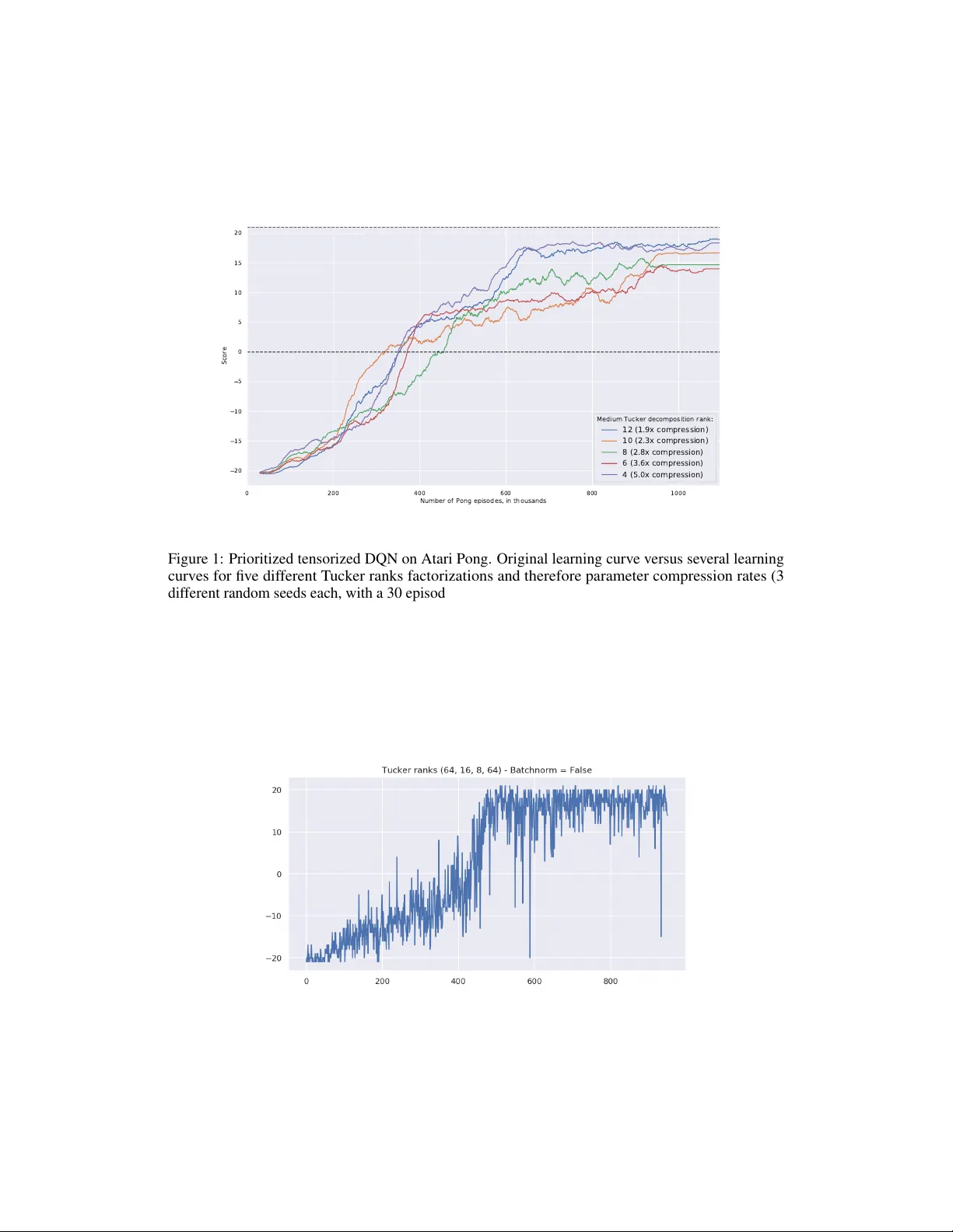
Biologically inspir ed ar chitectur es f or sample-efficient deep r einf orcement lear ning Pierre H. Richemond Imperial College London phr17@imperial.ac.uk Arinbjörn K olbeinsson Imperial College London ak711@imperial.ac.uk Y ike Guo Imperial College London y.guo@imperial.ac.uk Abstract Deep reinforcement learning requires a hea vy price in terms of sample efficienc y and ov erparameterization in the neural networks used for function approximation. In this w ork, we use tensor factorization in order to learn more compact representa- tion for reinforcement learning policies. W e show empirically that in the lo w-data regime, it is possible to learn online policies with 2 to 10 times less total coef fi- cients, with little to no loss of performance. W e also lev erage progress in second order optimization, and use the theory of wavelet scattering to further reduce the number of learned coef ficients, by foregoing learning the topmost con v olutional layer filters altogether . W e e valuate our results on the Atari suite against recent baseline algorithms that represent the state-of-the-art in data efficienc y , and get comparable results with an order of magnitude gain in weight parsimony . 1 Introduction & Related W ork The successes of deep reinforcement learning (thereafter ’RL ’) come at a heavy computational price. It is well known that achie ving human-le vel performance in domains such as Atari [ 1 , 2 , 3 ] requires hundreds of millions of frames of en vironment interaction. As such, the problem of sample efficienc y in reinforcement learning is of critical importance. Sev eral tracks of concurrent research are being in vestigated, and ha ve reduced by orders of magnitude the number of en vironment interactions required for good performance beyond the previous benchmark of biologically-inspired episodic control methods [4, 5] to a couple hours of human gameplay time [6, 7]. Ho wever , while the data-efficienc y of RL methods has seen recent drastic performance, their function approximators still use millions of learned weights, potentially still leaving them heavily overpa- rameterized. Independently motiv ated by biological facts like the beha vioural readiness of newborn animals, sev eral authors [ 8 , 9 , 10 ] hav e recently looked at doing aw ay with learning so many weights for RL tasks. Smaller networks not only train faster , but may yet of fer another av enue for gains in the form of better generalization [ 11 ]. V ery recent work from [ 8 ] studies the ef fect of inducti ve bias of neural architectures in reinforcement learning ; they fore go training altogether, b ut transfer networks that only obtain ’better than chance performance on MNIST’. In similar fashion, [ 10 ] in vestigate the ef fect of random projections in the restricted setting of imitation learning. Finally , [ 9 ] manage human-lev el performance on the Atari suite using a separate dictionary learning procedure for their features, bypassing the usual end-to-end learning paradigm. The perspecti ve of neural architecture search applied to RL appears difficult, if not computationally ine xtricable. Concurrently , the study of biologically-inspired models of learning has exhibited two mathematical characterizations that might be critical in explaining ho w biological learning takes place so ef ficiently . First, the low-rank properties of learned perceptual manifolds [ 12 , 13 ] are giving rise to a rich theory borrowing from statistical physics. Second, another well known line of work has identified Gabor filters (and more generally w avelet filter -like structures) in the actual visual cortex of animals [ 14 ], and linked those to sparsity-promoting methods and dictionary learning [ 15 , 16 , 17 ]. But these Deep Reinforcement Learning W orkshop, NeurIPS 2019, V ancouver , Canada. breakthroughs ha ve not, so far , been reflected as inducti ve priors in the shape of modifications in deep RL neural networks architectures, which remain fairly fix ed on the Atari domain. Therefore the following questions remain: how parsimonious do function approximators in rein- forcement learning need to be, in order to maintain good performance? And can we be at once sample-efficient and weight-ef ficient ? In this work, we turn to the mathematical theories of tensor factorization [ 18 ], second-order optimization [ 19 , 20 ] and wa velet scattering [ 21 ] to answer this question positiv ely and empirically , in a model-free setting. T o the best of our kno wledge, this is the first time those fields hav e been combined together in this context, and that tensor factorization is applied to deep RL. 2 Background 2.1 Deep Reinfor cement Learning W e consider the standard Marko v Decision Process frame work as in [ 1 ]). This setting is characterised by a tuple h S, A, T , R, γ i , where S is a set of states, A a set of actions, R a rew ard function that is the immediate, intrinsic desirability of a certain state, T a transition dynamics and γ ∈ [0 , 1] a discount factor . The purpose of the RL problem is to to find a policy π , which represents a mapping from states to a probability distribution over actions, that is optimal, i.e., that maximizes the expected cumulati ve discounted return P ∞ k =0 γ k R t + k +1 at each state s t ∈ S . In Q-learning, the policy is given implicitly by acting greedily or  -greedily with respect to learned action-value functions q π ( s, a ) , that are learned follo wing the Bellman equation. In deep Q-learning , q θ becomes parameterized by the weights θ of a neural network and one minimizes the e xpected Bellman loss : E  R t +1 + γ t +1 max a 0 q θ ( S t +1 , a 0 ) − q θ ( S t , A t )  2 In practice, this is implemented stochastically via uniform sampling of transitions in an experience replay buf fer , as is done in the seminal paper [ 2 ]. Several algorithmic refinements to that approach exist. First, Double Q-learning [ 22 ] proposes to decouple learning between two networks in order to alle viate the Q-v alue ov erestimation problem. Second, dueling Q-networks [ 23 ] e xplicitly decompose the learning of an action-value function q θ ( s, a ) as the sum of an action-independent state-value, much like what is traditionally done in polic y gradient methods [ 1 ], implemented via a two-headed neural network architecture. Finally , prioritized RL [ 24 ] proposes to replace the uniform sampling of transitions in the experience replay buf fer with importance sampling, by prioritizing those transitions that present the most Bellman error (those transitions that are deemed the most ’ surprising’ by the agent). [ 25 ] uses extra weights to learn the v ariance of the exploration noise in a granular fashion, while [ 26 ] proposes to learn a full distribution of action-v alues for each action and state. Combined, those methods form the basis of the Rainbow algorithm in [3]. 2.2 T ensor factorization Here we introduce notations and concepts from the tensor factorization literature. An intuition is that the two main decompositions below , CP and T ucker decompositions, can be understood as multilinear algebra analogues of SVD or eigendecomposition. CP decomposition. A tensor X ∈ R I 1 × I 2 ×···× I N , can be decomposed into a sum of R rank-1 tensors, known as the Canonical-Polyadic decomposition, where R is as the rank of the decomposition. The objectiv e is to find the vectors u (1) k , u (2) k , · · · , u ( N ) k , for k = [1 . . . R ] , as well as a vector of weights λ ∈ R R such that: X = R X k =1 λ k u (1) k ◦ u (2) k ◦ · · · ◦ u ( N ) k | {z } rank-1 components T ucker decomposition. A tensor X ∈ R I 1 × I 2 ×···× I N , can be decomposed into a lo w rank approxi- mation consisting of a core G ∈ R R 1 × R 2 ×···× R N and a set of projection factors  U (0) , · · · , U ( N − 1)  , with U ( k ) ∈ R R k , ˆ I k , k ∈ (0 , · · · , N − 1) that, when projected along the corresponding dimension of 2 the core, reconstruct the full tensor X . The tensor in its decomposed form can then be written: X = G × 1 U (1) × 2 U (2) × · · · × N U ( N ) = î G ; U (1) , · · · , U ( N ) ó T ensor regression layer . For tw o tensors X ∈ R K 1 ×···× K x × I 1 ×···× I N and Y ∈ R I 1 ×···× I N × L 1 ×···× L y , we denote by hX , Y i N ∈ R K 1 ×···× K x × L 1 ×···× L y the contraction of X by Y along their N last modes; their generalized inner product is hX , Y i N = I 1 X i 1 =1 I 2 X i 2 =1 · · · I N X i n =1 X ...,i 1 ,i 2 ,...,i n Y i 1 ,i 2 ,...,i n ,... This enables us to define a tensor r e gression layer [ 27 ] that is differentiable and learnable end-to-end by gradient descent. Let us denote by X ∈ R I 1 × I 2 ×···× I N the input activ ation tensor for a sample and y ∈ R I N the label vector . A tensor regression layer estimates the regression weight tensor W ∈ R I 1 × I 2 ×···× I N under a low-rank decomposition. In the case of a Tuck er decomposition (as per our experiments) with ranks ( R 1 , · · · , R N ) , we hav e : y = hX , W i N + b with W = G × 1 U (1) × 2 U (2) · · · × N U ( N ) as G ∈ R R 1 ×···× R N , U ( k ) ∈ R I k × R k for each k in [1 . . . N ] and U ( N ) ∈ R 1 × R N . [28, 27, 29] learn parsimonious deep learning fully-connected layers thanks to lo w-rank constraints. 2.3 W avelet scattering The wavelet scattering tr ansform was originally introduced by [ 21 ] and [ 30 ] as a non-linear e xtension to the classical wavelet filter bank decomposition [ 31 ]. Its principle is as follo ws. Denoting by x ~ y [ n ] the 2-dimensional, circular conv olution of two signals x [ n ] and y [ n ] , let us assume that we have pre-defined two wav elet filter banks av ailable ¶ ψ (1) λ 1 [ n ] © λ 1 ∈ Λ 1 ¶ ψ (2) λ 2 [ n ] © λ 2 ∈ Λ 2 , with λ 1 and λ 2 two frequency indices. These wa velet filters correspond to high frequencies, so we also giv e ourselves the data of a lo wpass filter φ J [ n ] . Finally , and by opposition to traditional linear wa velet transforms, we also assume a giv en nonlinearity ρ ( t ) . Then the scattering transform is giv en by coefficients of order 0,1, and 2, respecti vely : S 0 x [ n ] = x ~ φ J [ n ] S 1 x [ n, λ 1 ] = ρ Ä x ~ ψ (1) λ 1 ä ~ φ J [ n ] λ 1 ∈ Λ 1 S 2 x [ n, λ 1 , λ 2 ] = ρ Ä ρ Ä x ~ ψ (1) λ 1 ä ~ ψ (2) λ 2 ä ~ φ J [ n ] λ 1 ∈ Λ 1 , λ 2 ∈ Λ 2 ( λ 1 ) This can effecti vely be understood and implemented as a two-layer conv olutional neural network whose weights are not learned but rather frozen and given by the coef ficients of wavelets ψ and φ (with Gabor filters as a special case [ 31 ]). The difference with traditional filter banks comes from the iterated modulus/nonlinear activ ation function applied at each stage, much like in traditional deep learning conv olutional neural networks. In practice, the potential of scattering transforms to accelerate deep learning by providing ready-made con volutional layers weights has been in vestigated in [32, 33, 34]. 2.4 Second order optimization with K-F A C While stochastic gradient descent is usually performed purely from gradient observ ations deriv ed from auto-differentiation, f aster , second order optimization methods first multiply the weights’ θ gradient vector ∇ θ by a preconditioning matrix, yielding the weight update θ ← θ − η G − 1 ∇ θ . In the case of second order methods, the matrix G − 1 is chosen to act as a tractable iterativ e approximation to the in verse Hessian or Empirical Fisher Information Matrix [ 19 ] of the neural network model in question. Kronecker -factored approximate curv ature or K-F A C [ 20 ] enforces a Kronecker decomposition of the type G = A ⊗ B , with A and B being smaller, architecture-dependent matrices. Unlike the abov e methods, K-F A C has been applied as a plug-in in the RL literature and been shown to promote con ver gence [35]. 3 3 Methods & Experimental Results W e do take as a baseline method the data-efficient Rainbow of [ 6 ]. Howe ver , we change the architecture of the neural network function approximators used, in accordance with the principles described abov e, combining them to reflect inductiv e biases promoting fewer learnable parameters: • W e replace the fully-connected, linear layers used in the Rainbow [ 3 ] and data-efficient Rainbow [ 6 ] by tensor regression layers [ 27 ] in order to learn low-r ank policies (ranks in appendix). • W e use either the K-F A C [20] second order stochastic optimizer , or AD AM [36]. • W e combine the two methods with various rank and therefore weight compression ratios and ev aluate those on the same subset of Atari games as [6, 7]. • When possible, we replace the first conv olutional layer in the approximating neural network with a scattering layer for further gains in terms of learnable weights. For all our Atari experiments, we used OpenAI Gym [ 37 ], and a combination of PyT orch [ 38 ], T ensorL y [ 39 ] and Kymatio [ 40 ] for auto-differentiation. W e ev aluated our agents in the low-data regime of 100,000 steps, on half the games, with 3 different random seeds for reproducibility [ 41 ]. Our specific hyperparameters are described in appendix. W e report our results in tables 1 and 2. Game SimPLe Rainbow Denoised TRL 2.5x TRL 5x TRL 10x alien 405 740 684 688 454 566 amidar 88 189 154 118 86 84 assault 369 431 321 543 521 513 asterix 1090 471 500 459 554 363 bank_heist 8 51 77 59 134 42 battle_zone 5184 10125 9378 14466 13466 5744 boxing 9 0.2 1 -2 -2 -5 breakout 13 2 3 2 2 4 chopper_command 1247 862 1293 1255 1243 1106 crazy_climber 39828 16185 9977 3928 4225 2340 demon_attack 170 508 450 362 263 175 freew ay 20 28 28 26 25 24 frostbite 255 867 1101 659 912 231 gopher 771 349 391 278 255 396 hero 1295 6857 3013 5351 3732 3321 jamesbond 125 302 295 215 213 218 kangaroo 323 779 1002 804 715 400 krull 4540 2852 2656 2333 2275 2308 kung_fu_master 17257 14346 4037 9392 4764 4031 ms_pacman 763 1204 1053 818 838 517 pong 5 -19 -20 -20 -19 -21 priv ate_eye 58 98 100 51 100 1128 qbert 560 1153 672 697 581 733 road_runner 5169.4 9600 5426 6965 3914 1319 seaquest 371 354 387 345 350 287 up_n_down 2153 2877 5123 2197 2302 2179 A verage (vs. Rainbow) 100% 118% 96% 90% 71% T able 1: Mean episode returns as reported in SimPLe [ 7 ] and data-efficient Rainbo w [ 6 ], versus our agents, on 26 Atari games. ’Denoised’ is the NoisyNet ablation of Rainbow; ’TRL ’ shows the performance of the data-efficient Rainbo w with tensor regression layers substituted for linear ones. T able 1 shows proof of concept of the online learning of low-rank policies, with a loss of final performance v arying in proportion to the compression in the lo w-rank linear layers, very much like in the deep learning literature [ 28 , 27 ]. The number of coef ficients in the original data-efficient Rainbo w 4 is of the order of magnitude of 1M and v aries depending on the en vironment and its action-space size. The corresponding tensor regression layer ranks are in appendix, and chosen to tar get 400k, 200k and 100k coef ficients respectiv ely . While individual game results tend to decrease monotonously with increasing compression, we observ e that they are noisy as per the nature of e xploration in RL, and av erage scores reported correspond with the intuition that performance seems to decrease fast after a certain ov erparameterization threshold is crossed. T o take this noisy character into account, we take care to be conserv ativ e and report the av erage of the final three episodes of the learned polic y after 80000, 90000 and 100000 steps, respecti vely . Also, so as to not muddy the discussion and pro vide fair baselines, we do report on the NoisyNet [25] ablation of Rainbo w (’Denoised’ columns), as the NoisyLinear layer doubles up the number of coefficients required and actually performs worse in our experiments. Interestingly , the approximation error in tensor factorization seems to play a role akin to promoting exploration noise. W e then proceed to assess the impact of second-order optimization to our architecture by substituting AD AM optimization for K-F A C, and introducing scattering, in table 2 (only a handful results being av ailable with scattering, due to computational limitations). In spite of our conserv ati ve reporting, the efficienc y boost from using a second order scheme more than makes up for low-rank approximation error with fiv e times less coefficients than [ 6 ], suggesting that learning with a full order of magnitude less coefficients is well within reach of our techniques. Game KF A C+Denoised KF AC+TRL5x KF A C+TRL10x Scattering alien 996 734 643 441 amidar 163 101 98 84 assault 501 491 496 434 asterix 537 549 526 502 bank_heist 100 73 57 29 battle_zone 8622 15178 6156 4311 boxing 0 -4 -1 -9 breakout 3 3 2 2 chopper_command 692 611 1302 441 crazy_climber 14242 12377 3546 740 demon_attack 582 434 318 692 freew ay 26 26 24 19 frostbite 1760 718 1483 654 gopher 363 341 265 172 hero 4188 6284 4206 4127 jamesbond 263 327 217 48 kangaroo 2085 613 588 391 krull 2855 3441 3392 772 kung_fu_master 8481 10738 7357 233 ms_pacman 1137 920 867 613 pong -19.3 -19 -19 -20 priv ate_eye 56 100 100 0 qbert 731 520 538 475 road_runner 4516 8493 7224 1278 seaquest 349 317 520 213 up_n_down 2557 2291 2108 993 A verage (vs. Rainbow) 114% 109% 98% 56% T able 2: Mean episode returns of our low-rank agents with second-order optimization and scattering. 4 Conclusion W e hav e demonstrated that in the lo w-data regime, it is possible to le verage biologically plausible characterizations of experience data (namely low-rank properties and wa velet scattering separability) to exhibit architectures that learn policies with many times less weights than current baselines, in an online fashion . W e do hope that this will lead to even further progress to wards sample efficienc y and speedy exploration methods. Further work will first focus on thorough ev aluation and research of scattering architectures in order to achie ve further g ains, and second in vestigate additional, orthogonal biologically-friendly research directions such as promoting sparsity . 5 References [1] R. S. Sutton and A. G. Barto, Reinforcement Learning: An Intr oduction . The MIT Press, second ed., 2018. [2] V . Mnih, K. Kavukcuoglu, D. Silv er, A. Graves, I. Antonoglou, D. W ierstra, and M. Riedmiller, “Playing Atari with Deep Reinforcement Learning, ” arXiv e-prints , Dec. 2013. [3] M. Hessel, J. Modayil, H. van Hasselt, T . Schaul, G. Ostrovski, W . Dabney, D. Hor gan, B. Piot, M. Azar, and D. Silver, “Rainbo w: Combining Improv ements in Deep Reinforcement Learning, ” arXiv e-prints , Oct. 2017. [4] C. Blundell, B. Uria, A. Pritzel, Y . Li, A. Ruderman, J. Z. Leibo, J. Rae, D. W ierstra, and D. Hassabis, “Model-Free Episodic Control, ” arXiv e-prints , June 2016. [5] A. Pritzel, B. Uria, S. Sriniv asan, A. Puigdomènech, O. V inyals, D. Hassabis, D. W ierstra, and C. Blundell, “Neural Episodic Control, ” arXiv e-prints , Mar . 2017. [6] H. van Hasselt, M. Hessel, and J. Aslanides, “When to use parametric models in reinforcement learning?, ” arXiv e-prints , June 2019. [7] L. Kaiser, M. Babaeizadeh, P . Milos, B. Osinski, R. H. Campbell, K. Czechowski, D. Erhan, C. Finn, P . K ozakowski, S. Levine, A. Mohiuddin, R. Sepassi, G. Tuck er, and H. Michalewski, “Model-Based Reinforcement Learning for Atari, ” arXiv e-prints , Mar . 2019. [8] A. Gaier and D. Ha, “W eight Agnostic Neural Networks, ” arXiv e-prints , June 2019. [9] G. Cuccu, J. T ogelius, and P . Cudre-Mauroux, “Playing Atari with Six Neurons, ” arXiv e-prints , June 2018. [10] R. W ang, C. Ciliberto, P . Amadori, and Y . Demiris, “Random Expert Distillation: Imitation Learning via Expert Policy Support Estimation, ” arXiv e-prints , May 2019. [11] C. Zhang, S. Bengio, M. Hardt, B. Recht, and O. V inyals, “Understanding deep learning requires rethinking generalization, ” arXiv e-prints , Nov . 2016. [12] S. Chung, D. D. Lee, and H. Sompolinsky, “Classification and Geometry of General Perceptual Manifolds, ” Physical Revie w X , vol. 8, p. 031003, July 2018. [13] S. Chung, D. D. Lee, and H. Sompolinsky , “Linear readout of object manifolds., ” Physical re view . E , vol. 93 6, p. 060301, 2016. [14] J. P . Jones and L. A. Palmer , “ An ev aluation of the two-dimensional gabor filter model of simple receptiv e fields in cat striate cortex., ” Journal of neur ophysiology , vol. 58 6, pp. 1233–58, 1987. [15] B. A. Olshausen and D. J. Field, “Emergence of simple-cell receptiv e field properties by learning a sparse code for natural images, ” Nature , v ol. 381, pp. 607–609, 1996. [16] B. A. Olshausen and D. J. Field, “Sparse coding with an overcomplete basis set: A strategy employed by v1?, ” V ision Resear ch , v ol. 37, pp. 3311–3325, 1997. [17] A. Hyvärinen and P . O. Hoyer , “ A two-layer sparse coding model learns simple and complex cell receptiv e fields and topography from natural images, ” V ision Resear ch , v ol. 41, pp. 2413–2423, 2001. [18] A. Cichocki, R. Zdunek, A. H. Phan, and S. Amari, Nonnegative Matrix and T ensor F actorizations - Applications to Exploratory Multi-way Data Analysis and Blind Sour ce Separation . Wile y , 2009. [19] S. ichi Amari, “Natural gradient works efficiently in learning, ” Neural Computation , v ol. 10, pp. 251–276, 1998. [20] J. Martens and R. B. Grosse, “Optimizing neural networks with kronecker-factored approximate curvature, ” ArXiv , vol. abs/1503.05671, 2015. [21] S. Mallat, “Group In variant Scattering, ” arXiv e-prints , Jan. 2011. [22] H. v an Hasselt, A. Guez, and D. Silver, “Deep Reinforcement Learning with Double Q-learning, ” arXiv e-prints , Sept. 2015. [23] Z. W ang, T . Schaul, M. Hessel, H. v an Hasselt, M. Lanctot, and N. de Freitas, “Dueling Network Architectures for Deep Reinforcement Learning, ” arXiv e-prints , Nov . 2015. [24] T . Schaul, J. Quan, I. Antonoglou, and D. Silver, “Prioritized Experience Replay, ” arXiv e-prints , Nov . 2015. [25] M. Fortunato, M. Gheshlaghi Azar, B. Piot, J. Menick, I. Osband, A. Grav es, V . Mnih, R. Munos, D. Hassabis, O. Pietquin, C. Blundell, and S. Legg, “Noisy Networks for Exploration, ” arXiv e-prints , June 2017. [26] M. G. Bellemare, W . Dabney, and R. Munos, “A Distrib utional Perspectiv e on Reinforcement Learning, ” arXiv e-prints , July 2017. [27] J. K ossaifi, Z. C. Lipton, A. Khanna, T . Furlanello, and A. Anandkumar, “T ensor Regression Networks, ” arXiv e-prints , July 2017. 6 [28] J. K ossaifi, A. Khanna, Z. C. Lipton, T . Furlanello, and A. Anandkumar, “T ensor Contraction Layers for Parsimonious Deep Nets, ” arXiv e-prints , June 2017. [29] X. Cao and G. Rabusseau, “T ensor Regression Networks with v arious Low-Rank T ensor Approximations, ” arXiv e-prints , Dec. 2017. [30] J. Bruna and S. Mallat, “In variant Scattering Con volution Networks, ” arXiv e-prints , Mar . 2012. [31] S. Mallat, A W avelet T our of Signal Processing . Academic Press, 1998. [32] E. Oyallon, S. Mallat, and L. Sifre, “Generic Deep Networks with W avelet Scattering, ” arXiv e-prints , Dec. 2013. [33] E. Oyallon, S. Zagoruyko, G. Huang, N. K omodakis, S. Lacoste-Julien, M. Blaschko, and E. Belilovsk y, “Scattering Networks for Hybrid Representation Learning, ” arXiv e-prints , Sept. 2018. [34] T . Angles and S. Mallat, “Generative networks as in verse problems with Scattering transforms, ” arXiv e-prints , May 2018. [35] Y . W u, E. Mansimov, S. Liao, R. Grosse, and J. Ba, “Scalable trust-region method for deep reinforcement learning using Kronecker -factored approximation, ” arXiv e-prints , Aug. 2017. [36] D. P . Kingma and J. Ba, “Adam: A Method for Stochastic Optimization, ” arXiv e-prints , Dec. 2014. [37] G. Brockman, V . Cheung, L. Pettersson, J. Schneider, J. Schulman, J. T ang, and W . Zaremba, “OpenAI Gym, ” arXiv e-prints , June 2016. [38] A. Paszk e, S. Gross, S. Chintala, G. Chanan, E. Y ang, Z. DeV ito, Z. Lin, A. Desmaison, L. Antiga, and A. Lerer , “ Automatic differentiation in pytorch, ” in OpenRevie w , 2017. [39] J. K ossaifi, Y . Panagakis, A. Anandkumar, and M. P antic, “T ensorL y: T ensor Learning in Python, ” arXiv e-prints , Oct. 2016. [40] M. Andreux, T . Angles, G. Exarchakis, R. Leonarduzzi, G. Rochette, L. Thiry, J. Zarka, S. Mallat, J. andén, E. Belilovsky, J. Bruna, V . Lostanlen, M. J. Hirn, E. Oyallon, S. Zhang, C. Cella, and M. Eickenberg, “Kymatio: Scattering T ransforms in Python, ” arXiv e-prints , Dec. 2018. [41] P . Henderson, R. Islam, P . Bachman, J. Pineau, D. Precup, and D. Meger, “Deep Reinforcement Learning that Matters, ” arXiv e-prints , Sept. 2017. [42] M. Eickenberg, G. Exarchakis, M. J. Hirn, S. Mallat, and L. Thiry , “Solid harmonic wavelet scattering for predictions of molecule properties, ” The Journal of chemical physics , v ol. 148 24, p. 241732, 2018. 7 A ppendix Hyperparameters and Repr oducibility Our codebase is av ailable on request. Hyperparameters are as follows. First, our specific architecture-modified hyperparameters: Specific architecture hyperparameters V alue Scattering maximum log-scale J 3 Scattering volume width M 1 Scattering tensor input shape (1,4,84,84) Scattering tensor output shape (1,16,11,11) Scattering type Harmonic 3D, see [40, 42] Hidden linear layer rank constraint, 2.5x compression 128 Final linear layer rank constraint, 2.5x compression 48 Hidden linear layer rank constraint, 5x compression 32 Final linear layer rank constraint, 5x compression 48 Hidden linear layer rank constraint, 10x compression 16 Final linear layer rank constraint, 10x compression 10 KF AC T ikhonov re gularization parameter 0.1 KF AC Update frequenc y for in verses 100 T able 3: Our additional, architecture-specific hyperparameters. Furthermore, we mirror the Data-Efficient Rainbo w [6] baseline: Data-efficient Rainbo w hyperparameters V alue Grey-scaling T rue Observation do wn-sampling (84, 84) Frames stacked 4 Action repetitions 4 Rew ard clipping [-1, 1] T erminal on loss of life T rue Max frames per episode 108K Update Distributional Double Q T arget network update period ∗ ev ery 2000 updates Support of Q-distribution 51 bins Discount factor 0.99 Minibatch size 32 Optimizer Adam Optimizer: first moment decay 0.9 Optimizer: second moment decay 0.999 Optimizer:  0 . 00015 Max gradient norm 10 Priority exponent 0.5 Priority correction ∗∗ 0.4 → 1 Hardware NV idia 1080T i GPU Noisy nets parameter 0.1 T raining frames 400,000 Min replay size for sampling 1600 Memory size unbounded Replay period ev ery 1 steps Multi-step return length 20 Q network: channels 32, 64 Q network: filter size 5 x 5, 5 x 5 Q network: stride 5, 5 Q network: hidden units 256 Optimizer: learning rate 0.0001 T able 4: Data-efficient Rainbo w agent hyperparameters, as per [6]. 8 Standard deviations f or score runs Game Denoised TRL 2.5x TRL 10x alien 684 ± 7 688 ± 123 566 ± 38 amidar 154 ± 21 118 ± 12 84 ± 15 assault 321 ± 224 543 ± 94 513 ± 64 asterix 500 ± 124 459 ± 91 363 ± 66 bank_heist 77 ± 23 59 ± 22 42 ± 2 battle_zone 9378 ± 2042 14466 ± 2845 5744 ± 575 boxing 1 ± 2 -2 ± 1 -5 ± 1 breakout 3 ± 1.5 2 ± 1 4 ± 0.3 chopper_command 1293 ± 445 1255 ± 215 1106 ± 124 crazy_climber 9977 ± 3744 3928 ± 221 2340 ± 595 demon_attack 450 ± 49 362 ± 147 175 ± 7 freew ay 28 ± 0.6 26 ± 0 24 ± 0.5 frostbite 1101 ± 355 659 ± 523 231 ± 1 gopher 391 ± 46 278 ± 39 396 ± 24 hero 3013 ± 90 5351 ± 1948 3321 ± 598 jamesbond 295 ± 57 215 ± 42 218 ± 22 kangaroo 1002 ± 587 804 ± 289 400 ± 278 krull 2656 ± 180 2333 ± 309 2308 ± 268 kung_fu_master 4037 ± 2962 9392 ± 6289 4031 ± 3068 ms_pacman 1053 ± 193 818 ± 94 517 ± 38 pong -20 ± 0.4 -20 ± 0 -21 ± 0.1 priv ate_eye 100 ± 0 51 ± 59 1128 ± 1067 qbert 672 ± 144 697 ± 78 733 ± 291 road_runner 5426 ± 2830 6965 ± 6569 1319 ± 216 seaquest 387 ± 24 345 ± 40 287 ± 87 up_n_down 5123 ± 3146 2197 ± 231 2179 ± 178 T able 5: Standard deviations across seeds for runs presented T able 1. 9 Game KF A C+Denoised KF AC+TRL10x Scattering alien 996 ± 180 643 ± 51 441 ± 90 amidar 163 ± 15 98 ± 26 84 ± 11 assault 501 ± 85 496 ± 129 434 ± 304 asterix 537 ± 96 526 ± 64 502 ± 91 bank_heist 100 ± 14 57 ± 36 29 ± 13 battle_zone 8622 ± 5358 6156 ± 1951 4311 ± 1517 boxing 0 ± 2 -1 ± 3 -9 ± 12 breakout 3 ± 1 2 ± 2 2 ± 0 chopper_command 692 ± 81 1302 ± 328 441 ± 80 crazy_climber 14242 ± 2936 3546 ± 1231 740 ± 291 demon_attack 582 ± 130 318 ± 168 692 ± 232 freew ay 26 ± 0 24 ± 0 19 ± 1 frostbite 1760 ± 448 1483 ± 466 654 ± 709 gopher 363 ± 4 265 ± 67 172 ± 3 hero 4188 ± 1635 4206 ± 1862 4127 ± 1074 jamesbond 263 ± 22 217 ± 68 48 ± 10 kangaroo 2085 ± 2055 588 ± 5 391 ± 52 krull 2855 ± 156 3392 ± 2205 772 ± 560 kung_fu_master 8481 ± 8270 7357 ± 9200 233 ± 205 ms_pacman 1137 ± 180 867 ± 128 613 ± 159 pong -19 ± 0.6 -19 ± 1 -20 ± 0 priv ate_eye 56 ± 42 100 ± 0 0 ± 0 qbert 731 ± 256 538 ± 114 475 ± 161 road_runner 4516 ± 2869 7224 ± 4598 1278 ± 463 seaquest 349 ± 63 520 ± 97 213 ± 96 up_n_down 2557 ± 641 2108 ± 298 993 ± 244 T able 6: Standard deviations across seeds for runs presented T able 2. Further results and lear ning curves Learning curves As a simpler version of the experiments in the main text body , we show basic proof of concept on the simple P ong Atari game. Our experimental setup consists in using our o wn implementation of prioritized double DQN as a baseline, which combines algorithmic advances from [ 24 ] and [ 22 ]. W e replaced the densely connected layer of the original DQN architecture with a tensor regression layer implementing T ucker decomposition for dif ferent T ucker ranks, yielding different network compression factors. (These curves a verage three different random seeds). Qualitative beha viour . First results, both in terms of learning performance and compression factor , can be seen in figure 1. The two main findings of this experiment are that first, and o verall, the final performance of the agent remains unaffected by the tensor factorization, ev en with high compression rates nearing 10 times. Second, this obviously comes at the e xpense of stability during training - in tough compression re gimes, learning curves are slightly delayed, and their plateauing phases contain occasional noisy drawdo wns illustrating the increased difficulty of learning, as seen in figure 2. The extra pathwise noise, ho wever , can be seen as promoting exploration. 10 0 200 400 600 800 1000 Number of Pong episodes, in thousands 20 15 10 5 0 5 10 15 20 Score Medium Tucker decomposition rank: 12 (1.9x compression) 10 (2.3x compression) 8 (2.8x compression) 6 (3.6x compression) 4 (5.0x compression) Figure 1: Prioritized tensorized DQN on Atari Pong. Original learning curve versus se veral learning curves for fiv e different T ucker ranks factorizations and therefore parameter compression rates (3 dif ferent random seeds each, with a 30 episodes moving av erage for legibility). Best viewed in colour . Figure 2: Focus on a typical single run of the tensorized DQN learning. The ov erall shape of the typical learning curve is preserv ed, but drawdo wns in the plateauing phase do appear . 11