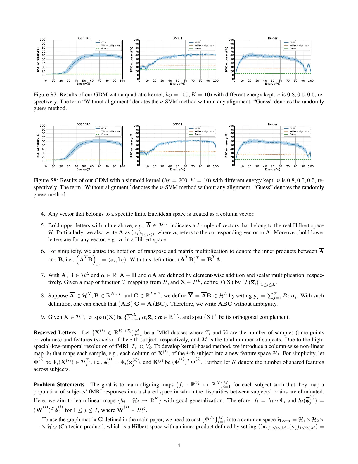
Graph-Based Decoding Model for Functional Alignment of Unaligned fMRI Data

Graph-Based Decoding Model f or Functional Alignment of Unaligned fMRI Data W eida Li, 1 Mingxia Liu, 1,2* F ang Chen, 1 Daoqiang Zhang 1* 1 College of Computer Science and T echnology & MIIT K ey Laboratory of P attern Analysis and Machine Intelligence, Nanjing Univ ersity of Aeronautics and Astronautics, Nanjing, China 2 School of Information Science and T echnology , T aishan University , T aian, China * Corresponding Authors: { mingxialiu, dqzhang } @nuaa.edu.cn Abstract Aggregating multi-subject functional magnetic resonance imaging (fMRI) data is indispensable for generating valid and general inferences from patterns distributed across human brains. The disparities in anatomical structures and functional topographies of human brains warrant aligning fMRI data across subjects. Howe ver , the existing functional alignment methods cannot handle well various kinds of fMRI datasets today , especially when they are not temporally-aligned, i.e., some of the subjects probably lack the responses to some stimuli, or different subjects might follow different sequences of stimuli. In this paper, a cross-subject graph that depicts the (dis)similarities between samples across subjects is used as a priori for dev eloping a more flexible framew ork that suits an assortment of fMRI datasets. Howe ver , the high dimen- sion of fMRI data and the use of multiple subjects makes the crude frame work time-consuming or unpractical. T o ad- dress this issue, we further regularize the frame work, so that a nov el feasible k ernel-based optimization, which permits non- linear feature extraction, could be theoretically developed. Specifically , a lo w-dimension assumption is imposed on each new feature space to av oid ov erfitting caused by the high- spatial-low-temporal resolution of fMRI data. Experimental results on five datasets suggest that the proposed method is not only superior to se veral state-of-the-art methods on temporally-aligned fMRI data, but also suitable for dealing with temporally-unaligned fMRI data. Introduction Functional Magnetic Resonance Imaging (fMRI) is an imag- ing technology used to measure neural activity by using the blood-oxygen-lev el-dependent (BOLD) contrast as an indi- cator for cogniti v e states (Logothetis 2002). The informa- tiv e patterns encoded in fMRI enable in vestig ators to study how the human brain works (Haxby , Connolly , and Guntu- palli 2014). Specifically , the use of multi-subject fMRI data is indispensable for accessing the validity and generality of the findings across subjects (T alairach and T ournoux 1988; W atson et al. 1993). From another angle, aggregating multi- subject fMRI data is also critical due to the high-spatial- low-temporal (HSL T) resolution of fMRI, i.e., the number of Copyright c  2020, Association for the Advancement of Artificial Intelligence (www .aaai.org). All rights reserved. samples (time points or volumes) is generally much smaller than the number of features (voxels) per subject. Howe ver , such aggre gation is facing a challenge that both anatomi- cal structure and functional topography v ary across subjects (Haxby et al. 2011). Hence, inter -subject alignment is an in- dispensable step in fMRI analysis. Existing studies for inter-subject alignment include anatomical alignment and functional alignment, which can work in unison. In fact, anatomical alignment is usually used as a preprocessing step for fMRI analysis, by align- ing anatomical features based on structural MRI images across subjects. T ypical examples include T alairach align- ment (T alairach and T ournoux 1988), cortical surface align- ment (Fischl et al. 1999) and so on. Ho wev er , anatom- ical alignment generated limited accuracy since the size, shape and anatomical location of functional loci dif fer across subjects (W atson et al. 1993; Rademacher et al. 1993). In contrast, functional alignment tries to directly align func- tional responses across subjects (Sabuncu et al. 2009; Con- roy et al. 2009). As more radical approaches of functional alignment, Hyperalignment (Haxby et al. 2011) and Shared Response Model (SRM) (Chen et al. 2015) learn implic- itly shared patterns across subjects, which are closely re- lated to multi-view Canonical Correlation Analysis (CCA). Though both of them hav e been extensi v ely studied and extended to an assortment, the existing related studies as- sume that the gi ven fMRI datasets should be temporally- aligned across subjects (Chen et al. 2015; T urek et al. 2018; Xu et al. 2012). In other words, the sequential fMRI time points of each subject ha ve to correspond to the same se- quence of stimuli, like all subjects watching a movie to- gether . Such a demand makes them not flexible enough as fMRI datasets today could be not temporally-aligned. For example, some subjects probably lack the responses to some stimuli, or dif ferent subjects may respond to dif fer - ent sequences of stimuli. Even though this problem could be somewhat solv ed by reordering and truncating (or down- sampling) the dataset to generate an aligned version (Chen et al. 2015), these processes may lead to an inevitable loss of information. A recent study tries to extend SRM into a semi-supervised one by exploiting labeled samples, the un- labeled samples are, howe ver , required to be temporally- aligned (T urek et al. 2017). In this paper , we aim to develop an adaptable functional alignment frame work by using a cross-subject graph that de- picts the (dis)similarities between all samples as a priori. Such a graph can be generated according to samples’ cat- egory labels or through inference (De Sa et al. 2010). From this perspecti ve, we can then focus on the (dis)similarity , which is encoded in a graph, between an y two samples rather than merely caring about if the gi ven fMRI dataset is temporally-aligned. Howe ver , the crude framework is un- practical as the related matrices are too large to be used, which is caused by the high dimension of fMRI data and the use of multiple subjects. T o address this problem, the unrefined framework is regularized so that a nov el feasible kernel-based optimization, which allows for non-linear fea- ture extraction, could be theoretically set up. W ith such a regularization, the optimal solution is, sometimes, unique. Nev ertheless, the high-spatial-low-temporal (HSL T) resolu- tion of fMRI data causes that the generated optimal solu- tion could indicate o verfitting, i.e., it aligns all aligning sam- ples perfectly . In a specific case, the culprit is that the di- mension of the subspace spanned by the aligning samples equals to the number of them. Therefore, a lo w-dimension assumption, which agrees with that the number of infor- mativ e features is generally less than the number of vox- els, is imposed on each new feature space to av oid overfit- ting. The refined framew ork, together with the proposed op- timization method, is referred to as Graph-based Decoding Model (GDM) in this paper . Notably , the objectiv e function of Hyperalignment is the same as that of our GDM (with an evident graph). The main contributions of this paper are summarized as follows: i) Unlike pre vious studies that rely on temporally-aligned data, GDM does not require temporal alignment for fMRI data. Once the prior information of the (dis)similarities among samples is a v ailable or can be inferred, one can employ our GDM to solve fMRI-based problems at hand. ii) Different from the conv entional nai ve kernel implementa- tion, the computational time of our proposed kernel-based optimization (naturally accompanied by a low-dimension assumption) is faster on the number of samples, making it suitable for processing large-scale dataset. iii) The feasible kernel-based optimization method with the low-dimension assumption is equipped with some theo- retical guarantees. In the following, we first briefly re view related works, and concisely mention the notation and problem statement. Then, the proposed method GDM will be introduced in de- tail. W e further introduce the materials used in this work, experimental setup, competing methods, and e xperimental results achie ved by different methods on both aligned and unaligned datasets, which is followed by a Conclusion sec- tion. Related proofs and additional experimental results are giv en in the Supplementary F ile . Related W orks The initial Hyperalignment (HA) method aims to seek im- plicitly shared features across subjects (Haxby et al. 2011), which is based on the orthogonal Procrustes problem. It is the first that links functional alignment and multi-view CCA. The performance of Hyperalignment on fMRI analysis is dramatically increased compared with any other anatomi- cal alignment methods. T o tackle the singularity caused by the HSL T resolution of fMRI, Regularized Hyperalignment (RHA) was de veloped by Xu et al. (Xu et al. 2012). Howe v er , neither of HA nor RHA can handle full-brain data. T o address this issue, there have been se veral works: Chen et al. de veloped a Singular V ector Decomposition Hy- peralignment (SVDHA), which firstly carries out a joint- SVD by grouping all subjects’ fMRI data for dimension re- duction across subjects (Chen et al. 2014). Later, Chen et al. introduced a Shared Response Model (SRM) which can be modeled from probabilistic perspective by assuming that each sample from the latent common space has under gone a Gaussian noise disturbance (Chen et al. 2015). Solely linear feature extra ction was considered until that Kernel Hyper- alignment (KHA) was formulated by Lorbert and Ramadge (Lorbert and Ramadge 2012). Since fMRI dataset may par- tially contain labels, a semi-supervised scheme based on SRM was studied by T urek et al. (T urek et al. 2017). On the other hand, a Searchlight approach, which takes functional alignment method as a module, was established to enhance functional alignment further by assuming that any vox el is only in connection with v oxels in its anatom- ical vicinity (Guntupalli et al. 2016). Recently , a Robust SRM that accounts for individual variations was developed by T urek et al. (T urek et al. 2018). Notation and Problem Statements Notation In this paper, the bold letters are reserved for ma- trices (upper) or vectors (lower), whereas the plain are for scalars. Gi ven any sequence of matrices { A i } M i =1 , let A ∗ be the corresponding block diagonal matrix whose diagonal matrices are { A i } M i =1 from the top left to the bottom right. Plus, for any matrix A , a i refers to its i -th column vector , A ij is its ( i, j ) -th entry , R( A ) denotes the subspace spanned by the columns of A and N( A ) is the null space of A , i.e., { x | Ax = 0 } . Moreover , any vector is treated as a column vector and the subscript of A I × J indicates its shape. Let { X i ∈ R V i × T i } M i =1 be an fMRI dataset where T i and V i are the number of samples (time points or volumes) and features (voxels) of the i -th subject, respectiv ely , and M is the total number of subjects. Due to the HSL T resolution of fMRI, T i  V i . T o dev elop a kernel-based method, we in- troduce a column-wised non-linear map Φ i that maps each sample, e.g., each column of X i , of the i -th subject into a new feature space H i , which is a Hilbert space. Unlike Ker - nel Hyperalignment (Lorbert and Ramadge 2012), subject- specific kernels are allowed. Here, dif ferent kernels could be thought to account for dif ferent structures of human brain. For simplicity , denote Φ i by setting ( φ i ) j = Φ i (( x i ) j ) for 1 ≤ j ≤ T i , and let K i be Φ T i Φ i . Plus, let K denote the number of the shared features across subjects. Assumption for Theoretical Development Generally , the dimension of H i could be infinite. For example, the re- producing kernel Hilbert space of Gaussian kernel is iso- morphic to a subspace of l 2 ( N ) (Steinwart and Christmann 2008). For clarity in the dev elopment of the optimization, we assume that H i is a finite dimensional real Hilbert space throughout the paper . The general lengthy proofs are left in the Supplementary F ile . Thus, Φ i : R V i 7→ R N i and Φ i ∈ R N i × T i where N i is the dimension of H i . The goal is to learn aligning maps { f i : R V i 7→ R K } M i =1 for each subject such that they map populations of subjects’ fMRI responses into a shared space in which the dispari- ties between subjects’ brains are eliminated. Here, we aim to learn linear aligning maps { h i : R N i 7→ R K } with good generalization. Therefore, f i = h i ◦ Φ i and h i (( φ i ) j ) = W T i ( φ i ) j for 1 ≤ j ≤ T i where W i ∈ R N i × K . Proposed Method F ormulation Cross-Subject Graph A graph about the (dis)similarities among all samples are mostly av ailable. F or example, the part of temporally-aligned samples, the category of each sample, or the distances between samples tell which samples are closely related or distinctive. T o describe such (dis)similarities, let G ∈ R T × T be a cross-subject graph matrix where T = P M i =1 T i and G ij indicates the (dis)similarity of the i -th and j -th samples, and thus G T = G . Here, i or j could refer to any sample from any subject. Objective Function Let W T be  W T 1 · · · W T M  and Y be W T Φ ∗ =  W T 1 Φ 1 · · · W T M Φ M  . Since Y ∈ R K × T contains all samples, the objectiv e function can be expressed as argmin W 1 2 T X i =1 T X j =1 G ij k y i − y j k 2 F = tr  YL Y T  (1) where L = D − G is the Laplacian matrix of the graph matrix G (Chung and Graham 1997) and D is a diagonal matrix with D ii = P T j =1 G ij . This objective function tries to separate the transformed samples y i and y j when G ij < 0 but attempts to make them close when G ij > 0 . Constraint Giv en a stimulus, suppose { z i ∈ R V i } M i =1 are subjects’ corresponding fMRI responses and the authentic aligning maps { f i : R V i 7→ R K } M i =1 are already there. Since each subject’ s fMRI responses to the same stimulus behav e like a random variable, { f i ( z i ) } M i =1 are expected to be from the same shared random variable. In other words, we do not require that f i ( z i ) = f j ( z j ) for any i, j . Therefore, the sta- tistical constraint YY T = I can be applied directly e v en if some samples are e xpected to be from the same latent response. The constraint means that each extracted shared feature is on the same scale and they are restricted be as un- correlated as possible. The crude framew ork is argmin W tr  W T Φ ∗ LΦ T ∗ W  subject to W T Φ ∗ Φ T ∗ W = I . (2) Relationship between GDM and Hyperalignment The Hyperalignment (HA) method is based on temporally- aligned dataset, assuming that T i = T 0 for i = 1 , 2 , . . . , M . Define a graph G H A by setting G ij = 1 / M when the i -th and j -th samples are aligned and G ij = 0 otherwise. Then,   W T i X i − S   2 F , which is the objective function of HA, is equal to tr  W T X ∗ ( I M T 0 × M T 0 − G H A ) X T ∗ W  since M X i =1 k W T i X i − S ∗ k 2 F = M X i =1 k W T i X i k 2 F + M k S ∗ k 2 F − 2 h M X i =1 W T i X i , S ∗ i ! =tr  W T X ∗ X T ∗ W  − tr  W T X ∗ G H A X T ∗ W  =tr  W T X ∗ ( I M T 0 × M T 0 − G H A ) X T ∗ W  . where the optimal S ∗ is 1 / M P M i =1 W T i X i . Computational Cost Problem (2) is a generalized eigen- value problem, which has been studied extensi v ely . How- ev er , with linear kernel, the size of X ∗ LX T ∗ or X ∗ X T ∗ , which is  P M i =1 V i  2 , is too tremendous to be used. For e x- ample, the dataset DS001 used in our experiment includes 16 subjects with 19174 features per subject, and then it re- quires at least 350 GB to store X ∗ LX T ∗ or X ∗ X T ∗ of shape (16 × 19174) × (16 × 19174) , which is not af fordable. Thus, an ef ficient feasible optimization is needed. The Proposition below is helpful for solving such an issue. Proposition 1 If W is one solution for problem (2), then there must be another solution that belongs to R( Φ ∗ ) , and has the same objectiv e v alue as W . Pr oof . W can be decomposed uniquely as W = W R + W N where W R ∈ R( Φ ∗ ) and W N ∈ N( Φ T ∗ ) . Since W T Φ ∗ = W T R Φ ∗ + W T N Φ ∗ = W T R Φ ∗ + 0 = W T R Φ ∗ , Plugging W R into problem (2) leads to that W R satisfies the constraint and shares the same objectiv e value with W .  Regularized Framew ork In Proposition 1, the trivial part W N exists due to the HSL T resolution of fMRI, i.e., T i  V i . Such a trifling part indicates that it does not help produce a better solution, and thus there are many optimal solutions. If the trivial part is excluded by constraint, the optimal so- lution, sometimes, become unique, and a feasible optimiza- tion will be there. More details about the uniqueness are in- cluded in the Supplementary F ile . In a nutshell, the regular- ized framew ork is expressed as argmin W tr  W T Φ ∗ LΦ T ∗ W  subject to W T Φ ∗ Φ T ∗ W = I w i ∈ R( Φ ∗ ) for 1 ≤ i ≤ K . (3) Optimization Naive Kernel-Based Optimization A simple way to solve GDM in Eq. (3) is to let W i be X i B i , where B i is a ne w variable. Then, W T X ∗ LX T ∗ W becomes B T K ∗ LK ∗ B , where B is constructed like W . The opti- mal solution of GDM can be achieved by solving a gener- alized eigen value problem. Ho wev er , with any kernel, the complexity in terms of { T i } M i =1 will be at least O ( T 3 ) where T = P M i =1 T i , meaning that it heavily depends on the num- ber of samples. In the following, we propose a more efficient kernel-based optimization algorithm. Proposed Kernel-Based Optimization Here are some tricks to solve problem (3). For each i , by spectral decom- position, K i = V i D i V T i where zero eigenv alues of K i are excluded. With U i = Φ i V i D − 1 2 i , it leads to a Singular V ec- tor Decomposition (SVD) of Φ i as Φ i = U i D 1 2 i V T i . (4) As shown in the Supplementary F ile , Φ i can be decomposed similarly when the dimension of H i is infinite. Thus, the de- velopment belo w is without loss of generality . W ith Eq. (4), Φ ∗ = U ∗ D 1 2 ∗ V T ∗ and then problem (3) is equiv alent to argmin Q tr  Q T V T ∗ L V ∗ Q  subject to Q T Q = I . (5) T o see this, denote the shape of D ∗ by S × S . Let S be { W : W T Φ ∗ Φ T ∗ W = I and w i ∈ R( Φ ∗ ) for 1 ≤ i ≤ K } and T be { Q ∈ R S × K : Q T Q = I } . Denote a map g : S 7→ T by setting g ( W ) = D 1 2 ∗ U T ∗ W . Since each column of W belongs to R( Φ ∗ ) = R( U ∗ ) , U ∗ D − 1 2 ∗ D 1 2 ∗ U T ∗ W = W , which in turn leads to that g is a bijection between S and g ( S ) = T . Plugging W = U ∗ D − 1 2 ∗ Q into problem (3) leads to problem (5). Proposition 2 Using spectral decomposition, V T ∗ L V ∗ = EΛE T where all eigen values of V T ∗ L V ∗ along the diagonal of Λ from the top left to the bottom right are in ascending order . Denote the shape of V T ∗ L V ∗ by S × S . If K ≤ S , the first K columns of E is optimal for problem (5). Pr oof . Firstly , problem (5) is equiv alent to argmin tr  R T ΛR  subject to R T R = I (6) where R = E T Q . As R T R = I infers P S i =1 P K j =1 R 2 ij = K and P K j =1 R 2 ij ≤ 1 for each i , there is tr  R T ΛR  = S X i =1 Λ ii K X j =1 R 2 ij ≥ K X i =1 Λ ii . Let R ∗ denote  I K × K 0 K × ( S − K )  T . Since tr  ( R ∗ ) T ΛR ∗  = P K i =1 Λ ii , R ∗ is optimal. There- fore, an optimal solution Q ∗ = ER ∗ for problem (5) is indeed the first K columns of E .  An Optimal Solution for Regularized Framework and Its Uniqueness Let ˆ E denote the first K columns of E and take Eq. (4) into consideration, then an optimal solution for problem (3) is W ∗ = U ∗ D − 1 2 ∗ ˆ E = Φ ∗ V ∗ D − 1 ∗ ˆ E . (7) Since each W i is separable from W , an optimal solution for subject i is W ∗ i = Φ i V i D − 1 i ˆ E i , (8) where { ˆ E i } M i =1 are block matrices of ˆ E , which is cut along the first dimension according to the dimensions of block ma- trices in D ∗ . By the equi v alences abo ve, if K > S , there is no solution satisfying the constraint in problem (3) or (6) as there is no R satisfying R T R = I . If K = S , or K < S with Λ K K < Λ ( K +1)( K +1) , the optimal solution of problem (3) is unique except being rotated. In other words, if W (1) and W (2) are two optimal solutions, there is an orthogonal matrix P such that W (1) = W (2) P . By the definition of W , it implies that the shared feature space is unique except being rotated. More details are giv en in the Supplementary F ile . Low-Dimension Assumption Potential Overfitting of GDM Suppose the dataset { X i } M i =1 is temporally-aligned, which means that T i = T j = T 0 for any i, j . Construct a graph matrix G by setting G ij = 1 if the i -th and j -th samples are temporally-aligned, and G ij = 0 otherwise. W ith this graph matrix, the objectiv e function of problem (3) with linear kernel becomes argmin W i 1 2 M X i =1 M X j =1   W T i X i − W T j X j   2 F . (9) Assume that each X i ∈ R V i × T 0 is full-column rank. Let P K × T 0 ( K ≤ T 0 ) be any matrix such that PP T = I and take Eq. (4) into consideration where Φ i is replaced by X i . W ith W ∗ i = M − 1 U i D − 1 2 i V T i P T and ( W ∗ ) T =  ( W ∗ 1 ) T · · · ( W ∗ M ) T  , W ∗ satisfies the constraints in problem (3). Howe ver , ( W ∗ i ) T Φ i = M − 1 P for each i , which implies that the generated optimal solution (8) aligns each aligning sample perfectly . The culprit is the full- column rank assumption of each X i , which is almost the case due to the HSL T resolution of fMRI, i.e., T 0  V i . Therefore, we impose a low-dimension assumption over each new feature space H i , which conforms with that the number of informative features is usually much less than the number of voxels. Suppose the low-dimension in H i is L i , then we try to fit the data in H i by an L i dimensional affine subspace 1 , i.e., argmin m i ∈ R N i F i ∈ R N i × L i T i X j =1   F i F T i (( φ i ) j − m i ) − (( φ i ) j − m i )   2 F subject to F T i F i = I . (10) 1 An L dimensional affine subspace in R N is V + c where V is an L dimensional subspace and c ∈ R N . An optimal solution is m ∗ i = T − 1 i P T i j =1 ( φ i ) j and F ∗ i be the first L i columns of U i in Eq. (4) where ( φ i ) j ← ( φ i ) j − m ∗ i for 1 ≤ j ≤ T i . The general proof for an y Hilbert space is left in the Supplementary F ile . Centralizing over Gram Matrices T o generate and ap- ply F ∗ i , it is necessary to centralize all data by the mean of the aligning data, i.e., ( φ i ) j ← ( φ i ) j − m ∗ i . Suppose Z i ∈ R V i × E i is extra fMRI data for the i -th subject. Denote all-one matrices by J . For subject i , the centralizing can be applied on the Gram matrices directly since  Φ i ( Z i ) T − T − 1 i J E i × T i Φ T i   Φ i − T − 1 i Φ i J T i × T i  = Φ i ( Z i ) T Φ i + T − 2 i J E i × T i Φ T i Φ i J T i × T i − T − 1 i J E i × T i Φ T i Φ i − T − 1 i Φ i ( Z i ) T Φ i J T i × T i . (11) From now on, suppose all Gram matrices hav e been cen- tralized. As is provided in Eq. (4), Φ i = V i D 1 2 i U T i , which is an SVD. Denote the number of the (non-zero) singular values in D i by s i . Assume the singular v alues in D 1 2 i are in descending order and the first L i ( L i ≤ s i ) singular val- ues approximately contains p i % ( p i ∈ (0 , 100] ) energy , i.e., P L i j =1 ( D i ) 1 2 j j / P s i j =1 ( D i ) 1 2 j j ≈ p i % . By this way , the low dimension L i is controlled by p i % . Therefore, the corre- sponding low-dimensional representation of Φ i ( Z i ) would be ˆ U i ˆ U T i Φ i ( Z i ) where ˆ U i is the first L i columns of U i . Generally , with only Gram matrices, there is Φ i ( Z i ) T ˆ U i ˆ U T i ˆ U i ˆ U T i Φ i = Φ i ( Z i ) T ˆ U i ˆ U T i Φ i 6 = Φ i ( Z i ) T Φ i . Nev ertheless, the equality holds with the help of ˆ V i that is defined by the first L i columns of V i Proposition 3 Φ i ( Z i ) T Φ i ˆ V i = Φ i ( Z i ) T ˆ U i ˆ U T i Φ i ˆ V i . (12) Pr oof . Since Φ i ˆ V i = U i D 1 2 i V T i ˆ V i = ˆ U i Λ i where Λ i is the upper left L i × L i submatrix of D 1 2 i , there is ˆ U i ˆ U T i Φ i ˆ V i = ˆ U i ˆ U T i ˆ U i Λ i = ˆ U i Λ i = Φ i ˆ V i .  Therefore, the proposed kernel-based optimization can easily incorporate the low-dimension assumption ov er each new feature space. It will be shown in our experiments that this is essential for getting useful results. The overall opti- mization procedure of GDM is summarized in Algorithm 1. Complexity Analysis The shape of ˆ V T ∗ L ˆ V ∗ is L × L where L = P M i =1 L i and L i is the low-dimension of the i -th subject. Suppose the Gram matrices are gi ven, and K < T i for each i , i.e., the number of the shared features is smaller than the sample size, the complexity of GDM is O (( P M i =1 T 3 i ) + L ( L 2 + T 2 + LT )) where T = P M i =1 T i . If each low-dimension L i is fix ed, Algorithm 1 Graph-Based Decoding Model (GDM) Input: Aligning data { X i ∈ R V i × T i } M i =1 , the number of the shared features K , the energy { p i % } M i =1 to be kept, a specific Laplacian matrix L and kernel functions for each subject. 1: For each i , standardize X i such that it has zero mean along the second dimension and the variance of each feature, i.e., vox el, is 1 . 2: Generate { K i } M i =1 via specified kernel functions. 3: Centralize Gram matrices: K i ← K i + T − 2 i J T i × T i K i J T i × T i − T − 1 i J T i × T i K i − T − 1 i K i J T i × T i 4: for i ← 1 to M do 5: K i = V i D i V T i by spectral decomposition. The eigen v alues in D i is in descending order . 6: Find L i such that the first L i diagonal elements of D 1 2 i contains approximately p i % energy . 7: Let ˆ V i be the first L i columns of V i . 8: Let ˆ D i be the top left L i × L i submatrix of D i . 9: end for 10: By spectral decomposition, ˆ V T ∗ L ˆ V ∗ = EΣE T where the diagonal elements of Σ is ascending. 11: Let ˆ E be the first K columns of E and then cut ˆ E along the first dimension such that ˆ E i ∈ R L i × K . 12: For 1 ≤ i ≤ M , W ∗ i ← Φ i ˆ V i ˆ D − 1 i ˆ E i . the complexity thus becomes O (( P M i =1 T 3 i ) + T 2 ) . Notably , it could be reduced into O (max 1 ≤ i ≤ M T 3 i + T 2 ) by using parallel programming. By contrast, the naive kernel scheme cannot be parallelized, and the complexity of employing it is O ( T 3 ) . Therefore, our proposed kernel method is more efficient compared to the naiv e kernel scheme. Besides, dif- ferent from methods based on iterati ve optimization algo- rithms, one can obtain the optimal solution of GDM directly . Experiments Materials W e utilize five datasets shared by openfmri.org and Chen et al. (Chen et al. 2015). The relev ant informa- tion about each dataset is outlined in T able 1. Raw datasets are preprocessed by using FSL (https://fsl.fmrib .ox.ac.uk/), following a standard process (i.e., slice timing, anatomical alignment, normalization, and smoothing). The default pa- rameters in FSL were taken when the dataset does not pro- vide. The description of each dataset is as follows: (1) DS105 : The fMRI data were measured while six sub- jects viewed gray-scale images of faces, houses, cats, bot- tles, scissors, shoes, chairs, and nonsense images (Haxby et al. 2001). Hence, there are totally 8 categories in this dataset. Here, DS105WB contains the whole-brain fMRI data while the data in DS105R OI are based on a region of interest. (2) DS011 : Fourteen subjects participated in a single task (weather prediction). In the first phase, they learned to pre- dict weather outcomes (rain or sun) for two different cities. After learning, the y predicted weather (Foerde, Knowlton, and Poldrack 2006). Thus, there are two cogniti ve states. T able 1: The brief information and parameter settings for each dataset. Here, K is the number of the shared features, energy p % is set for all subjects, ν is related to ν -SVM. Dataset #subject #sample/subject #feature #category K energy( p % ) ν #subject left out DS105WB 6 994 19174 8 10 82 0.8 1 DS105ROI 6 994 2294 8 10 82 0.8 1 DS011 14 271 19174 2 10 82 0.3 2 DS001 16 485 19174 4 10 82 0.5 4 DS232 10 1691 9947 4 10 82 0.8 2 Raider .Movie 10 2203 1000 — 20 35 — — Raider .Image 10 56 1000 7 — — 0.5 2 T able 2: The performance on temporally-aligned datasets is measured by BSC accuracy . The larger the better . Each performance is reported by av eraging accuracies ov er all folds with standard deviation. The bold denotes the best result on each dataset. Dataset(#class) ν -SVM HA KHA SVDHA SRM RSRM RHA GDM (Ours) DS105WB(8) 11 . 67 ± 1 . 80 39 . 70 ± 3 . 90 39 . 22 ± 4 . 50 30 . 48 ± 3 . 52 39 . 69 ± 3 . 95 40 . 01 ± 3 . 84 52 . 50 ± 4 . 28 60 . 68 ± 5 . 23 DS105ROI(8) 13 . 06 ± 2 . 93 48 . 05 ± 3 . 93 48 . 22 ± 3 . 34 41 . 33 ± 4 . 19 48 . 14 ± 3 . 17 48 . 51 ± 3 . 80 57 . 63 ± 5 . 55 62 . 22 ± 4 . 23 DS011(2) 51 . 80 ± 3 . 73 85 . 39 ± 3 . 52 85 . 79 ± 3 . 82 74 . 42 ± 4 . 40 85 . 47 ± 3 . 53 85 . 58 ± 3 . 89 91 . 80 ± 2 . 65 92 . 49 ± 2 . 24 DS232(4) 25 . 89 ± 2 . 46 69 . 34 ± 3 . 22 69 . 38 ± 3 . 16 56 . 77 ± 4 . 52 69 . 18 ± 3 . 27 69 . 25 ± 3 . 20 77 . 64 ± 2 . 75 82 . 47 ± 1 . 45 DS001(4) 34 . 32 ± 2 . 08 56 . 74 ± 1 . 63 57 . 10 ± 1 . 97 51 . 99 ± 1 . 87 56 . 83 ± 1 . 54 57 . 20 ± 1 . 30 57 . 87 ± 0 . 61 62 . 68 ± 1 . 53 Raider(7) 26 . 61 ± 3 . 80 60 . 48 ± 3 . 68 60 . 71 ± 3 . 23 58 . 99 ± 4 . 19 60 . 65 ± 4 . 16 62 . 38 ± 3 . 48 59 . 82 ± 4 . 10 64 . 52 ± 3 . 28 (3) DS001: Sixteen subjects were instructed to inflate a control balloon or a rew ard balloon on a screen. For a control balloon, subjects had merely one choice whereas the y could choose to pump or cash out for another case. After opting to pump, the balloon may explode or expand (Schonberg et al. 2012). Hence, there are four different cogniti v e states. (4) DS232 : T en subjects were instructed to respond to images of faces, scenes, objects and phrase-scrambled ver- sions of the scene images (Carlin and Kriegeskorte 2017). (5) Raider : As a commonly-used one, it collected data from 10 subjects participating in two experiments. Firstly , 10 subjects watched a movie Raiders of the Lost Ark (2203 TRs). The data of movie dataset does not contain any label. In the next experiment, the same 10 subjects were shown 7 classes of images (female face, male face, monke y face, dog face, house, chair and shoes) (Chen et al. 2015). It’ s worth noting that, except for Raider , all four other datasets are not temporally-aligned. T o compare GDM with other temporal-alignment-based methods, follo wing the pre- vious study in (Chen et al. 2015), these datasets (i.e., DS105, DS011, DS001, and DS232) are reordered and truncated, or downsampled, to be aligned according to their cate gories. Experimental Setup W e follow the experiment setup with a cross-v alidation strategy in previous studies (Chen et al. 2014; Haxby et al. 2011), as illustrated by Fig. S1 and Fig. S2 in the Supplementary F ile . Specifically , except for the Raider , each subject’ s data is equally divided into two parts with each category being equally split, one is for align- ment whereas the other is for training or testing a clas- sifier . Switching the roles of the two parts and leave- k - subject-out strategy are adopted for cross-v alidation. F or in- stance, if there are 16 subjects, lea ve- 4 -subject-out leads to 16 ÷ 4 × 2 = 8 folds for cross-v alidation. For Raider dataset, the movie data is taken for alignment while the im- age data is for classification. Here, the first 2 , 202 time points of movie data are used for alignment. Then it is equally di- vided into threes parts with each part ha ving 734 samples for cross-validation. Since a leave- 2 -subject-out is used in this dataset, there are a total of 10 ÷ 2 × 3 = 15 folds when using Raider . As shown in Fig. S1 in the Supplementary F ile , the e xperiment on each dataset contains two stages: 1) aligning phase, and 2) classification phase. At the first phase, one part of all subjects’ data are fed into a functional alignment method to yield the corresponding aligning maps { f i : R V i 7→ R K } M i =1 . At the classification phase, the re- maining part of data are first mapped to the shared feature space via the learned aligning maps and then used for classi- fication model construction. Note that those data used at the aligning phase will not be used at the classification phase in our experiments. Since each dataset (or part of it) used in this paper in- cludes labels, the performance of alignment is assessed by testing ho w well a trained classifier can generalize to ne w subjects, i.e., between-subject classification (BSC) accuracy (Haxby et al. 2011). Like previous studies, ν -SVM is used for classification (Chang and Lin 2011). Competing Methods The proposed GDM method is com- pared with six state-of-the-art methods in the experiments, including (1) Hyperalignment (HA) (Haxby et al. 2011), (2) Regularized Hyperalignment (RHA) (Xu et al. 2012), (3) Kernel Hyperalignment (KHA) (Lorbert and Ramadge 2012), (4) SVD-Hyperalignment (SVDHA) (Chen et al. 2014), (5) Shared Response Model (SRM) (Chen et al. 2015), and (6) Robust SRM (RSRM) (T urek et al. 2018). All methods are implemented by ourselves in Python. 0 10 20 30 40 50 60 70 80 90 Incompleteness(%) 0 10 20 30 40 50 60 70 80 90 100 BSC Accuracy(%) Raider GDM The best of others Without alignment Guess 0 10 20 30 40 50 60 70 80 90 Incompleteness(%) 0 10 20 30 40 50 60 70 80 90 100 BSC Accuracy(%) DS105WB GDM The best of others Without alignment Guess 0 10 20 30 40 50 60 70 80 90 Incompleteness(%) 0 10 20 30 40 50 60 70 80 90 100 BSC Accuracy(%) DS232 GDM The best of others Without alignment Guess Figure 1: Performance of GDM on incomplete or unaligned datasets. Here, q % incompleteness means that q % of the aligning data are randomly removed per subject. The term “Without alignment” denotes the ν -SVM method without any alignment. “The best of others” refers to the best result of six competing methods with complete data, and “Guess” denotes the randomly guess method. 0 10 20 30 40 50 60 70 80 90 100 Energy(%) 0 10 20 30 40 50 60 70 80 90 100 BSC Accuracy(%) Raider GDM Without alignment Guess 0 10 20 30 40 50 60 70 80 90 100 Energy(%) 0 10 20 30 40 50 60 70 80 90 100 BSC Accuracy(%) DS105ROI GDM Without alignment Guess 0 10 20 30 40 50 60 70 80 90 100 Energy(%) 0 10 20 30 40 50 60 70 80 90 100 BSC Accuracy(%) DS001 GDM Without alignment Guess Figure 2: The necessity of low-dimension assumption for GDM. Here, p % energy shows how much energy is nearly kept per subject. The term “W ithout alignment” denotes the ν -SVM method without any alignment. The parameter settings for each dataset are briefly listed in T able 1. F or a fair comparison, the parameter ν in ν -SVM (with a linear kernel) is fixed for all methods on each dataset. For six competing methods, we choose the optimal hyperpa- rameters according to their original papers. F or our GDM model, a linear kernel is fixed, while the influence of differ- ent kernels are shown in Figs. S3-S8 in the Supplementary F ile . For the Raider dataset, we set G ij = 1 if the i -th and j - th samples are temporally aligned; and G ij = 0 , otherwise. For the other datasets, we set G ij = 1 if the i -th and j -th samples are in the same cate gory; and G ij = − 1 , otherwise. Results on Aligned Datasets On the temporally-aligned datasets, we report the BSC accuracy v alues achie ved by eight different methods in T able 2. As can be seen from T a- ble 2, for each aligned dataset, the proposed GDM method consistently outperforms the competing methods in terms of BSC accurac y . For example, GDM achiev es the improve- ment of > 8% compared to the second best result (i.e., 52 . 50 of RHA) on the DIS105WB dataset. Results on Unaligned Datasets T o assess the perfor- mance of GDM when dealing with unaligned data, we ran- domly remove some data from each aligned dataset. Here, the term q % incompleteness means that q percent of aligning data are randomly removed per subject. The corresponding results are shown in Fig. 1. Notably , six competing meth- ods (i.e., HA, RHA, KHA, SVDHA, SRM, and RSRM) cannot be applied to such incomplete datasets since they are designed for aligned data. More results can be found in Figs. S3-S5 in the Supplementary F ile . From Fig. 1, one can observe that our GDM is able to preserve a dominant BSC accuracy with incompleteness up to at least 20% . For the DS232 dataset, the performance of GDM still beats others with 50% incompleteness. These results further validate the superiority of GDM in handling unaligned data. Necessity of Low-Dimension Assumption T o e valuate the influence of lo w-dimension assumption on GDM, we perform another group of experiments to study the BSC v al- ues achiev ed by GDM with dif ferent energy ratios kept on three datasets, with results reported in Figure 2. This fig- ure suggests that the best results are not achie ved by GDM with 100% energy on each dataset, thus v erifying the im- portance of the low-dimension assumption. Besides, on the Raider dataset, GDM still achiev es a good result with around 20% ener gy kept. W e conjecture that it results from the fact that the movie data contain much richer information than the visual data generated from simple objects. More results can be found in Figs. S6-S8 in the Supplementary F ile . Conclusion As an essential step in fMRI analysis, functional alignment remov es the differences between subjects’ brains so that multi-subject fMRI data can be aggregated to make v alid and general inferences. Ho wev er , the existing methods can- not well handle unaligned fMRI datasets. In this paper , a flexible frame work is dev eloped on a cross-subject graph that depicts the (dis)similarities among all samples. T o re- duce the computational cost, the frame work is regularized so that a novel feasible kernel-based optimization is analyt- ically dev eloped. T o a void ov erfitting caused by the HSL T resolution of fMRI, a low-dimension assumption is made ov er each new feature space, and we also propose a way to incorporate such an assumption into our proposed optimiza- tion. Experimental results attest to the superiority of GDM. In the future, we plan to study how to construct an informa- tiv e graph matrix in dif ferent situations. Acknowledgments This work was in part supported by the National Natural Science F oundation of China (Nos. 61876082, 61732006, 61861130366, 61703301), the National Ke y R&D Program of China (Nos. 2018YFC2001600, 2018YFC2001602), the T aishan Scholar Program of Shandong Province in China, and the Shandong Natural Science Foundation for Distin- guished Y oung Scholar in China (No. ZR2019YQ27). References [Carlin and Kriegeskorte 2017] Carlin, J. D., and Krie geskorte, N. 2017. Adjudicating between face-coding models with individual-f ace fMRI responses. PLoS Computational Biology 13(7):e1005604. [Chang and Lin 2011] Chang, C.-C., and Lin, C.-J. 2011. Lib- svm: a library for support v ector machines. ACM T ransactions on Intelligent Systems and T echnology 2(3):27. [Chen et al. 2014] Chen, P .-H.; Guntupalli, J. S.; Haxby , J. V .; and Ramadge, P . J. 2014. Joint svd-hyperalignment for multi-subject fMRI data alignment. In 2014 IEEE Interna- tional W orkshop on Machine Learning for Signal Pr ocessing (MLSP) , 1–6. IEEE. [Chen et al. 2015] Chen, P .-H. C.; Chen, J.; Y eshurun, Y .; Has- son, U.; Haxby , J.; and Ramadge, P . J. 2015. A reduced- dimension fMRI shared response model. In Advances in Neu- ral Information Pr ocessing Systems (NIPS) , 460–468. [Chung and Graham 1997] Chung, F . R., and Graham, F . C. 1997. Spectral graph theory . Number 92. American Mathe- matical Soc. [Conroy et al. 2009] Conroy , B.; Singer , B.; Haxby , J.; and Ra- madge, P . J. 2009. fMRI-based inter -subject cortical alignment using functional connecti vity . In Advances in Neural Informa- tion Pr ocessing Systems (NIPS) , 378–386. [De Sa et al. 2010] De Sa, V . R.; Gallagher , P . W .; Lewis, J. M.; and Malave, V . L. 2010. Multi-vie w kernel construction. Ma- chine Learning 79(1-2):47–71. [Fischl et al. 1999] Fischl, B.; Sereno, M. I.; T ootell, R. B.; and Dale, A. M. 1999. High-resolution intersubject av eraging and a coordinate system for the cortical surface. Human Brain Map- ping 8(4):272–284. [Foerde, Kno wlton, and Poldrack 2006] Foerde, K.; Knowlton, B. J.; and Poldrack, R. A. 2006. Modulation of competing memory systems by distraction. Pr oceedings of the National Academy of Sciences 103(31):11778–11783. [Guntupalli et al. 2016] Guntupalli, J. S.; Hanke, M.; Halchenko, Y . O.; Connolly , A. C.; Ramadge, P . J.; and Haxby , J. V . 2016. A model of representational spaces in human cortex. Cer ebral Cortex 26(6):2919–2934. [Haxby et al. 2001] Haxby , J. V .; Gobbini, M. I.; Furey , M. L.; Ishai, A.; Schouten, J. L.; and Pietrini, P . 2001. Distributed and ov erlapping representations of faces and objects in ventral temporal cortex. Science 293(5539):2425–2430. [Haxby et al. 2011] Haxby , J. V .; Guntupalli, J. S.; Connolly , A. C.; Halchenko, Y . O.; Conroy , B. R.; Gobbini, M. I.; Hanke, M.; and Ramadge, P . J. 2011. A common, high-dimensional model of the representational space in human ventral temporal cortex. Neur on 72(2):404–416. [Haxby , Connolly , and Guntupalli 2014] Haxby , J. V .; Con- nolly , A. C.; and Guntupalli, J. S. 2014. Decoding neural repre- sentational spaces using multiv ariate pattern analysis. Annual Revie w of Neur oscience 37:435–456. [Logothetis 2002] Logothetis, N. K. 2002. The neural basis of the blood–oxygen–lev el–dependent functional magnetic reso- nance imaging signal. Philosophical T r ansactions of the Royal Society of London B: Biological Sciences 357(1424):1003– 1037. [Lorbert and Ramadge 2012] Lorbert, A., and Ramadge, P . J. 2012. Kernel hyperalignment. In Advances in Neural Infor- mation Pr ocessing Systems (NIPS) , 1790–1798. [Rademacher et al. 1993] Rademacher, J.; Ca viness Jr , V .; Steinmetz, H.; and Galaburda, A. 1993. T opographical vari- ation of the human primary cortices: implications for neu- roimaging, brain mapping, and neurobiology . Cer ebral Cortex 3(4):313–329. [Sabuncu et al. 2009] Sabuncu, M. R.; Singer , B. D.; Con- roy , B.; Bryan, R. E.; Ramadge, P . J.; and Haxby , J. V . 2009. Function-based i ntersubject alignment of human cortical anatomy . Cer ebral Cortex 20(1):130–140. [Schonberg et al. 2012] Schonberg, T .; Fox, C. R.; Mumford, J. A.; Congdon, E.; T repel, C.; and Poldrack, R. A. 2012. Decreasing ventromedial prefrontal cortex activity during se- quential risk-taking: An fMRI in vestigation of the balloon ana- log risk task. F r ontiers in Neur oscience 6:80. [Steinwart and Christmann 2008] Steinwart, I., and Christ- mann, A. 2008. Support vector machines . Springer Science & Business Media. [T alairach and T ournoux 1988] T alairach, J., and T ournoux, P . 1988. Co-planar stereotaxic atlas of the human brain: 3- dimensional proportional system: an approach to cerebral imaging. [T urek et al. 2017] T urek, J. S.; W illke, T . L.; Chen, P .-H.; and Ramadge, P . J. 2017. A semi-supervised method for multi- subject fMRI functional alignment. In 2017 IEEE Interna- tional Conference on Acoustics, Speech and Signal Pr ocessing (ICASSP) , 1098–1102. IEEE. [T urek et al. 2018] T urek, J. S.; Ellis, C. T .; Skalaban, L. J.; T urk-Bro wne, N. B.; and Willk e, T . L. 2018. Capturing shared and individual information in fMRI data. In 2018 IEEE Inter- national Confer ence on Acoustics, Speech and Signal Process- ing (ICASSP) , 826–830. IEEE. [W atson et al. 1993] W atson, J. D.; Myers, R.; Fracko wiak, R. S.; Hajnal, J. V .; W oods, R. P .; Mazziotta, J. C.; Shipp, S.; and Zeki, S. 1993. Area v5 of the human brain: evidence from a combined study using positron emission tomography and mag- netic resonance imaging. Cerebr al Cortex 3(2):79–94. [Xu et al. 2012] Xu, H.; Lorbert, A.; Ramadge, P . J.; Guntu- palli, J. S.; and Haxby , J. V . 2012. Regularized hyperalign- ment of multi-set fMRI data. In 2012 IEEE Statistical Signal Pr ocessing W orkshop (SSP) , 229–232. IEEE. Graph-Based Decoding Model for Functional Alignment of Unaligned fMRI Data – Supplementary F ile W eida Li, Mingxia Liu, F ang Chen, Daoqiang Zhang In what follows, we will first introduce e xperimental setup used in the main text, and then present additional results achiev ed by the proposed Graph-based Decoding Model (GDM) using dif ferent kernels. Then, we present rigorous and comprehensiv e proofs for GDM and some basic proofs needed for proving GDM in an appendix section. 1 Experimental Scheme (a) Aligning Phrase Sub ject 1 Part 1 Sub ject M-k Part 1 ··· Sub ject M+k+1 Part 1 ··· Sub ject M Part 1 ! " ! #$% ! #$%& " ! # Data for Alignmen t Gene ra ting Aligni ng Maps Shar ed F eature S pace (b) Tr aining and T esting Phrase Sub ject 1 Part 2 Sub ject M-k Part 2 ··· Sub ject M- k+1 Part 2 ··· Sub ject M Part 2 Data for Classif ication Appl ing Aligni ng Maps ! " ! #$% ! #$%& " ! # Sub ject 1 Sub ject M-k Sub ject M- k+1 Sub ject M Trainin g Prediction ··· ··· Classif ier Figure S1: The paradigm of each experiment. Here, leave-k-subject-out strategy is taken. Specifically , the aligning data are nev er used in the training and testing phrase. 2 Influence of Differ ent K ernels In the main text, we empirically use a linear kernel in GDM. In the following, we study the influence of different kernels on the performance of GDM. These kernels are listed as follo ws. 1 P a r t 1 fo r Al i g n i n g Ea ch S u b j e ct ( wi t h T t i me p o i n t s ) T i me P o i nt s 𝑇 2 𝑇 2 − 1 1 2 3 P a r t 2 fo r C l a ss i fi ca ti o n 𝑇 𝑇 − 1 𝑇 2 + 1 𝑇 2 + 2 𝑇 2 + 3 … T i me Po i n t s … ( a ) T w o - fo l d t i me p o i n t p a r t i t i o n fo r e a c h s u b j e c t ( b ) Cl a s s i fi c a t i o n p h a s e : Le a ve - k - out s u b j e c t p a r t i t i o n S u b je c t 1 Pa r t 2 S u b je c t 2 Pa r t 2 S u b je c t k Pa r t 2 S u b je c t k +1 Pa r t 2 … S u b je c t M - 1 Pa r t 2 S u b je c t M Pa r t 2 S u b je c t 1 Par t 2 S ubj e c t 2 Par t 2 S u b je c t 3 Pa r t 2 S u b je c t M - k Pa r t 2 … S u b je c t M - k+ 1 Pa r t 2 S u b je c t M Pa r t 2 … 1 st F o l d k th F o l d T e s t i n g D a t a T e s t i n g D a t a T r a i n i n g D a t a T r a i n i n g D a t a … … … Figure S2: The cross-v alidation strate gy used in our e xperiments. Here, it demonstrates ho w we di vide subjects with lea v e-k- subject-out strate gy . Gaussian k ernel k ( x , y ) = e xp − k x − y k 2 hp ! , quadratic k ernel k ( x , y ) =  x T y + hp  2 , sigmoid k ernel k ( x , y ) = tanh x T y hp ! . where hp serv es as h yperparameter for each k ernel. 0 10 20 30 40 50 60 70 80 90 Incompleteness(%) 0 10 20 30 40 50 60 70 80 90 100 BSC Accuracy(%) DS105ROI GDM The best of others Without alignment Guess 0 10 20 30 40 50 60 70 80 90 Incompleteness(%) 0 10 20 30 40 50 60 70 80 90 100 BSC Accuracy(%) DS001 GDM The best of others Without alignment Guess 0 10 20 30 40 50 60 70 80 90 Incompleteness(%) 0 10 20 30 40 50 60 70 80 90 100 BSC Accuracy(%) Raider GDM The best of others Without alignment Guess Figure S3: Results of our GDM with a Gaussian k ernel ( hp = 5 , 000 , K = 10 ) with dif ferent incomplete data rates. The ener gy is 0 . 65 , 0 . 6 , 0 . 35 from left to right, ν is 0 . 8 , 0 . 5 , 0 . 5 , respecti v ely . “The best of others” refers to the best result of six competing methods with complete data. The term “W ithout alignment” denotes the ν -SVM method without an y alignment. “Guess” denotes the randomly guess method. 2.1 Additional Results on Incomplete Dataset Besides the results in Fig. 1 in the main te xt, we further report more results on incomplete or unaligned datasets, by us ing dif ferent k ernels. The e xperimental results are sho wn in Figs. S3-S5. Denote K by the number of the shared features and ν is for ν -SVM. F or each figure, q % incompleteness means that q % of the aligning data are randomly remo v ed per subject. 2 0 10 20 30 40 50 60 70 80 90 Incompleteness(%) 0 10 20 30 40 50 60 70 80 90 100 BSC Accuracy(%) DS105ROI GDM The best of others Without alignment Guess 0 10 20 30 40 50 60 70 80 90 Incompleteness(%) 0 10 20 30 40 50 60 70 80 90 100 BSC Accuracy(%) DS001 GDM The best of others Without alignment Guess 0 10 20 30 40 50 60 70 80 90 Incompleteness(%) 0 10 20 30 40 50 60 70 80 90 100 BSC Accuracy(%) Raider GDM The best of others Without alignment Guess Figure S4: Results of our GDM wi th a quadratic k ernel ( hp = 100 , K = 10 ) with dif ferent incomplete data rates. The ener gy is 0 . 8 , 0 . 7 , 0 . 35 , respecti v ely , ν is 0 . 8 , 0 . 5 , 0 . 5 , respecti v ely . “The best of others” refers to the best result of six competing methods with complete data. The term “W ithout alignment” denotes the ν -SVM method without an y alignment. “Guess” denotes the randomly guess method. 0 10 20 30 40 50 60 70 80 90 Incompleteness(%) 0 10 20 30 40 50 60 70 80 90 100 BSC Accuracy(%) DS105ROI GDM The best of others Without alignment Guess 0 10 20 30 40 50 60 70 80 90 Incompleteness(%) 0 10 20 30 40 50 60 70 80 90 100 BSC Accuracy(%) DS001 GDM The best of others Without alignment Guess 0 10 20 30 40 50 60 70 80 90 Incompleteness(%) 0 10 20 30 40 50 60 70 80 90 100 BSC Accuracy(%) Raider GDM The best of others Without alignment Guess Figure S5: Results of our GDM with a sigmoid k ernel ( hp = 200 , K = 10 ) with dif ferent incomplete data rates. The ener gy is 0 . 75 , 0 . 7 , 0 . 35 , respecti v ely , ν is 0 . 8 , 0 . 5 , 0 . 5 , respecti v ely . “The best of others” refers to the best result of six competing methods with complete data. The term “W ithout alignment” denotes the ν -SVM method without an y alignment. “Guess” denotes the randomly guess method. 2.2 Additional Results with Lo w-Dimension Assumption In the main te xt, we e v aluate the influence of lo w-dimension assumption on GDM with a linear k ernel on three datasets in Fig. 2. Here, we sho w more results of GDM with the other three types of k ernels using the lo w-dimension assumption in Figs. S6-S8. In each figure, the term p % ener gy sho ws ho w much ener gy is nearly k ept per subject. 0 10 20 30 40 50 60 70 80 90 100 Energy(%) 0 10 20 30 40 50 60 70 80 90 100 BSC Accuracy(%) DS105ROI GDM Without alignment Guess 0 10 20 30 40 50 60 70 80 90 100 Energy(%) 0 10 20 30 40 50 60 70 80 90 100 BSC Accuracy(%) DS001 GDM Without alignment Guess 0 10 20 30 40 50 60 70 80 90 100 Energy(%) 0 10 20 30 40 50 60 70 80 90 100 BSC Accuracy(%) Raider GDM Without alignment Guess Figure S6: Results of our GDM with a Gaussian k ernel ( hp = 5000 , K = 6 ) with dif ferent ener gy k ept. ν is 0 . 8 , 0 . 5 , 0 . 5 from left to right. The term “W ithout alignment” denotes the ν -SVM method without an y alignment. “Guess” denotes the randomly guess method. 3 Pr oofs f or GDM 3.1 Pr eliminaries Notation and Definitions W e focus on real Hilbert space H . 1. The bold letters are for matrices (upper) or v ectors (lo wer), while the plain are for scalars. 2. Gi v en a matrix A , a i refers to its i -th column. 3. Gi v en an y sequence of matrices { A ( i ) } M i =1 , let A ∗ denotes the corresponding block diagonal matrix whose diagonal matrices are { A ( i ) } M i =1 from the top left to the bottom right. 3 0 10 20 30 40 50 60 70 80 90 100 Energy(%) 0 10 20 30 40 50 60 70 80 90 100 BSC Accuracy(%) DS105ROI GDM Without alignment Guess 0 10 20 30 40 50 60 70 80 90 100 Energy(%) 0 10 20 30 40 50 60 70 80 90 100 BSC Accuracy(%) DS001 GDM Without alignment Guess 0 10 20 30 40 50 60 70 80 90 100 Energy(%) 0 10 20 30 40 50 60 70 80 90 100 BSC Accuracy(%) Raider GDM Without alignment Guess Figure S7: Results of our GDM with a quadratic k ernel, hp = 100 , K = 10 ) with dif ferent ener gy k ept. ν is 0 . 8 , 0 . 5 , 0 . 5 , re- specti v ely . The term “W ithout alignment” denotes the ν -SVM method without an y alignment. “Guess” denotes the randomly guess method. 0 10 20 30 40 50 60 70 80 90 100 Energy(%) 0 10 20 30 40 50 60 70 80 90 100 BSC Accuracy(%) DS105ROI GDM Without alignment Guess 0 10 20 30 40 50 60 70 80 90 100 Energy(%) 0 10 20 30 40 50 60 70 80 90 100 BSC Accuracy(%) DS001 GDM Without alignment Guess 0 10 20 30 40 50 60 70 80 90 100 Energy(%) 0 10 20 30 40 50 60 70 80 90 100 BSC Accuracy(%) Raider GDM Without alignment Guess Figure S8: Results of our GDM with a sigmoid k ernel ( hp = 200 , K = 10 ) with dif ferent ener gy k ept. ν is 0 . 8 , 0 . 5 , 0 . 5 , re- specti v ely . The term “W ithout alignment” denotes the ν -SVM method without an y alignment. “Guess” denotes the randomly guess method. 4. An y v ector that belongs to a specific finite Euclidean space is treated as a column v ector . 5. Bold upper letters with a line abo v e, e.g., A ∈ H L , indicates a L -tuple of v ectors that belong to the real Hilbert space H . P articularly , we also write A as ( a i ) 1 ≤ i ≤ L where a i refers to the corresponding v ector in A . Moreo v er , bold lo wer letters are for an y v ector , e.g., a , in a Hilbert space. 6. F or simplicity , we ab use the notation of transpose and matrix multiplication to denote the inner products between A and B , i.e.,  A T B  ij = h a i , b j i . W ith this definition, ( A T B ) T = B T A . 7. W ith A , B ∈ H L and α ∈ R , A + B and α A are defined by element-wise addition and scalar multiplication, respec- ti v ely . Gi v en a map or function T mapping from H , and X ∈ H L , define T ( X ) by ( T ( x i )) 1 ≤ i ≤ L . 8. Suppose A ∈ H N , B ∈ R N × L and C ∈ R L × P , we define Y = AB ∈ H L by setting y i = P N j =1 B j i a j . W ith such definition, one can check that  AB  C = A ( BC ) . Therefore, we write ABC without ambiguity . 9. Gi v en X ∈ H L , let span( X ) be { P L i =1 α i x i : α ∈ R L } , and span( X ) ⊥ be its orthogonal complement. Reser v ed Letters Let { X ( i ) ∈ R V i × T i } M i =1 be a fMRI dataset where T i and V i are the number of samples (time points or v olumes) and feat ures (v ox els) of the i -th subject, respecti v ely , and M is the total number of subjects. Due to the high- spacial-lo w-temporal res olution of fMRI, T i  V i . T o de v elop k ernel-based method, we introduce a column-wise non-linear map Φ i that maps each sample, e.g., each column of X ( i ) , of the i -th subject into a ne w feature space H i . F or simplicity , let Φ ( i ) be Φ i ( X ( i ) ) ∈ H T i i , i.e., φ ( i ) j = Φ i ( x ( i ) j ) , and K ( i ) be ( Φ ( i ) ) T Φ ( i ) . Further , let K denote the number of shared features across subjects. Pr oblem Statements The goal is to learn aligning maps { f i : R V i 7→ R K } M i =1 for each subject such that the y map a population of subjects’ fMRI responses into a shared space in which the disparities between subjects’ brains are eliminate d . Here, we aim to learn linear maps { h i : H i 7→ R K } with good generalization. Therefore, f i = h i ◦ Φ i and h i ( φ ( i ) j ) = ( W ( i ) ) T φ ( i ) j for 1 ≤ j ≤ T i where W ( i ) ∈ H K i . T o use the graph matrix G defined in the main paper , we need to cast { Φ ( i ) } M i =1 into a common space H com = H 1 × H 2 × · · · × H M (Cartesian product), which is a Hilbert space with an inner product defined by setting h ( x i ) 1 ≤ i ≤ M , ( y i ) 1 ≤ i ≤ M i = 4 P M i =1 h x i , y i i i where x i , y i ∈ H i and h· , ·i i is the coupled inner product of H i . F or each i , define a map C i : H i 7→ H com by setting C i ( x ) = ( y j ) 1 ≤ j ≤ M such that y j = x if j = i and 0 ∈ H j otherwise. Then, let Ψ ( i ) be C i  Φ ( i )  , after which, we group them together by letting Ψ be ( ψ (1) 1 , . . . , ψ (1) T 1 , ψ (2) 1 , . . . , ψ (2) T 2 , . . . , ψ ( M ) 1 , . . . , ψ ( M ) T M ) . Thus, Ψ ∈ H T com where T = P M i =1 T i . Moreover , define W ∈ H K com by setting w i = ( w (1) i , w (2) i , . . . , w ( M ) i ) . 3.2 The Dev elopment of GDM Since Y = W T Ψ =  ( W (1) ) T Φ (1) ( W (2) ) T Φ (2) · · · ( W ( M ) ) T Φ ( M )  contains all transformed samples across subjects, like the one in the main paper , the crude frame work can be e xpressed as argmin W tr  YL Y T  = tr  ( W T Ψ ) L ( Ψ T W )  subject to ( W T Ψ )( Ψ T W ) = I . (1) Proposition 1 If W is one solution for pr oblem (1), then ther e must be another solution that belongs to span( Ψ ) and has the same objective value as W . Pr oof. As is proved by Lemma 1, span( Ψ ) is closed. By Theorem 4.11 in [1], H com = span( Ψ ) ⊕ span( Ψ ) ⊥ , i.e., for any x ∈ H com , it can be uniquely decomposed as r ( x ) + n ( x ) where r ( x ) ∈ span( Ψ ) and n ( x ) ∈ span( Ψ ) ⊥ . Therefore, W can be unique decomposed as r ( W ) + n ( W ) . W ith W T Ψ = ( r ( W ) + n ( W )) T Ψ = r ( W ) T Ψ + n ( W ) T Ψ = r ( W ) T Ψ + 0 = r ( W ) T Ψ , r ( W ) ∈ span( Ψ ) satisfies the constraint in problem (1) and it shares the same objecti ve v alue with W .  Therefore, the framew ork can be regularized as argmin W tr  YL Y T  = tr  ( W T Ψ ) L ( Ψ T W )  subject to ( W T Ψ )( Ψ T W ) = I w i ∈ span( Ψ ) for 1 ≤ i ≤ K . (2) 3.3 The Dev elopment of Ker nel-Based Optimization For each i , by spectral decomposition, ( Φ ( i ) ) T Φ ( i ) = V ( i ) D ( i ) ( V ( i ) ) T where zero eigen v alues are excluded. W ith U ( i ) = Φ ( i ) V ( i ) ( D ( i ) ) − 1 2 and Lemma 2, it leads to an SVD of Φ ( i ) , i.e., Φ ( i ) = U ( i ) ( D ( i ) ) 1 2 ( V ( i ) ) T . (3) Like the way we construct Ψ by using { Φ ( i ) } M i =1 , we set up U by using { U ( i ) } M i =1 . Therefore, there is Ψ = UD 1 2 ∗ V T ∗ , which is an SVD of Ψ . Next, we will sho w that problem (2) is equi valent to argmin Q tr  Q T V T ∗ L V ∗ Q  subject to Q T Q = I . (4) Denote the shape of D ∗ by S × S . Let S be { W : ( W T Ψ )( Ψ T W ) = I and w i ∈ span( Ψ ) for 1 ≤ i ≤ K } and T be { Q ∈ R S × K : Q T Q = I } . Denote a map g : S 7→ T by setting g ( W ) = D 1 2 ∗  U T W  . Since w i ∈ span( Ψ ) = span( U ) for 1 ≤ i ≤ K , UD − 1 2 ∗ D 1 2 ∗  U T W  = W , which in turn leads to that g is a bijection between S and g ( S ) . Suffice to show that g ( S ) = T . Suppose Q ∈ T , let W be UD − 1 2 ∗ Q , which means w i ∈ span( Ψ ) for 1 ≤ i ≤ K . Then W T Ψ =  UD − 1 2 ∗ Q   UD 1 2 ∗ V T  = Q T D − 1 2 ∗  U T U  D 1 2 ∗ V T = Q T V T . Therefore, W ∈ S . Moreov er , g ( UD − 1 2 ∗ Q ) = D 1 2 ∗  U T  UD − 1 2 ∗ Q  = Q . As a result, the equiv alence abov e holds. 5 Proposition 2 By spectral decomposition, V T ∗ L V ∗ = EΛE T wher e all eigen values of V T ∗ L V ∗ along the diagonal of Λ fr om the top left to the bottom right ar e in ascending order . Denote the shape of V T ∗ L V ∗ by S × S . If K ≤ S , then the first K columns of E is an optimal solution for pr oblem (4). Pr oof . Firstly , problem (4) is equiv alent to argmin tr  R T ΛR  subject to R T R = I (5) where R = E T Q . Here, R T R = I implies P S i =1 P K j =1 R 2 ij = K and P K j =1 R 2 ij ≤ 1 for each i , which in turn leads to tr  R T ΛR  = S X i =1 Λ ii K X j =1 R 2 ij ≥ K X i =1 Λ ii . W ith a moment’ s thought, R ∗ =  I K × K 0 K × ( S − K )  T is exactly a global solution for problem (5). Therefore, an optimal solution Q ∗ = ER ∗ for problem (4) is indeed the first K columns of E .  Let ˆ E denote the first K columns of E , then an optimal solution for problem (2) is W ∗ = UD − 1 2 ∗ ˆ E = ΨV ∗ D − 1 ∗ ˆ E . (6) Since each W ( i ) is separable from W , an optimal solution for subject i is ( W ( i ) ) ∗ = Φ ( i ) V ( i ) ( D ( i ) ) − 1 ˆ E ( i ) where { ˆ E ( i ) } M i =1 are block matrices of ˆ E , which is cut along the first dimension according to the dimensions of block matrices in D ∗ . Proposition 3 Considering pr oblem (5), the shape of R is S × K . If K = S , or K < S with Λ K K < Λ ( K +1)( K +1) , then its optimal solution is unique except being r otated. In other wor ds, if R (1) and R 2 ar e two optimal solutions, there exists an orthogonal matrix P suc h that R (1) = R (2) P . By the equivalence between pr oblem (5) and (2), the optimal solution of pr oblem (2) has such uniqueness. Pr oof. Note that the diagonal elements along Λ are in ascending order and tr  R T ΛR  = S X i =1 Λ ii K X j =1 R 2 ij ≥ K X i =1 Λ ii . If K = S , then any orthogonal matrix has the same objecti ve v alue since tr  R T ΛR  = P S i =1 Λ ii P S j =1 R 2 ij = P S i =1 Λ ii . Suppose K < S and Λ K K < Λ ( K +1)( K +1) . For each R , we write it as R T =  S K × K T K × ( S − K )  . Suffice it to show that T = 0 if and only if R is optimal. Suppose T ij 6 = 0 , then P K i =1 P K j =1 R 2 ij < K . So, S X i =1 Λ ii K X j =1 R 2 ij = K X i =1 Λ ii K X j =1 R 2 ij + S X i = K +1 Λ ii K X j =1 R 2 ij > K X i =1 Λ ii as Λ K K < Λ ii for K + 1 ≤ i ≤ S and P S i =1 P K j =1 R 2 ij = K . If T = 0 , then P K j =1 R 2 ij = 1 for 1 ≤ i ≤ K , which means that R is optimal. Therefore, an y optimal solution ( R ∗ ) T can be expressed as  S K × K 0  . S must be orthogonal since SS T = R T R = I . By the equiv alences, any optimal solution Q ∗ of problem (4) can be written as Q ∗ = ER ∗ = ˆ ES T where ˆ E is the first K columns of E , which in turn shows that any optimal solution W ∗ can be represented by UD − 1 2 ∗ Q ∗ = ΨV ∗ D − 1 ∗ ˆ ES T . Therefore, ( W ( i ) ) ∗ = Φ ( i ) V ( i ) ( D ( i ) ) − 1 ˆ E ( i ) S T where { ˆ E ( i ) } M i =1 are block matrices of ˆ E , which is cut along the first dimension according to the dimensions of block matrices in D ∗ .  3.4 The Low-Dimension Assumption For the i -th subject, the related problem is argmin m i ∈H i , F ( i ) ∈H L i i T i X j =1    F ( i )  ( F ( i ) ) T  φ ( i ) j − m i  −  φ ( i ) j − m i     2 (7) subject to ( F ( i ) ) T F ( i ) = I . (8) 6 By Lemma 4, an optimal solution is m ∗ i = T − 1 i P T i j =1 φ ( i ) j and F ∗ i be the first L i columns of U ( i ) in Eq. (3) where φ ( i ) j ← φ ( i ) j − m ∗ i for 1 ≤ j ≤ T i . From now on, suppose all Gram matrices have been centralized. As is provided in Eq. (3), Φ ( i ) = U ( i ) ( D ( i ) ) 1 2 ( V ( i ) ) T , which is an SVD. Denote the number of (non-zero) singular values in ( D ( i ) ) 1 2 by s i . Assume that the singular values in ( D ( i ) ) 1 2 are in descending order and the first L i ( L i ≤ s i ) singular values approximately contains p i % ( p i ∈ (0 , 100] ) energy , i.e., P L i j =1 ( D ( i ) j j ) 1 2 / P s i j =1 ( D ( i ) j j ) 1 2 ≈ p i % . Let ˆ U ( i ) be the first L i vectors in U ( i ) , which is an optimal solution of problem (7), and ˆ V ( i ) be the first L i columns of V ( i ) . Suppose Z ( i ) ∈ R V i × E i is some fMRI data for subject i , and then let Z ( i ) be Φ i ( Z ( i ) ) . Note that  ˆ U ( i )  ( ˆ U ( i ) ) T Z ( i )  T  ˆ U ( i )  ( ˆ U ( i ) ) T Φ ( i )  =  ( ˆ U ( i ) ) T Z ( i )  T  ( ˆ U ( i ) ) T Φ ( i )  = ( Z ( i ) ) T  ˆ U ( i )  ( ˆ U ( i ) ) T Φ ( i )  Proposition 4  ( Z ( i ) ) T Φ ( i )  ˆ V ( i ) = ( Z ( i ) ) T  Φ ( i ) ˆ V ( i )  = ( Z ( i ) ) T  ˆ U ( i )  ( ˆ U ( i ) ) T Φ ( i )  ˆ V ( i ) . (9) Pr oof . Since Φ ( i ) ˆ V ( i ) = U ( i ) ( D ( i ) ) 1 2 ( V ( i ) ) T ˆ V ( i ) = U ( i ) ( D ( i ) ) 1 2 I L i × L i 0 ! = ˆ U ( i ) Λ ( i ) where Λ ( i ) is the upper left L i × L i submatrix of ( D ( i ) ) 1 2 , there is  ˆ U ( i )  ( ˆ U ( i ) ) T Φ ( i )  ˆ V ( i ) = ˆ U ( i )  ( ˆ U ( i ) ) T  Φ ( i ) ˆ V ( i )   = ˆ U ( i ) Λ ( i ) = Φ ( i ) ˆ V ( i ) .  4 A ppendix Lemma 1 Suppose X ∈ H N , then the subspace span( X ) = { P N i =1 α i x i : α i ∈ R } is closed. Pr oof. Without loss of generality , suppose X is linearly independent, i.e., P N i =1 α i x i = 0 = ⇒ α i = 0 . Let A be X T X ∈ R N × N . Since α T A α = h P N i =1 α i x i , P N i =1 α i x i i ≥ 0 for any α ∈ R N and A is symmetric, A is positive semi- definite. If A α = 0 , then α T A α = 0 = ⇒ P N i =1 α i x i = 0 . The linear independence of X indicates α = 0 . So, A is in vertible. By Cholesky Decomposition, A = B T B . The non-singularity of A ensures the columns of B form a basis of R N . Define a linear map T : span( X ) 7→ R N by setting T ( N X i =1 α i x i ) = N X i =1 α i b i . One can check that T is a bijection. Specifically , T is an isomorphism since h T ( y ) , T ( z ) i = h y , z i for any y , z ∈ span( X ) , which implies that T − 1 is continuous and T is an isometry . Suppose { x i } ∞ i =1 is a sequence in span( X ) such that it con ver ges to a point x ∈ H . Suffice to prove that x ∈ span( X ) . Since { x i } ∞ i =1 is a Cauchy sequence, so is { T ( x i ) } ∞ i =1 . Therefore, there exists a point c ∈ R N such that T ( x i ) → c as i → ∞ . The continuity of T − 1 shows that x i con ver ges to T − 1 ( c ) ∈ span( X ) . Since there could not be two limits in any metric space, T − 1 ( c ) = x .  Lemma 2 Suppose X ∈ H N , then it can be decomposed as X = UΣV T wher e V T V = U T U = I and Σ is a diagonal matrix in which the diagonal elements ar e all positive (and can be order ed). we refer s to such decomposition as a Singular V alue Decomposition (SVD) of X . 7 Pr oof. Firstly , remove some v ectors if need be in X to gain a list Y ∈ H M ( M ≤ N ) such that Y is linearly independent and span( X ) = span( Y ) . By Lemma 1, there is a bijection T between span( Y ) and R M . By spectral decomposition, X T X = T ( X ) T T ( X ) = VD V T where the zero eigenv alues are excluded. W e can order the diagonal elements along D if necessary . With U = T ( X ) VD − 1 2 , it leads to an SVD decomposition of T ( X ) , i.e., T ( X ) = UD 1 2 V T . Therefore, there is X = T − 1 ( UD 1 2 V T ) = T − 1 ( U ) D 1 2 V T , resulting from the fact that T − 1 is a linear map. Let U be T − 1 ( U ) and Σ be D 1 2 . The isomorphism T guarantees that U T U = I . Particularly , U = T − 1 ( U ) = T − 1  T ( X ) VD − 1 2  = XVD − 1 2 .  Lemma 3 Suppose X ∈ H N , the unique optimal solution to the pr oblem argmin m ∈H N X i =1 k x i − m k 2 is m ∗ = 1 N P N i =1 x i . Pr oof. Firstly , remove some vectors if need be in X to gain a list Y ∈ H M ( M ≤ N ) such that Y is linearly independent and span( X ) = span( Y ) . By Lemma 1, there is a bijection T between span( X ) and R M . By theorem 4.11 in [1], there exist two linear maps r and n from H into H such that r ( x ) ∈ span( X ) and n ( x ) ∈ span( X ) ⊥ for an y x ∈ H , as k x k 2 = k r ( x ) k 2 + k n ( x ) k 2 and x = r ( x ) + n ( x ) . Since k x i − m k 2 = k x i − r ( m ) k 2 + k n ( m ) k 2 ≥ k x i − r ( m ) k 2 , an optimal solution must belong to span( X ) . W ith the isomorphism T between span( X ) and R M , there is such equiv alence argmin m ∈ span( X ) N X i =1 k x i − m k 2 ⇐ ⇒ argmin m ∈ R M N X i =1 k x i − m k 2 where T ( x i ) = x i and T ( m ) = m . Considering the right-side problem, since it is con ve x and differentiable, an optimal solution m ∗ must satisfies ∂ ∂ m N X i =1 k x i − m k 2     m = m ∗ = − 2 N X i =1 ( x i − m ∗ ) = 0 , which leads to m ∗ = 1 N P N i =1 x i . Therefore, m ∗ = T − 1 ( m ∗ ) = 1 N P N i =1 x i as T − 1 is linear .  Lemma 4 Suppose X ∈ H N , let Y be ( x 1 − a , . . . , x N − a ) wher e a = 1 N P N i =1 x i . By Lemma 2, Y can be decomposed as UΣV T , i.e., Singular V alue Decomposition, wher e the diagonal elements along Σ ar e in descending order and be all positive. Denote the shape of Σ by M × M . Let R ∈ H K ar e a variable such that K ≤ M . Considering the following optimization pr oblem argmin m ∈H , R ∈H K N X i =1    R ( R T ( x i − m )) − ( x i − m )    2 subject to R T R = I , let R ∗ and m ∗ be the fir st K vectors in U and 1 N P N i =1 x i , r espectively , then ( R ∗ , m ∗ ) is an optimal solution for the problem above. 8 Pr oof. The proof is composed of two parts: 1) Firstly , we show that m ∗ is alw ays an optimal solution whatev er R is fixed. 2) Then, we prov e that R ∗ is an optimal solution when m is fixed as m ∗ . 1) m ∗ is always optimal independent of R . By Lemma 1, span( R ) is closed. By theorem 4.11 in [1], there exist two linear maps r and n from H into H such that r ( x ) ∈ span( R ) and n ( x ) ∈ span( R ) ⊥ for any x ∈ H , as k x k 2 = k r ( x ) k 2 + k n ( x ) k 2 and x = r ( x ) + n ( x ) . Therefore, N X i =1    R ( R T ( x i − m )) − ( x i − m )    2 = N X i =1     R  R T x i  − x i  −  R  R T m  − m     2 = N X i =1 k ( r ( x i ) − x i ) − ( r ( m ) − m ) k 2 = N X i =1 k n ( x i ) − n ( m ) k 2 By Lemma 3, P N i =1 k n ( x i ) − n ( m ) k 2 ≥ P N i =1    n ( x i ) − 1 N P N j =1 n ( x i )    2 for any m . Then m ∗ must be an optimal solution since n ( m ∗ ) = 1 N P N j =1 n ( x i ) whatev er n is. 2) The optimal solution of R when m is fixed as m ∗ . There is    R  R T y i  − y i    2 = h R  R T y i  , R  R T y i  i + k y i k 2 − 2 h R  R T y i  , y i i . Since R T R = I , h R  R T y i  , R  R T y i  i = h R T y i , R T y i i . By Theorem 4.22 in [1], R can be extended into a basis of H , by which it is ob vious that h R  R T y i  , y i i = h R T y i , R T y i i . Therefore, the problem we are solving is equi v alent to argmax R ∈H K N X i =1 h R T y i , R T y i i = tr  R T Y   Y T R  subject to R T R = I . By Lemma 2 , Y = UΣV T , i.e., Singular V alue Decomposition, where the singular values along Σ are in descending order and are all positiv e. Thus, R T Y = R T  UΣV T  =  R T U  ΣV T , which leads to L ( R ) = tr  R T Y   Y T R  = tr  R T U  Σ 2  U T R  . Let A be R T U ∈ R K × M . Both R T R = I K × K and U T U = I M × M provide that M X i =1 A 2 j i ≤ 1 for an y j and K X j =1 M X i =1 A 2 j i ≤ K . W ith these inequalities, there is tr  AΣ 2 A T  = M X i =1 Σ 2 ii K X j =1 A 2 j i ≤ K X i =1 Σ 2 ii . W ith a moment’ s thought, L ( R ∗ ) = P K i =1 Σ 2 ii , which confirms that R ∗ is an optimal solution.  Refer ences [1] W alter Rudin. Real and complex analysis . T ata McGraw-hill education, 2006. 9