Data-efficient Co-Adaptation of Morphology and Behaviour with Deep Reinforcement Learning

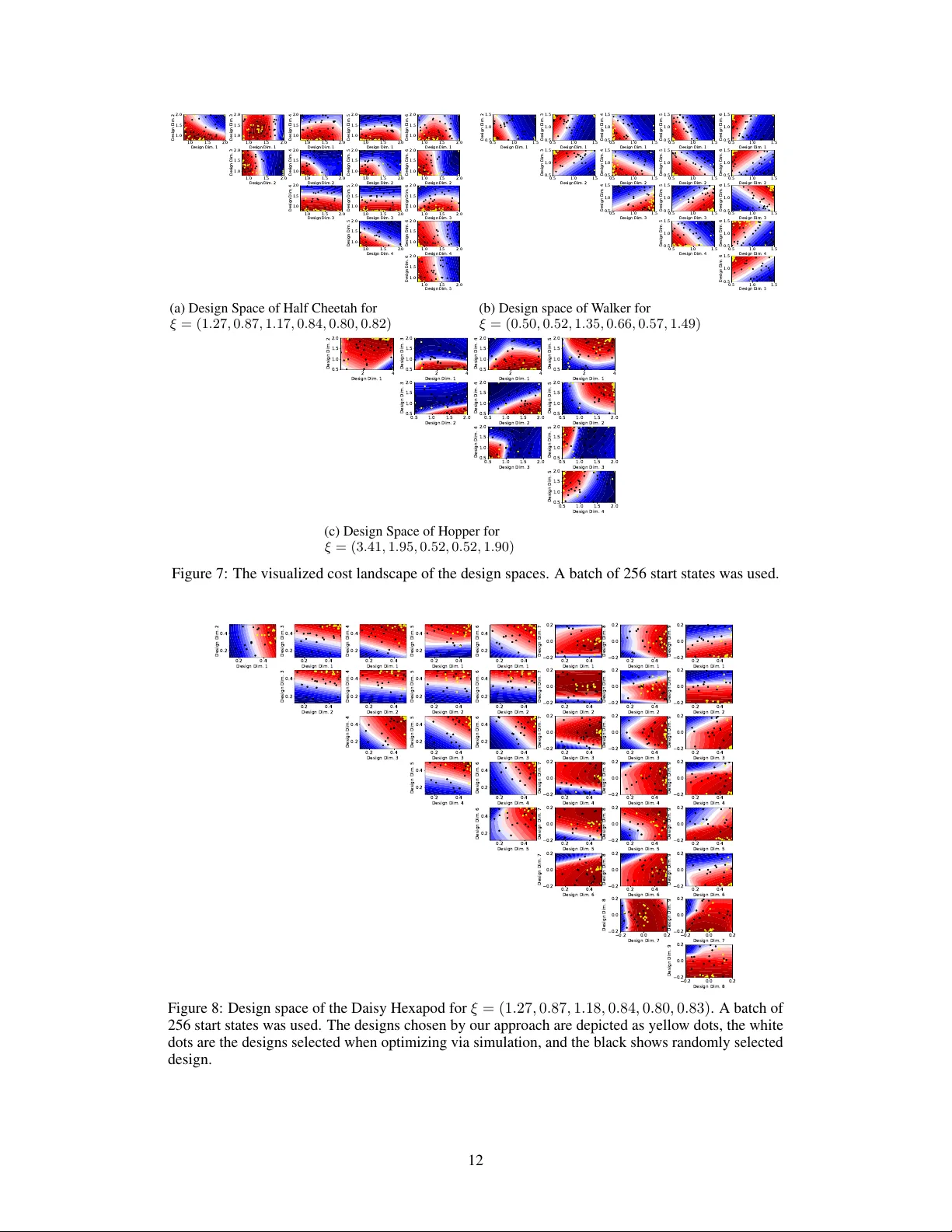
Data-efficient Co-Adaptation of Morphology and Beha viour with Deep Reinf or cement Learning Ke vin Sebastian Luck Interactiv e Robotics Lab Arizona State Univ ersity United States ksluck@asu.edu Heni Ben Amor Interactiv e Robotics Lab Arizona State Univ ersity United States hbenamor@asu.edu Roberto Calandra Facebook AI Research United States rcalandra@fb.com Abstract: Humans and animals are capable of quickly learning new beha viours to solve ne w tasks. Y et, we often forget that the y also rely on a highly specialized morphology that co-adapted with motor control throughout thousands of years. Although compelling, the idea of co-adapting morphology and beha viours in robots is often unfeasible because of the long manufacturing times, and the need to re- design an appropriate controller for each morphology . In this paper , we propose a nov el approach to automatically and ef ficiently co-adapt a robot morphology and its controller . Our approach is based on recent advances in deep reinforcement learning, and specifically the soft actor critic algorithm. Ke y to our approach is the possibility of lev eraging previously tested morphologies and behaviors to estimate the performance of new candidate morphologies. As such, we can make full use of the information a vailable for making more informed decisions, with the ultimate goal of achieving a more data-ef ficient co-adaptation (i.e., reducing the number of morphologies and beha viors tested). Simulated e xperiments sho w that our approach requires drastically less design prototypes to find good morphology-behaviour combinations, making this method particularly suitable for future co-adaptation of robot designs in the real world. Keyw ords: Co-adaptation, Morphology , Deep Reinforcement Learning 1 Introduction In nature, both morphology and behaviour of a species crucially shape its ph ysical interactions with the en vironment [ 1 ]. For e xample, the di versity in animal locomotion styles is an immediate result of the interplay between different body structures, e.g., dif ferent numbers, compositions and shapes of limbs, as well as as different neuromuscular controls, e.g., dif ferent sensory-motor loops and neural periodic patterns. Adaptation of a species to new ecological opportunities often comes with changes to both body shape and control signals – morphology and behaviour ar e co-adapted . Building upon this insight, we in vestigate in this paper a methodology for co-adaptation of the morphology and behaviour for computational agents using deep reinforcement learning. W ithout loss of generality , we focus in particular on legged locomotion. The goal of legged robots in such locomotion tasks is to transform as much electric energy as possible into directional movement [ 2 , 3 , 4 , 5 ]. T o this end, two approaches exist: 1) optimization of the behavioural policy , and 2) optimization of the robot design, which af fects the achiev able locomotion efficienc y [ 2 , 6 , 7 , 8 ]. Policy optimization is, especially in nov el or changing en vironments, often performed using reinforcement learning [ 8 , 9 ]. Design optimization is frequently based on e volutionary algorithms or e volution-inspired and use a population of design prototypes for this process (Fig. 1a ) [ 2 , 6 , 10 ]. Howev er , manufacturing and ev aluating a lar ge quantity of design candidates is often infeasible in the real w orld due to cost and time constraints, especially for larger robots. Therefore, the ev aluation of designs is often restricted to simulation, which is feasible b ut suffers from the simulation-to-reality-gap [ 11 , 12 ]. Designs and control policies optimized in simulation are often not the best possible choice for the real world, especially if the robotics system is complex and the en vironmental parameters hard to model. For example, in the work of Lipson and Pollack [ 13 ] designs were first optimized in simulation in an ev olutionary manner and then manufactured in the real world. Ho wev er , the performances of the 3rd Conference on Robot Learning (CoRL 2019), Osaka, Japan. 1 Design P r ototype 2 Design P r ototype n Design P r ototype ... Design Optimization Design P r ototype R e i n f o r c e m e n t L e a r n i n g ... (a) T raditional approach in which designs are e valuated in simulation during the design optimization process. Design Optimization Design P r ototype R einfor cement L ear ning (b) Proposed method which ev aluates designs with the learned Q- and policy network and thus reduces the amount of simulations or physical prototypes required during the design optimization process. Origi nal Design Design 6 Design 8 Design 10 Design 12 Design 14 Design 18 Design 16 Design 22 Design 24 Design 26 Design 28 Design 30 Design 32 Design 20 Design 34 Design 38 Design 40 Design 42 Design 44 Design 46 Design 48 Design 36 Design 50 (c) Designs ξ Opt selected by the proposed method for the Half-Cheetah task. Figure 1: W e propose to (b) use an actor and critic for design exploration instead of (a) creating design prototypes and ev aluating their performance in simulation or the real world. Our goal is to reduce the amount of time needed to (c) ev olve a robotic prototype in the real w orld. manufactured designs in the real world were significant lo wer than in simulation in all b ut one case (see T able 1 in [ 13 ]), e ven though ef forts were undertaken to close the simulation-to-reality gap for the described robot. The method proposed in this work caters towards the need of roboticists for data-efficienc y in respect to the number of prototypes required to achiev e an optimal design. W e are combining design optimization and reinforcement learning in such a way that the reinforcement learning process provides us with an objecti ve function for the design optimization process (Fig. 1b ). Thus, eliminating the need for a population of prototypes and requiring only one functioning prototype at a time. 2 Related W ork The work of Schaf f et al. [ 7 ] is a relati vely recent approach to combine reinforcement learning and design optimization into one framew ork. The common idea is to consider the design parameter ξ as an additional input to the policy π ( s , ξ ) and to optimize the expected re ward E [ R ] giv en the policy and design. The policy is trained such that it is able to generalize ov er many designs and is iterativ ely updated with experience collected from a population of n prototypes. The algorithm maintains a distribution over designs, whose parameters are optimized to maximize the expected rew ard. Ho wev er , this approach [ 7 ] requires the maintenance of a population of designs, which is updated ev ery t timesteps and relies on the simulator to compute the fitness of designs. Similarly , the work of David Ha [ 14 ] uses the design parameters ξ as input to the policy π ( s , ξ ) but uses REINFORCE [ 15 ] to update the design parameters. Again, this approach requires a population of design prototypes to compute the introduced population-based policy gradient for the design as well as re wards collected from the simulator . The recent method introduced by Liao et al. [ 16 ] employs Batch Bayesian Optimization to improve morphology and policies. The expected performance of designs is here learned and inferred by Gaussian Processes (GP), a second GP is also used to optimize the parameters of central pattern generators representing mov ement policies. The paper demonstrates the design optimization of a simulated micro-robot with three parameters defining the morphology . While the presented results are using a prototype population of 5 designs, the authors mention that the proposed method can handle a single prototype as well. One drawback of [ 16 ] is, ho wev er, that the GP predicting the fitness of designs is trained only with a single value per design: the single highest 2 rew ard achiev ed for a design. Since the maximum reward is potentially af fected by the initial state a robot is in, this approach has a reduced applicability to tasks with noisy or random start states. In [ 2 ], the leg lengths and controller of a quadruped robot were optimized in the real w orld. The controller was here based on the in verse kinematics of the robot and defined by tuning eight parameters. All leg se gment lengths were described by a two-dimensional design vector . T wo different e volutionary algorithms were used to optimize these parameters ov er eight generations with a population size of eight and based on the reward recei ved. While this experiment is an impressive demonstration of the potential of adapting beha viour and morphology in the real w orld, the task was simplified through the use of a re-configurable robot which is able to adapt its leg-lengths automatically . This decreases the setup-time required between experiments because manufacturing of leg-se gments or other body parts are not necessary . All four of these approaches rely on a population of design prototypes whose performance must be ev aluated in simulation or the real world, or rely on a single rew ard. 3 Problem Statement W e formalize the problem of co-adapting morphology and behavior as the optimization θ ∗ = arg max θ R | θ , (1) of the re ward R w .r .t. the variables θ = [ ξ , π ] were ξ are the morphological properties of the agent, and π the behavior . There are multiple ways to tackle this problem. One commonly used way is to decompose it as bi-le vel optimization, where we iterati vely optimize the morphology first ξ , and after fixing it, we optimize the behavior π . One adv antage of this formulation is that by decoupling the two optimization, we can take into consideration the f act that ev aluating different morphologies has an associated cost (e.g., manufacturing a physical robot) which can be substantially higher than e valuating dif ferent behaviors (e.g., running multiple controllers). In this paper , we frame the learning of the behaviors as an extension of the standard Markov decision process (MDP) [ 17 ] gi ven the additional design v ariable ξ (i.e., the context). In this model, the transition probability to reach a state s t +1 after performing action a t is giv en by p ( s t +1 | s t , a t , ξ ) and depends on design properties ξ of the agent. The reward function r ( s , a , ξ ) can be dependent on the design as well. For notational clarity , we will generally use r ( s ) in the remainder of the paper . The actions are generated from the policy π ( s , ξ ) and the goal is to maximize the expected future re ward gi ven by E π " ∞ X i =0 γ i r ( s t + i +1 , a t + i +1 , ξ )      s t = s , a i = π ( s i ) , ξ # , (2) with γ ∈ [0 , 1] being a discount factor and future states s t + i +1 produced by the transition function. Our goal is hence to maximize this objecti ve function for both the polic y π and the design ξ using deep reinforcement learning. 4 Optimization of Morphology and Beha viour W e now introduce our proposed frame work for sample-efficient optimization of beha viour and design for robotic prototypes. W e first describe our novel objecti ve function based on an actor and critic to remov e the dependency on prototypes and simulations during design optimization. Thereafter , a method is described for fast behaviour adaptation by training a copy of actor and critic primarily on experience collected with the current design prototype. W e continue with an explanation of two different design exploration mechanisms, random selection and no velty search. The chapter closes with a description of the reinforcement learning algorithms and optimization routines used. 4.1 Using the Q-Function for Design Optimization Optimizing the behaviour of an agent usually requires learning a value or Q-value function and a policy π by the means of reinforcement learning. The rationale of our approach is to extend this methodology to the ev aluation of the space of designs, thereby reducing the need for large numbers of simulations or manufactured robot prototypes. The goal of design optimization is to increase the efficienc y of the agent giv en an optimal policy for each design. The objective function for this case can be the sum of re wards collected by e valuating 3 the behaviour of the agent with this design, gi ven by max ξ E π " T X i =0 r t # , (3) where the rew ards are collected through the ex ecution of a policy π on the agent with design ξ in the real world or in simulation. T o alle viate the aforementioned problems with the e valuation through executions in simulation or real world, we instead propose to reuse the Q-function learned by a deep reinforcement learning algorithm and re-formulate our objectiv e as max ξ E π [ Q ( s , a , ξ ) | a = π ( s , ξ )] , (4) where the action a is gi ven by the policy π ( s , ξ ) . This creates a strong coupling between the design optimization and reinforcement learning loop: W e ef fectiv ely reduce the problem of finding optimal designs to the problem of training a critic which is able to generate an estimated performance of a design gi ven state and action. This means, while optimizing a policy for a design, we also train the objecti ve function gi ven abov e at the same time. W e hypothesize that, during the training process, the critic learns to distinguish and interpolate between designs due to the influence of the design on the rew ard of transitions. W e further reformulate Eq. 4 to optimize over the distribution of start states encountered in trajectories ( s 0 , a 0 , s 1 , · · · , s T ) . The objective function becomes then the expected future reward gi ven a design choice ξ . This could be, for example, the case if the leg lengths of a robot are optimized and the initial position is a standing one. Here, the initial height of the robot would v ary with the design choice. Thus, we reformulate the objectiv e function in Eq. 4 such that we optimize ov er the distribution of start states with max ξ E s 0 ∼ p ( s 0 | ξ ) [ E π [ Q ( s 0 , a 0 , ξ ) | a 0 = π ( s 0 , ξ )]] . (5) The moti vation to optimize this function over the distribution of start states is to take potential randomness in the initial positions, or e ven inaccuracies when resetting the initial position of a robot, into account. Since the distribution of start states might be unknown or e ven depend on the design, we approximate the expectation by drawing a random batch of start states s 0 from a replay buffer , which contains exclusi vely all start states seen so far . If we use a deterministic deep neural network for policy π , Eq. 5 reduces to max ξ 1 n X s ∈ s batch Q ( s , π ( s , ξ ) , ξ ) , (6) with s batch = ( s 1 0 , s 2 0 , · · · , s n 0 ) containing n randomly chosen start states. This objecti ve function can be optimized with classical global optimization methods such as Particle Sw arm Optimization (PSO) [ 18 , 19 ] or Cov ariance Matrix Adaptation - Evolution Strate gy (CMA-ES) [ 20 ]. 4.2 Design Generalization and Specialization of Actor and Critic A naiv e solution to input the design variable into the actor and critic network would be to append the design vector to the state and train a single set of networks using the experience of all designs. A more promising approach is to hav e two sets of networks: One population (pop.) actor and critic network which is trained on the training e xperience from all designs, and individual (ind.) networks which are initialized with the population network but use primarily training experience from the current design (the individual). In practice, we found it helpful to allocate 10% of the training batch for samples from the population replay buffer when training the individual networks. Essentially , this approach allows the individual networks Q Ind. and π Ind. to specialize in a fast manner to the current design and its nuances to quickly achieve maximum performance. In parallel, we are training the population networks Q Pop. and π Pop. with experience from all designs seen so far by selecting samples from the population replay b uffer Replay Pop. . These population networks are then able to better generalize across different designs and provide initial weights for the individual networks. Hence, policies do not ha ve to be learned from scratch for each new prototype. Instead, previously collected training data is used so that different designs can inform each other and make ef ficient use of all the experiences collected thus far . 4 Algorithm 1 Fast Ev olution through Actor-Critic Reinforcement Learning Initialize replay buf fers: Replay Pop. , Replay Ind. and Replay s 0 Initialize first design ξ for i ∈ (1 , 2 , · · · , M ) do π Ind. = π Pop. Q Ind. = Q Pop. Initialize and empty Replay Ind. while not finished optimizing local policy do Collect training experience ( s 0 , a 0 , r 1 , s 1 , · · · , s T , r T ) for current design ξ with policy network π Ind. Add quadruples ( s i , a i , r i +1 , s i +1 ) to Replay Ind. Add quintuples ( s i , a i , r i +1 , s i +1 , ξ ) to Replay Pop. Add start state s 0 to Replay s 0 Train netw orks π Ind. and Q Ind. with random batches from Replay Ind. Train netw orks π Pop. and Q Pop. with random batches from Replay Pop. end while if i is even then Sample batch of start states s batch = ( s 1 0 , s 2 0 , · · · , s n 0 ) from Replay s 0 Exploitation : Compute optimal design ξ with objecti ve function max ξ 1 n P s ∈ s batch Q Pop. ( s , π Pop. ( s , ξ ) , ξ ) else Exploration : Sample design ξ with exploration strategy end if end for 4.3 Exploration and Exploitation of Designs W e alternate between design e xploration and exploitation to increase the di versity of explored designs, improv e generalization capabilities of the critic and avoid an early con vergence to regions of the design space. Therefore, e very time we find an optimal design during the design optimization process with the objectiv e function (Eq. 6 ) and conclude the subsequent reinforcement learning process, we next choose one design using the exploration strategy . T o this end, we implemented two different approaches: sampling ne w designs 1) randomly , and 2) using Nov elty search [ 21 ]. W e found that using random sampling as exploration strate gy outperformed novelty search (see appendix). 4.4 Fast Ev olution through Actor -Critic Reinforcement Lear ning The proposed algorithm, Fast Ev olution through Actor-Critic Reinforcement Learning, is presented in Algorithm 1 . W e will now discuss the specifics of the used reinforcement learning algorithm and global optimization method. Ho wev er , it is worth noting that our methodology is agnostic to the specific algorithms used for design and behaviour optimization. Reinfor cement Learning Algorithm While in principal every reinforcement learning method can be employed to train the Q and policy functions necessary to optimize the designs, we use a deep reinforcement learning method due to the continuous state and action domains of our tasks. Specifi- cally , we employed the Soft-Actor-Critic (SA C) algorithm [ 22 ], a state-of-the-art deep reinforcement learning method based on the actor -critic architecture. All neural networks had three hidden layers with a layer size of 200. Per episode we train the individual networks π Ind. and Q Ind. 1000 times while the population networks π Pop. and Q Pop. are trained 250 times. The motiv ation was to assign more processing power to the individual networks to adapt quickly to a design and specialize. A batch size of 256 was used for each training updated. Optimization Algorithm T o optimize the objective function giv en in Eq. ( 6 ) , we used the global optimization method Particle Swarm Optimization (PSO) [ 18 , 19 ]. W e chose PSO primarily because of its ability to search the design space exhaustiv ely using a large number of particles. The objecti ve function (Eq. ( 6 ) ) was optimized using about 700 particles, each representing a candidate design, and updated ov er 250 iterations. Accordingly , PSO used a total contingent of 175,000 objectiv e function ev aluations to find an optimal design. T o optimize the design using rollouts in simulation, we had to reduce this number to about 1,050 design candidates, i.e. 35 particles updated o ver 30 iterations. Although this contingent is only about 0 . 6% of the size of the Q-function contingent, it takes about two times longer to ev aluate this number of designs in simulation. For e xample, on a system with an Intel Xeon CPU E5-2630 v4 CPU equipped with an NVIDIA Quadro P6000, the design optimization via simulation takes approximately 30 minutes while the optimization routine using the critic requires only 15 minutes. T o put this into perspective, the reinforcement learning process on a single design requires approximately 60 minutes for 100 episodes. 5 (a) Half Cheetah (b) W alker (c) Hopper (d) Daisy Hexapod Figure 2: The four simulated robots used in our experiments. 5 Experimental Evaluation W e no w experimentally ev aluate our proposed approach, with the aim of answering the follo wing questions: 1) Can we obtain with our algorithm comparable task performance as optimizing the design by performing extensi ve trials, by instead relying on the learned model? 2) If so, how much can our approach reduce the number of trials? 3) Can our approach help us to get insight into the design space that we are trying to optimize for a specific task? Code for reproducing the experiments, videos, and additional material is a vailable online at https://sites.google.com/view/drl- coadaptation . 5.1 Experimental Setting T o ev aluate our algorithm, we considered the four control tasks simulated using PyBullet [ 23 ] shown in Fig. 2 . The design of agents for each task is described as a continuous design vector ξ ∈ R d . The initial fiv e designs for each task were pre-selected with the original design and four randomly chosen designs which were consistent ov er all experiments. All experiments were repeated fi ve times. For the standard PyBullet tasks (Figures 2a to 2c ) we ex ecuted 300 episodes for the initial fi ve designs and 100 episodes thereafter . The latter was increased to 200 episodes for the more complex Daisy Hexapod task (Fig. 2d ) [ 24 ]. W e will give a short description of the simulated locomotion tasks and state for each task the number of states, actions and design parameters as a vector ( s , a , ξ ) . A detailed descriptions of the tasks can be found in the appendix. Half-Cheetah (17, 6, 6) and W alker (17, 6, 6) are agents with two legs tasked to learn to run forward. Each agent has six leg segments to be optimized independently for their length. The Hopper (13, 4, 5) agent has a single leg with four leg segments as well as a nose-like feature and has to learn to move forward as well. All three agents are restricted to movements in a 2D plane. The Daisy Hexapod (43, 18, 9) simulates an hexapod and is able to move in all three dimensions. Its goal is to learn to move forward without changing its orientation. The lengths of the leg-segments are mirrored between the left and right side of the robot, with three leg-se gments per leg. 5.2 Co-adaptation Perf ormance W e compared the proposed framework, using actor-critic networks for design ev aluation, and the classical approach, optimizing the design through candidate ev aluations in simulation, on all four locomotion tasks (Fig. 3 ). W e can see that, especially in the Half-Cheetah task, using actor-critic networks might perform worse ov er the first fe w designs but quickly reaches a comparable perfor - mance and e ven surpasses the baseline. It is hypothesized that the better performance in later episodes is due to the ability of the critic to interpolate between designs while the ev aluations of designs in simulation suf fers from noise during ex ecution. Interestingly , using simulations to optimize the design does not seem to lead to much improvement in the case of the W alker task. This could be due to the randomized start state, which often leads to the agent being in an initial state of falling backwards or forwards, which would ha ve an immediate effect on the episodic re ward. Additionally , we compared the proposed method using the introduced objectiv e function for e valuating design candidates against the method used for design optimization in [ 14 ]. Fig. 5 sho ws that the ev olution strategy OpenAI-ES [ 25 ], using the simulator to ev aluate design candidates with a population size of 256, is outperformed by our proposed method. Moreov er , we v erified that for all experiments, designs selected randomly , with a uniform distrib ution, performed worse than designs selected through optimization (see Fig. 5 ). 6 Design Optim. via Critic (Ours ) Design Optim. via T rials 10 20 30 40 50 Designs 200 300 400 500 600 Cum. Episodic Reward 5 10 15 20 25 30 Designs 0 500 1000 1500 2000 2500 Cum. Episodic Reward W alk er Hopp er Daisy Hexapod Hal f -Cheeta h 10 20 30 40 50 Designs 0 500 1000 1500 2000 Cum. Episodic Reward 10 20 30 40 50 Designs 500 1000 1500 2000 2500 3000 Cum. Episodic Reward Figure 3: Comparison between our proposed approach (red) and using trials to e valuate the optimality of candidate designs (blue). The plots each sho w the mean and standard deviation of the highest re ward achiev ed over fi ve e xperiments for optimal designs ξ Opt . W e can see that the proposed method (Fig. 1b ) has a comparable or even better performance than optimizing designs via ex ecutions in simulation (Fig. 1a ). Desig n Optim. via Criti c (Ours) Desig n Opti m. v ia T rial s 0 2500 5000 7500 10000 12500 15000 17500 T rials 0 500 1000 1500 2000 2500 Cum. Epis odi c Rew ard 0 5000 10000 15000 20000 25000 T rials 0 500 1000 1500 2000 Cum. Epis odi c Rew ard Hopper T rials T rials 0 5000 10000 15000 20000 25000 200 300 400 500 600 Cum. Epis odi c Rew ard 0 5000 10000 15000 20000 25000 0 500 1000 1500 2000 2500 3000 Cum. Epis odi c Rew ard Half -Cheetah Daisy Hexapod W alk er Figure 4: Comparison between the our proposed approach of using the actor and critic to optimize the design parameters (red) and using trials/simulations to e valuate the optimality of candidate designs (blue). The plots sho w the mean and standard deviation of the highest rew ard achieved over five experiments. The x-axis shows the number of episodes ex ecuted in simulation. W e can see that removing the need to simulate design candidates during the design optimization process leads to a comparable performance in a much shorter time frame. Simulation Efficiency T o ev aluate the suitability of the proposed method for deployment in the real world, we compared the methods based on the number of simulations required. As we can see in Fig. 4 , the actor -critic approach quickly reaches a high performance quickly with a lo w number of simulations. As explained abo ve, this is due to the design optimization via simulation requiring 1,050 simulations to find an optimal design while the proposed method requires none. V isualization of Reward Landscapes for Designs A major advantage of the proposed method is the possibility to visualize the expected rew ard for designs. Instead of selecting a number of designs to ev aluate, which would take a significant ef fort in the real world as well as computationally , we are able to query the introduced objecti ve function (Eq. ( 6 ) ) in a fast manner . This allo ws us to visually inspect the re ward landscape of designs and to gai ninsight at what makes designs perform better or worse. In Fig. 6 , the first two principal components were computed based on the designs selected for 7 10 20 30 40 50 Designs 200 300 400 500 600 Cum. Episodic Reward Design Optim. via Critic OpenAI-ES via Simulation 10 20 30 40 50 Designs 200 300 400 500 600 Cum. Episodic Reward Design Optim. via Critic Only Random Designs Figure 5: ( Left ) Comparison on the Half-Cheetah against the proposed method and OpenAI-ES [ 25 ] with a population size of 256 as used in [ 14 ]. While our method uses the proposed objective function, OpenAI-ES uses the simulator for e valuating design candidates. The dotted line shows the a verage rew ard achiev ed on the original design of Half-Cheetah. ( Right ) Comparison of the proposed method and sampling only random designs instead of optimizing the objecti ve function. The plots show the mean and standard deviation of the highest rew ard achie ved over fi ve experiments. The proposed approach outperforms the random baseline. Figure 6: First two principal components of the six dimensional design space of Half-Cheetah as computed with PCA. Colours indicate the Q-v alue given by the critic on a batch of 256 start states after 50 e valuated designs, with red indicating regions of higher e xpected re ward, and blue the regions of lo w expected re ward. The designs chosen by our approach are depicted as yello w dots, the white dots are the designs selected when optimizing via simulation, and the black shows randomly selected design. Numbers indicate the order in which the designs were chosen for reinforcement learning. learning in the Half-Cheetah task. W e can see, for example, that a shorter second se gment of the back leg and as well as a shorter first se gment of the front leg seems to be desirable. 6 Conclusion In this paper , we study the problem of data-efficiently co-adapting morphologies and behaviors of robots. Our contribution is a novel algorithm, based on recent advances in deep reinforcement learning, which can better exploit previous trials to estimate the performance of morphologies and behaviors before testing them. As a result, our approach can drastically reduce the number of morphology designs tested (and their e ventual manufacturing time/cost). Experimental results on 4 simulated robots sho w strong performance and a drastically reduced number of design prototypes, with one robot requiring merely 50 designs compared to the 24,177 of the baseline – that is about 3 orders of magnitudes less data. The unparalleled data-efficiency of our approach opens e xciting venues to wards the use in the real world of robots that can co-adapt both their morphologies and their behaviors to more efficiently learning to perform the desired tasks with minimal e xpert knowledge. In future work, we aim to demonstrate the capabilities of this algorithm on a robot in the real world. 8 Acknowledgments W e thank Akshara Rai for the v aluable discussions during the early stages of this research, as well as for testing the early implementations of the Daisy he xapod simulation thoroughly . Furthermore, we thank Ge Y ang for his support to run additional simulations when they were needed. Finally , we thank the anonymous re viewers for their helpful comments. References [1] R. C. Bertossa. Morphology and behaviour: functional links in de velopment and evolution introduction. Philosophical transactions of the Royal Society of London. Series B, Biological sciences , 366:2056–68, 07 2011. doi:10.1098/rstb .2011.0035 . [2] T . F . Nygaard, C. P . Martin, E. Samuelsen, J. T orresen, and K. Glette. Real-world e volution adapts robot morphology and control to hardware limitations. In Pr oceedings of the Genetic and Evolutionary Computation Confer ence , pages 125–132. A CM, 2018. [3] S. Seok, A. W ang, M. Y . M. Chuah, D. J. Hyun, J. Lee, D. M. Otten, J. H. Lang, and S. Kim. Design principles for ener gy-efficient legged locomotion and implementation on the mit cheetah robot. Ieee/asme transactions on mechatr onics , 20(3):1117–1129, 2014. [4] R. M. Ale xander . W alking and running: Legs and le g mo vements are subtly adapted to minimize the energy costs of locomotion. American Scientist , 72(4):348–354, 1984. [5] A. Jansen, K. S. Luck, J. Campbell, H. B. Amor , and D. M. Aukes. Bio-inspired robot design considering load-bearing and kinematic ontogeny of chelonioidea sea turtles. In Conference on Biomimetic and Biohybrid Systems , pages 216–229. Springer , 2017. [6] K. Sims. Evolving virtual creatures. In Pr oceedings of the 21st annual confer ence on Computer graphics and inter active techniques , pages 15–22. A CM, 1994. [7] C. Schaff, D. Y unis, A. Chakrabarti, and M. R. W alter . Jointly learning to construct and control agents using deep reinforcement learning. In 2019 International Conference on Robotics and Automation (ICRA) , pages 9798–9805. IEEE, 2019. [8] K. S. Luck, J. Campbell, M. A. Jansen, D. M. Aukes, and H. B. Amor . From the lab to the desert: F ast prototyping and learning of robot locomotion. In 2017 Robotics: Science and Systems, RSS 2017 . MIT Press Journals, 2017. [9] M. P . Deisenroth, G. Neumann, J. Peters, et al. A surve y on polic y search for robotics. F oundations and T r ends R  in Robotics , 2(1–2):1–142, 2013. [10] F . Corucci, M. Calisti, H. Hauser , and C. Laschi. Novelty-based ev olutionary design of morphing underwater robots. In Pr oceedings of the 2015 annual confer ence on Genetic and Evolutionary Computation , pages 145–152. A CM, 2015. [11] J. C. Zagal, J. Ruiz-del Solar, and P . V allejos. Back to reality: Crossing the reality gap in e volutionary robotics. In IA V 2004 the 5th IF A C Symposium on Intelligent A utonomous V ehicles, Lisbon, P ortugal , 2004. [12] S. K oos, J.-B. Mouret, and S. Doncieux. The transferability approach: Crossing the reality gap in ev olutionary robotics. IEEE T ransactions on Evolutionary Computation , 17(1):122–145, 2012. [13] H. Lipson and J. B. Pollack. Automatic design and manufacture of robotic lifeforms. Natur e , 406(6799):974, 2000. [14] D. Ha. Reinforcement learning for improving agent design. arXiv preprint , 2018. [15] R. J. W illiams. Simple statistical gradient-follo wing algorithms for connectionist reinforcement learning. Machine learning , 8(3-4):229–256, 1992. 9 [16] T . Liao, G. W ang, B. Y ang, R. Lee, K. Pister , S. Le vine, and R. Calandra. Data-efficient learning of morphology and controller for a microrobot. In IEEE International Confer ence on Robotics and Automation (ICRA) , pages 2488–2494, 2019. doi:10.1109/ICRA.2019.8793802 . [17] R. Bellman. A Markovian decision process. Journal of Mathematics and Mechanics , pages 679–684, 1957. [18] M. R. Bonyadi and Z. Michale wicz. Particle swarm optimization for single objecti ve continuous space problems: a re view , 2017. [19] R. Eberhart and J. Kennedy. A new optimizer using particle swarm theory . In MHS’95. Pr oceedings of the Sixth International Symposium on Micro Machine and Human Science , pages 39–43, Oct 1995. doi:10.1109/MHS.1995.494215 . [20] N. Hansen and A. Ostermeier . Adapting arbitrary normal mutation distrib utions in e volution strategies: The covariance matrix adaptation. In Pr oceedings of IEEE international conference on evolutionary computation , pages 312–317. IEEE, 1996. [21] J. Lehman and K. O. Stanley . Exploiting open-endedness to solve problems through the search for nov elty . Artificial Life , 11:329, 2008. [22] T . Haarnoja, A. Zhou, P . Abbeel, and S. Levine. Soft actor-critic: Off-policy maximum entropy deep reinforcement learning with a stochastic actor . In International Confer ence on Machine Learning , pages 1856–1865, 2018. [23] E. Coumans and Y . Bai. Pybullet, a p ython module for physics simulation for games, robotics and machine learning. http://pybullet.org , 2016–2019. [24] HEBI Robotics. Hebi robotics x-series hexapod data sheet. http://docs.hebi.us/ resources/kits/assyInstructions/A- 2049- 01_Data_Sheet.pdf , 2019. Accessed: 06.07.2019. [25] T . Salimans, J. Ho, X. Chen, S. Sidor , and I. Sutskev er . Evolution strategies as a scalable alternativ e to reinforcement learning. arXiv pr eprint arXiv:1703.03864 , 2017. 10 7 A ppendix 7.1 Simulation En vironments This section states a short description of each task simulated in PyBullet [ 23 ]: Half-Cheetah (17, 6, 6) The half cheetah task has an 17 dimensional state space consisting of joint positions, joint velocities, horizontal speed, angular velocity , vertical speed and relativ e height. Actions have six dimensions and are accelerations of joints. The original rew ard function used in PyBullet was adapted to be design independent and is given by r ( s ) = max( ∆ x 10 , 0) where ∆ x is the horizontal speed to encourage forw ard motion. The continuous design vector is a scaling factor of the original leg lengths of Half-Cheetah: ( ξ 1 · 0 . 29 , ξ 2 · 0 . 3 , ξ 3 · 0 . 188 , ξ 4 · 0 . 29 , ξ 5 · 0 . 3 , ξ 6 · 0 . 188) . The dimensions of the design vector are in the interv al ξ i ∈ [0 . 8 , 2 . 0] . W alker (17, 6, 6) Similar to the Half-Cheetah task, the state space of the W alker task is given by joint positions, joint velocities, horizontal speed, angular velocity , vertical speed and relativ e height and has 16 dimensions. The two legs of W alker are controlled through acceleration with a six dimensional action. Again, the original rew ard was adapted to be design agnostic. The term encouraging maximum height of the torso of walk er was replaced by tw o terms fa vouring vertical orientation y rot of the torso and reaching a minimal height h torso of 0 . 8 . The full reward function is giv en by r ( s ) = 1 10 (( h torso > 0 . 8) · (max(∆ x, 0) + 1) − k y rot k 2 0 . 1) . The design vector is a scaling factor of the le g and foot lengths of the W alker agent: ( ξ 1 · 0 . 45 , ξ 2 · 0 . 5 , ξ 3 · 0 . 2 , ξ 4 · 0 . 45 , ξ 5 · 0 . 5 , ξ 6 · 0 . 2) . Each design dimension lies in the interval ξ i ∈ [0 . 5 , 1 . 5] . Hopper (13, 4, 5) In the planar Hopper task a one-le gged agent has to learn jumping mo- tions in order to move forward. The state space of this task has thirteen dimensions and four dimensions in the action space. W e use the same re ward function as for the W alker task with r ( s ) = 1 10 (( h torso > 0 . 8) · (max(∆ x, 0) + 1) − k y rot k 2 0 . 1) . In addition to the length of the four mov able leg segments, the length of the nose-like feature of walker is an additional design parameter, here ξ 1 . The full design vector is gi ven by ξ = ( ξ 1 · 0 . 7 , ξ 2 · 0 . 15 , ξ 3 · 0 . 33 , ξ 4 · 0 . 32 , ξ 5 · 0 . 25) with ξ 2:5 being the length of each mov able segment from pelvis to foot. The design parameters were bounded with ξ 1 ∈ [0 . 5 , 4 . 0] for the length of the nose and ξ 2:5 ∈ [0 . 5 , 2 . 0] for all leg lengths. Daisy Hexapod (43, 18, 9) For a preliminary study and to e valuate whether the proposed method is suitable for real world applications, a simulation of the six-legged Daisy robot by HEBI Robotics [ 24 ] was created in PyBullet. Each leg of the robot has three motors and hence the action space has 18 dimensions. The state space has 43 dimensions and consists of joint positions, joint velocities, joint accelerations, the velocity of the robot in x/y/z directions and the orientation of the robot in Euler angles. The task of the robot is to learn to walk forward while k eeping its orientation and thus the reward function is giv en by r ( s ) = max(∆ y , 0) 0 . 066 − 0 . 25 · dif f ( e original , e current ) , with ∆ y being the dislocation along the y-axis, the direction the robot faces at initialization, and diff ( e original , e current ) representing the angle between the original and current orientation in quaternions. The design vector consists of tw o parts: leg lengths, and movement range of the motors at the base of the le gs. All parameters are symmetric between the left and right side of the robot. The leg lengths are in ξ 1:6 ∈ [0 . 12 , 0 . 5] for the two leg segments of each leg. Additionally , we allowed the algorithm to optimize the movement range of the first out of three motors on each leg. The base motors are restricted in mov ement between ( − 0 . 35 + ξ 7:9 , 0 . 35 + ξ 7:9 ) radians with the design parameters ξ 7:9 ∈ [ − 0 . 2 , 0 . 2] . 7.2 V isualization of Design Space Because we can query the proposed objecti ve function from eq. 6 , we are able to visualize the cost landscape of each task. Figure 7 sho ws the design spaces of the three standard PyBullet tasks Half-Cheetah, W alker and Hopper after 50 designs ev aluated in simulation. Each single plot shows the design landscape of two dimensions while the other dimensions were held fix with stated design vectors as well as the location of design chosen by the proposed method (yellow) and designs chosen randomly for exploration (black). The cost landscape of the more complex Daisy He xapod task is shown in figure 8 . 11 1.0 1.5 2.0 Design Dim. 1 1.0 1.5 2.0 Design Dim. 2 1.0 1.5 2.0 Design Dim. 1 1.0 1.5 2.0 Design Dim. 3 1.0 1.5 2.0 Design Dim. 1 1.0 1.5 2.0 Design Dim. 4 1.0 1.5 2.0 Design Dim. 1 1.0 1.5 2.0 Design Dim. 5 1.0 1.5 2.0 Design Dim. 1 1.0 1.5 2.0 Design Dim. 6 1.0 1.5 2.0 Design Dim. 2 1.0 1.5 2.0 Design Dim. 3 1.0 1.5 2.0 Design Dim. 2 1.0 1.5 2.0 Design Dim. 4 1.0 1.5 2.0 Design Dim. 2 1.0 1.5 2.0 Design Dim. 5 1.0 1.5 2.0 Design Dim. 2 1.0 1.5 2.0 Design Dim. 6 1.0 1.5 2.0 Design Dim. 3 1.0 1.5 2.0 Design Dim. 4 1.0 1.5 2.0 Design Dim. 3 1.0 1.5 2.0 Design Dim. 5 1.0 1.5 2.0 Design Dim. 3 1.0 1.5 2.0 Design Dim. 6 1.0 1.5 2.0 Design Dim. 4 1.0 1.5 2.0 Design Dim. 5 1.0 1.5 2.0 Design Dim. 4 1.0 1.5 2.0 Design Dim. 6 1.0 1.5 2.0 Design Dim. 5 1.0 1.5 2.0 Design Dim. 6 (a) Design Space of Half Cheetah for ξ = (1 . 27 , 0 . 87 , 1 . 17 , 0 . 84 , 0 . 80 , 0 . 82) 0.5 1.0 1.5 Design Dim. 1 0.5 1.0 1.5 Design Dim. 2 0.5 1.0 1.5 Design Dim. 1 0.5 1.0 1.5 Design Dim. 3 0.5 1.0 1.5 Design Dim. 1 0.5 1.0 1.5 Design Dim. 4 0.5 1.0 1.5 Design Dim. 1 0.5 1.0 1.5 Design Dim. 5 0.5 1.0 1.5 Design Dim. 1 0.5 1.0 1.5 Design Dim. 6 0.5 1.0 1.5 Design Dim. 2 0.5 1.0 1.5 Design Dim. 3 0.5 1.0 1.5 Design Dim. 2 0.5 1.0 1.5 Design Dim. 4 0.5 1.0 1.5 Design Dim. 2 0.5 1.0 1.5 Design Dim. 5 0.5 1.0 1.5 Design Dim. 2 0.5 1.0 1.5 Design Dim. 6 0.5 1.0 1.5 Design Dim. 3 0.5 1.0 1.5 Design Dim. 4 0.5 1.0 1.5 Design Dim. 3 0.5 1.0 1.5 Design Dim. 5 0.5 1.0 1.5 Design Dim. 3 0.5 1.0 1.5 Design Dim. 6 0.5 1.0 1.5 Design Dim. 4 0.5 1.0 1.5 Design Dim. 5 0.5 1.0 1.5 Design Dim. 4 0.5 1.0 1.5 Design Dim. 6 0.5 1.0 1.5 Design Dim. 5 0.5 1.0 1.5 Design Dim. 6 (b) Design space of W alker for ξ = (0 . 50 , 0 . 52 , 1 . 35 , 0 . 66 , 0 . 57 , 1 . 49) 2 4 Design Dim. 1 0.5 1.0 1.5 2.0 Design Dim. 2 2 4 Design Dim. 1 0.5 1.0 1.5 2.0 Design Dim. 3 2 4 Design Dim. 1 0.5 1.0 1.5 2.0 Design Dim. 4 2 4 Design Dim. 1 0.5 1.0 1.5 2.0 Design Dim. 5 0.5 1.0 1.5 2.0 Design Dim. 2 0.5 1.0 1.5 2.0 Design Dim. 3 0.5 1.0 1.5 2.0 Design Dim. 2 0.5 1.0 1.5 2.0 Design Dim. 4 0.5 1.0 1.5 2.0 Design Dim. 2 0.5 1.0 1.5 2.0 Design Dim. 5 0.5 1.0 1.5 2.0 Design Dim. 3 0.5 1.0 1.5 2.0 Design Dim. 4 0.5 1.0 1.5 2.0 Design Dim. 3 0.5 1.0 1.5 2.0 Design Dim. 5 0.5 1.0 1.5 2.0 Design Dim. 4 0.5 1.0 1.5 2.0 Design Dim. 5 (c) Design Space of Hopper for ξ = (3 . 41 , 1 . 95 , 0 . 52 , 0 . 52 , 1 . 90) Figure 7: The visualized cost landscape of the design spaces. A batch of 256 start states was used. 0.2 0.4 Design Dim. 1 0.2 0.4 Design Dim. 2 0.2 0.4 Design Dim. 1 0.2 0.4 Design Dim. 3 0.2 0.4 Design Dim. 1 0.2 0.4 Design Dim. 4 0.2 0.4 Design Dim. 1 0.2 0.4 Design Dim. 5 0.2 0.4 Design Dim. 1 0.2 0.4 Design Dim. 6 0.2 0.4 Design Dim. 1 0.2 0.0 0.2 Design Dim. 7 0.2 0.4 Design Dim. 1 0.2 0.0 0.2 Design Dim. 8 0.2 0.4 Design Dim. 1 0.2 0.0 0.2 Design Dim. 9 0.2 0.4 Design Dim. 2 0.2 0.4 Design Dim. 3 0.2 0.4 Design Dim. 2 0.2 0.4 Design Dim. 4 0.2 0.4 Design Dim. 2 0.2 0.4 Design Dim. 5 0.2 0.4 Design Dim. 2 0.2 0.4 Design Dim. 6 0.2 0.4 Design Dim. 2 0.2 0.0 0.2 Design Dim. 7 0.2 0.4 Design Dim. 2 0.2 0.0 0.2 Design Dim. 8 0.2 0.4 Design Dim. 2 0.2 0.0 0.2 Design Dim. 9 0.2 0.4 Design Dim. 3 0.2 0.4 Design Dim. 4 0.2 0.4 Design Dim. 3 0.2 0.4 Design Dim. 5 0.2 0.4 Design Dim. 3 0.2 0.4 Design Dim. 6 0.2 0.4 Design Dim. 3 0.2 0.0 0.2 Design Dim. 7 0.2 0.4 Design Dim. 3 0.2 0.0 0.2 Design Dim. 8 0.2 0.4 Design Dim. 3 0.2 0.0 0.2 Design Dim. 9 0.2 0.4 Design Dim. 4 0.2 0.4 Design Dim. 5 0.2 0.4 Design Dim. 4 0.2 0.4 Design Dim. 6 0.2 0.4 Design Dim. 4 0.2 0.0 0.2 Design Dim. 7 0.2 0.4 Design Dim. 4 0.2 0.0 0.2 Design Dim. 8 0.2 0.4 Design Dim. 4 0.2 0.0 0.2 Design Dim. 9 0.2 0.4 Design Dim. 5 0.2 0.4 Design Dim. 6 0.2 0.4 Design Dim. 5 0.2 0.0 0.2 Design Dim. 7 0.2 0.4 Design Dim. 5 0.2 0.0 0.2 Design Dim. 8 0.2 0.4 Design Dim. 5 0.2 0.0 0.2 Design Dim. 9 0.2 0.4 Design Dim. 6 0.2 0.0 0.2 Design Dim. 7 0.2 0.4 Design Dim. 6 0.2 0.0 0.2 Design Dim. 8 0.2 0.4 Design Dim. 6 0.2 0.0 0.2 Design Dim. 9 0.2 0.0 0.2 Design Dim. 7 0.2 0.0 0.2 Design Dim. 8 0.2 0.0 0.2 Design Dim. 7 0.2 0.0 0.2 Design Dim. 9 0.2 0.0 0.2 Design Dim. 8 0.2 0.0 0.2 Design Dim. 9 Figure 8: Design space of the Daisy Hexapod for ξ = (1 . 27 , 0 . 87 , 1 . 18 , 0 . 84 , 0 . 80 , 0 . 83) . A batch of 256 start states was used. The designs chosen by our approach are depicted as yellow dots, the white dots are the designs selected when optimizing via simulation, and the black shows randomly selected design. 12 0.75 0.50 0.25 0.00 0.25 0.50 0.75 1.00 1.25 1st PC 0.75 0.50 0.25 0.00 0.25 0.50 0.75 1.00 2nd PC 1 2 3 4 5 6 7 8 9 10 11 12 13 14 15 16 17 18 19 20 21 22 23 24 25 26 27 28 29 30 31 32 33 34 35 36 37 38 39 40 41 42 43 44 45 46 47 48 49 50 51 2 4 6 8 10 12 14 16 18 20 22 24 26 28 30 32 34 36 38 40 42 44 46 48 50 20 21 22 23 24 25 26 27 28 29 (a) Half-Cheetah 0.6 0.4 0.2 0.0 0.2 0.4 0.6 0.8 1st PC 0.6 0.4 0.2 0.0 0.2 0.4 0.6 2nd PC 1 2 3 4 5 6 7 8 9 10 11 12 13 14 15 16 17 18 19 20 21 22 23 24 25 26 27 28 29 30 31 32 33 34 35 36 37 38 39 40 41 42 43 44 45 46 47 48 49 50 51 2 4 6 8 10 12 14 16 18 20 22 24 26 28 30 32 34 36 38 40 42 44 46 48 50 27.0 31.5 36.0 40.5 45.0 49.5 54.0 58.5 63.0 67.5 (b) W alker 1.5 1.0 0.5 0.0 0.5 1.0 1.5 1st PC 1.0 0.5 0.0 0.5 1.0 1.5 2nd PC 1 2 3 4 5 6 7 8 9 10 11 12 13 14 15 16 17 18 19 20 21 22 23 24 25 26 27 28 29 30 31 32 33 34 35 36 37 38 39 40 41 42 43 44 45 46 47 48 49 50 51 2 4 6 8 10 12 14 16 18 20 22 24 26 28 30 32 34 36 38 40 42 44 46 48 50 9 18 27 36 45 54 63 72 81 90 (c) Hopper 0.3 0.2 0.1 0.0 0.1 0.2 1st PC 0.2 0.1 0.0 0.1 0.2 2nd PC 1 2 3 4 5 6 7 8 9 10 11 12 13 14 15 16 17 18 19 20 21 22 23 24 25 26 27 28 29 30 31 2 4 6 8 10 12 14 16 18 20 22 24 26 28 30 27 45 63 81 99 117 135 153 171 189 (d) Daisy Hexapod Figure 9: First two principal components of each design space as computed with PCA. Colours indicate the Q-value giv en by the critic on a batch of 256 start states after 50 (30 for the Daisy Hexapod) ev aluated designs, with red indicating regions of higher expected reward, and blue the regions of lo w expected rew ard. The designs chosen by our approach are depicted as yellow dots, the white dots are the designs selected when optimizing via simulation, and the black sho ws randomly selected design. Numbers indicate the order in which the designs were chosen for reinforcement learning. 27.74 26.78 21.68 29.22 29.18 28.13 23.18 22.72 0.5 0 -0.5 -0.75 -0.5 -0.25 0 0.25 0.5 0.75 1 1.25 25.79 24.72 23.85 23.15 22.59 22.13 22.13 28.21 27.14 25.94 24.88 23.36 22.52 22.09 21.79 27.04 25.95 25.23 24.84 23.87 PC 1 PC 2 Figure 10: A selection of designs for Half-Cheetah, generated from the principal components in Fig. 9a . Designs which are outside of the bounds set for the design space are reduced in opacity . Each design is ev aluated with the objective function stated in Eq. 6 . 7.3 V isualization of the Latent Design Space For a better understanding of the cost landscape a low dimensional design space was computed with principal component analysis. Figure 9 shows the lo w-dimensional projection of the design space as well as the designs ξ Opt chosen by the proposed method (ywllow) and randomly selected designs for exploration (black) In white designs chosen by the optimization via simulation method are shown. W e can see that the conv ergence rate of optimization via simulation appears to be slower than our method. T o see what properties of the design lead to a better performance we visualized the design along the two principal components (Fig. 10 ). W e can see that just longer leg do not appear to lead automatically to better performance but shorter front le gs and slightly longer back legs do. 7.4 Evolution of W alker Figure 11 sho ws the ev olution of designs with the proposed objecti ve function. W e can see that the start states are random and lead to different poses of W alker , sometimes falling for- or backwards. 13 Origi nal Design Design 6 Design 8 Design 10 Design 12 Design 14 Design 16 Design 18 Design 20 Design 22 Design 24 Design 26 Design 28 Design 30 Design 32 Design 34 Design 36 Design 38 Design 40 Design 42 Design 44 Design 46 Design 48 Design Figure 11: Designs ξ Opt selected by the proposed method for the Half-Cheetah task. 10 20 30 40 50 Designs 200 300 400 500 600 Cum. Episodic Reward Batch of 32 start states Batch of 16 start states Single start state Figure 12: Ev aluation of different batch sizes used in Eq. ( 6 ) on the Half-Cheetah task. It can be seen that while shorter le gs seem desirable, the larger the foot length the better the performance. 7.5 Using CMA-ES for Ev olutionary Design Optimization As proposed in the work of David Ha [ 14 ] we ev aluated our approach against two approaches using CMA-ES (Fig. 15 ) and OpenAI-ES (see main text) in an e volutionary manner for the optimization of the designs. For this experiment, we let CMA-ES create a population of design candidates and ev aluated them in the simulator . W e then executed exactly one update iteration of CMA-ES and used the best design found in the reinforcement learning loop. Figure 15 sho ws that this method is outperformed by the approach proposed in this paper . The proposed method uses the Q-function for design e valuations during the design optimization phase and e xecutes a number of update iterations before selecting the best design for the reinforcement learning loop. 7.6 Design Exploration Strategies W e alternate between design e xploration and exploitation to increase the di versity of explored designs, improv e generalization capabilities of the critic and avoid an early con vergence to regions of the design space. Therefore, e very time we find an optimal design during the design optimization process with the objectiv e function (Eq. 6 ) and conclude the subsequent reinforcement learning process, we 10 20 30 40 50 Designs 200 300 400 500 600 Cum. Episodic Reward Random Exploration Novelty Search Exploration Figure 13: Ev aluation of using novelty search or random selection as exploration mechanism during design optimization. 14 10 20 30 40 50 Designs 200 300 400 500 600 Cum. Episodic Reward CMA-ES PSO Figure 14: Comparison of CMA-ES and PSO when using rollouts from the simulator to optimize designs. 0 10 20 30 40 50 Designs 200 300 400 500 600 Cum. Episodic Reward Design Optim. via Critic Evolutionary CMA-ES via Simulation Figure 15: The plot sho ws, in blue, the use of CMA-ES used in the same manner as in [ 14 ]. In each iteration lambda (here nine) design candidates are generated and e valuated in simulation. Then one iteration of CMA-ES is executed and the RL loop is ex ecuted on the best design found. Finally , a ne w population is generated and the next iteration of CMA-ES is executed. The dotted line shows the av erage best performance on the initial design. next choose one design using the exploration strategy . T o this end, we implemented two different approaches: sampling new designs 1) randomly , and 2) using Nov elty search [ 21 ]. Novelty search is an exploration strate gy in which the objecti ve maximizes distance to the closest neighbours. The objectiv e function is giv en by max ξ 1 m X ˜ ξ ∈ NN ( ξ , ¯ Ξ) k ξ − ˜ ξ k 2 , (7) where the function NN ( ξ , ¯ Ξ) returns the m nearest neighbors of a design ξ from the set ¯ Ξ of chosen designs so far . This set includes only designs which were selected for ev aluation in the real world or simulation, i.e., were handed over to the reinforcement learning algorithm as ξ Opt (Fig. 1b ). Experiments sho wed that using no velty search for e xploration did not yield an adv antage o ver random selection of designs (Fig. 13 ). 7.7 Perf ormance of Optimization Algorithms for Design Optimization Since we had to reduce the number of simulations considerably during the design optimization stage, we also evaluated the performance between Particle Swarm Optimization (PSO) and Cov ariance Matrix Adaptation-Evolution Strategy (CMA-ES). Ho wever , we could not find a significant dif ference in performance (Fig. 14 ). 7.8 About the Use of Batches of Start States for the Ev aluation of Design Candidates W e ev aluated the importance of ev aluating the objecti ve function (Eq. 6 ) ov er a batch of start states. Figure 12 sho ws the use of a single start state s 0 , using a batch of 16 and 32 start states in the objectiv e function presented in Eq. 6 . The ev aluation shows that a veraging the objectiv e function over a number of randomly drawn start states increases the performance of the proposed approach considerably . 15 5 10 15 20 25 30 Designs 200 300 400 500 600 Cum. Episodic Reward Population/Individual Networks Only Population Network Figure 16: Using only a single population network sho ws a worse performance than using the proposed combination of population and individual networks. This ev aluation was performed on the Half-Cheetah task. 7.9 Evaluating the use of P opulation and Individual Networks In a preliminary e valuation we were able to confirm that the use of a single set of population netw orks, instead of using a combination of population and individual networks, shows a decreased performance (Fig. 16 ). This sho ws that the ability of the individual networks, to adapt quickly to the current design, is important for the ov erall performance of the proposed approach. 16