Adversarial Margin Maximization Networks

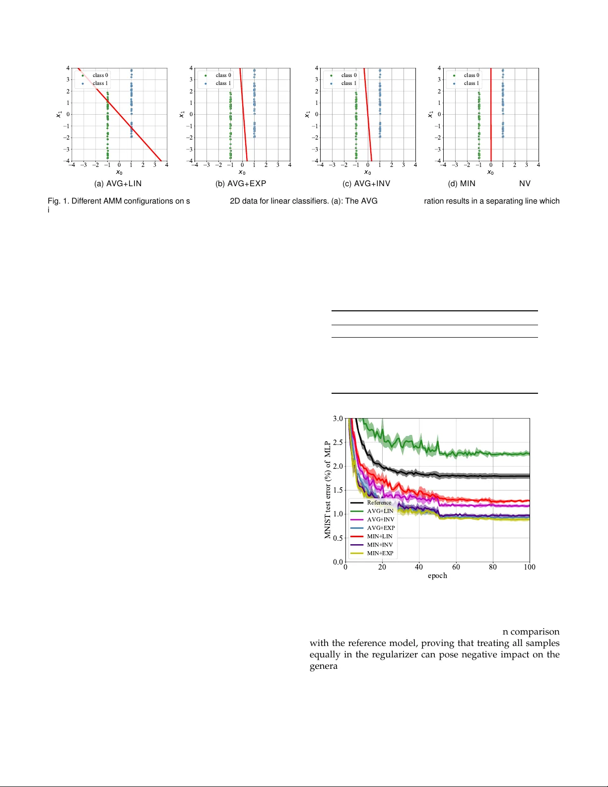
1 Adv ersar ial Margin Maximization Networks Ziang Y an, Yiw en Guo , and Changshui Zhang, Fello w , IEEE Abstract —The tremendous recent success of deep neural networks (DNNs) has sparked a surge of interest in understanding their predictive ability . Unlike the human visual system which is ab le to generalize rob ustly and lear n with little super vision, DNNs normally require a massive amount of data to learn new concepts . In addition, research works also show that DNNs are vulnerab le to adversarial e xamples—maliciously generated images which seem perceptually similar to the natural ones b ut are actually formed to fool learning models, which means the models ha ve prob lem generalizing to unseen data with cer tain type of distor tions. In this paper , we analyze the gener alization ability of DNNs comprehensively and attempt to impro ve it from a geometric point of view . W e propose adversarial margin maximization (AMM), a learning-based regularization which exploits an adversarial perturbation as a proxy . It encourages a large margin in the input space, just lik e the suppor t vector machines. With a diff erentiable formulation of the per turbation, we train the regularized DNNs simply through bac k-propagation in an end-to-end manner. Experimental results on various datasets (including MNIST , CIF AR-10/100, SVHN and ImageNet) and diff erent DNN architectures demonstrate the superiority of our method ov er previous state-of-the-arts. Code and models f or reproducing our results will be made publicly a vailab le. Index T erms —Large margin classifier , adversarial per turbation, generalization ability , deep neural networks F 1 I N T R O D U C T I O N A L though deep neural networks (DNNs) have shown state-of-the-art performance on a variety of challeng- ing computer vision tasks, most of them ar e still ”notorious” for r equiring massive amount of training data. In addition, a bunch of recent works also demonstrate that DNNs are vul- nerable to adversarial examples [1], [2], [3], [4], indicating the models have problem generalizing to unseen data with possible types of distortions [5], [6]. These undesirable facts motivate us to analyze the generalization ability of DNNs and further find a principled way to improve it. Our work in this paper stems specifically fr om a geomet- ric point of view . W e delve deeply into the margin of DNNs and advocate a large margin principle for training networks. Generally , such a principle can enhance the obtained models over two aspects: (a). maximum margin classifiers usually possess better generalization ability , which is both theoret- ically guaranteed and empirically verified [7], [8], [9], [10]; and (b). they can also be naturally more r obust to adversarial examples since it takes more ef forts to perturb the inputs to- wards decision boundaries. This paper substantially extends the work of Y an et al. published at NeurIPS 2018 [11]. The original concept of the large margin principle dates back to last century . Novikof f, Cortes and V apnik pr oved es- sential theorems for the perceptr on [12] and support vector machines (SVMs) [7], based on a geometric mar gin γ and an assumption that the training data can be separated with it: sup w min i y i f ( x i , w ) > γ . (1) • Z. Y an and C. Zhang are with the Institute for Artificial Intelligence, T s- inghua University (THUAI), the State Key Lab of Intelligent T echnologies and Systems, the Beijing National Research Center for Information Sci- ence and T echnology (BNRist), the Department of Automation, T singhua University , Beijing 100084, China. E-mail: yza18@mails.tsinghua.edu.cn; zcs@mail.tsinghua.edu.cn. • Y . Guo is with the Bytedance AI Lab, Beijing, China. E-mail: guoyi- wen.ai@bytedance.com. Unlike the well-known scheme in linear classification [7], the geometric margin of nonlinear DNNs scarcely has close- form solutions, making it non-trivial to get incorporated in the training objective. Although many attempts have been made to pursue this target, most of them just focus on a margin in the repr esentation space (a.k.a, feature space) [13], [14], [15], [16]. Learned representations in such a manner may show better intra-class compactness and inter-class discriminability , but in practice a large margin in the featur e space itself does not necessarily guarantee a large margin in the input space [17], on account of the distance distortions of nonlinear hierarchical models. T o address this pr oblem, several recent methods have been developed to suggest a large margin directly in the input space. For example, An et al. [17] study contractive mappings in DNNs and propose contractive rectifier networks, while Sokoli ´ c et al. [18] try penalizing the Frobenius norm of a Jacobian matrix instead. These methods show significantly superior performance in scenarios where for instance the amount of training data is severely limited. However , aggressive assumptions and approximations seem inevitable in their implementations, making them less effective in practical scenarios where the assumptions are not really satisfied. In this paper , we propose adversarial margin maximiza- tion (AMM), a learning-based regularization that exploits an adversarial perturbation as a proxy of γ . Our core idea is to incorporate an l 2 norm-based adversarial attack into the training process, and leverage its perturbation magnitude as an estimation of the geometric margin. Current state- of-the-art attacks typically achieve ∼ 100% success rate on powerful DNNs [3], [19], [20], while the norm of perturba- tion can be reasonably small and thus fairly close to the real margin values. Since the adversarial perturbation is also pa- rameterized by the network parameters (including weights and biases), our AMM regularizer can be jointly learned with the original objective thr ough back-propagation. W e conduct extensive experiments on MNIST , CIF AR-10/100, SVHN and ImageNet datasets to testify the effectiveness 2 of our method. The results demonstrate that our AMM significantly improves the test-set accuracy of a variety of DNN architectur es, indicating an enhanced generalization ability as the training-set accuracies remain similar . The r est of this paper is organized as follows. In Sec- tion 2, we introduce representative margin-based methods for training DNNs. In Section 3, we highlight our motivation and describe our AMM in detail. In Section 4 we experi- mentally validate the effectiveness of our proposed method. Finally , Section 5 draws the conclusions. 2 R E L AT E D W O R K Margin-based methods have a long research history in the field of pattern recognition and machine learning. Theo- retical relationships between the generalization ability and geometric margin of linear classifiers have been compre- hensively studied [8] and the idea of leveraging large mar- gin principle and constructing maximal margin separating hyperplane [8] also act as essential ingredients of many classical learning machines, c.f. the famous SVM [7]. Benefit fr om its solid theoretical foundation and intuitive geometric explanations, the large margin principle has been widely applied to a variety of real-world applications such as face detection [21], text classification [22], gene selection for cancer classification [23], etc. Nevertheless, there is as of yet few methods for applying such principle to DNNs which are ubiquitous tools for solving modern machine learning and pattern recognition tasks (but are also structurally very complex and generally considered as black-boxes). This is mostly because the margin cannot be calculated analytically in general as with SVM. In view of such opportunities and challenges, one line of researches targets at improving a ”margin” in the repre- sentation space of DNNs instead. For instance, T ang [13] re- places the final softmax layer with a linear SVM to maximize a margin in the last layer . Hu et al. [14] propose a discrimina- tive learning method for deep face verification, by enfor cing the distance between each positive pair in the repr esentation space to be smaller than a fixed threshold, and that to be larger than another threshold for all negative pairs, where a margin is naturally formed. A similar strategy , first invented by W einberger et al. [24] and dubbed as triplet loss, has also been widely adopted to many face r ecognition systems, e.g., FaceNet [25]. Sun et al. [26] theoretically study a margin in the output layer of DNNs, and propose a way of reducing empirical margin errors. In the same spirit, W ang et al. [16] propose to further enhance the discriminability of DNN features via an ensemble strategy . Stick with the representation space, some recent works also advocate large margins under differ ent “metrics”, e.g., cosine similarity [27] and the angular distance between logit vectors and the ground-truth [15], [28], [29]. In essence, these methods maximize the inter-class variance while minimiz- ing the intra-class variance, and thus the learned represen- tations can be more discriminative. However , as pr eviously discussed [17], owing to the high structural complexity of DNNs and possible distance distortions of nonlinear mod- els, a large margin in the feature space does not necessarily assure a large margin in the input space. That being said, the aforementioned benefits in Section 1 are not guaranteed. See section 4 for some empirical analyses. It is also worthy of mentioning that some previous works suggest that DNNs trained using stochastic gradients converge to large margin classifiers, but the convergence speed is very slow [30], [31]. A few attempts have also been made towards enlar ging the margin in input spaces. In a recent work, An et al. [17] propose contractive rectifier networks, in which the input margin is proved to be bounded from below by an output margin which is inherently easier to optimize by leveraging off-the-shelf methods like SVM. Sokoli ´ c et al. [18] reveal connections between the spectral norm of a Jacobian matrix and margin, and try to r egularize a simplified version of its Frobenius norm. Contemporaneous with our work, Elsayed et al. [32] propose to use a one-step linear approximation to DNN mappings and enlarge the margin explicitly . These methods are closely related to ours, but their implementa- tions requir e rough approximations and can be suboptimal in many practical applications. Some detailed discussions are deferr ed to Section 3.3.4 and experimental results for comparing with them will be provided in Section 4. Ding et al. [33] also aim to approximate the margin more accurately but their method differs with ours in multiple ways as will be discussed in the Appendix. 3 A D V E R S A R I A L M A R G I N M A X I M I Z AT I O N In this section, we introduce our method for pursuing large margin in DNNs. First, we briefly review our recent work of deep defense [11] aimed at training DNNs with improved adversarial robustness. W e believe its functionality can be naturally regar ded as maximizing the margin. W e then for- malize the definition of margin and provide discussions of the generalization ability based on it. Finally , we introduce our AMM for impr oving the generalization ability of DNNs. 3.1 Our Deep Defense Deep Defense impr oves the adversarial r obustness of DNNs by endowing models with the ability of learning from attacks [11]. On account of the high success rate and rea- sonable computation complexity , it chooses DeepFool [3] as a backbone and tries to enlarge the l p norm of its perturba- tions. 1 Suppose a binary classifier f : R m → R , where the input x is an m -dimensional vector and the predictions are made by taking the sign of classifier ’s outputs. DeepFool generates the perturbation ∆ x with an iterative procedur e. At the i - th step ( 0 ≤ i < u ), the perturbation r ( i ) is obtained by applying first-order approximation to f and solving: min r k r k p s . t . f ( x + ∆ ( i ) x ) + ∇ f ( x + ∆ ( i ) x ) T r = 0 , (2) where ∇ f denotes ∂ f ( x ) ∂ x , and ∆ ( i ) x := P i − 1 j =0 r ( j ) . Problem (2) can be solved analytically: r ( i ) = − f ( x + ∆ ( i ) x ) k∇ f ( x + ∆ ( i ) x ) k 2 2 ∇ f ( x + ∆ ( i ) x ) . (3) 1. There exist stronger attacks which approximate the margin mor e precisely (like the Carlini and W agner ’s [19]), but they are computation- ally more complex; we have demonstrated that defending DeepFool helps to defend Carlini and W agner ’s attack [11] as well ther efore it can be a reasonable proxy . 3 After computing all the r ( i ) s sequentially , the final DeepFool perturbation ∆ x is obtained by adding up the r ( i ) s obtained from each step: ∆ x = r (0) + ... + r ( u − 1) , (4) where u is the maximum iteration allowed. If the prediction class of f changes at any iteration before the u -th, the loop should terminate in advance. Such procedur e directly generalizes to multi-class cases, as long as a target label is properly chosen at each iteration. Given a baseline network, the pr ocedure may take about 1-3 iterations to converge on small datasets such as MNIST/CIF AR-10, and 3-6 iterations on large datasets like ImageNet [34] 2 . 3.1.1 Regularization and High Order Gradients In fact, the ` p norm of ∆ x is a popular metric for evaluating the adversarial attacks and the robustness of DNNs [3], [19], [35]. Given an input vector x , the gradient ∇ f ( x ) , as well as the perturbation ∆ x , are both parameterized by the learnable parameters of f . Consequently , in order to give prefer ence to those f functions with stronger robustness, one can simply penalize the norm of ∆ x as a regularization term during training. W ith modern deep learning frame- works such as PyT or ch [36] and T ensorFlow [37], differ enti- ating ∆ x can be done via automatic derivation with higher order gradients. One might also achieve this by building a “reverse” network to mimic the backward process of f , as described in [11]. W e emphasize the high order gradients form an essential component in our method and. In principle, if no gradient flows through ∇ f , the regularization can be viewed as max- imizing the norm in a normalized logit space, given k∇ f k as the normalizer . Considering possible distance distortions of nonlinear hierarchical DNNs, it is definitely less effective in influencing the perturbation or whatever else. Experimental analysis will be further given in Section 4.3.1 to verify the importance of the high order gradients. 3.1.2 Correctly and Incorrectly Classified Samples Deep Defense applies differ ent regularization strategies on correctly and incorrectly classified samples. Specifically , if an input is correctly classified during training, we expect it to be pushed further away from the decision boundary , thus a smaller value of k ∆ x k p is anticipated. In practice, the target class at each iteration is chosen to be the one results in the smallest r ( i ) . Conversely , if an input is misclassified by the current model, we instead expect it to be closer to the decision boundary (between its current prediction and the ground-truth label), since we may intuitively hope the input sample to be correctly classified by the model in the future. The target class is always set to be the ground-truth and a larger value of k ∆ x k p is anticipated. In summary , the Deep Defense regularizer can be written as: L DD = X k ∈T R  − c k ∆ x k k p k x k k p  + X k ∈F R  d k ∆ x k k p k x k k p  , (5) 2. For example, it convergences within 3 iterations on all the MNIST images with a 5-layer LeNet reference model, and 6 iterations on 99.63% of the ImageNet images with a ResNet-18 reference model. or similarly L DD = 1 n X k ∈T R ( − c k ∆ x k k p ) + 1 n X k ∈F R ( d k ∆ x k k p ) , (6) where n is the number of training samples, T is the index set of correctly classified training examples, F is its comple- ment, c, d > 0 are two hyper-parameters balancing these two groups of samples, R is the shrinkage function that balances examples within the same group (details in Section 3.3). The sets T and F are updated in each training iteration. The whole optimization problem is given by: min W X k L ( y k , f ( x k ; W )) + λL DD + αL W D , (7) where L is the original classification objective (e.g., cross- entropy or hinge loss), λ is the coefficient for regularizer , and αL W D is the weight decay term. W e adopt the unnor- malized version (6) in this paper , since it connects the most to the margin to be defined in Section 3.2, and further the generalization ability . 3.2 Margin, Rob ustness and Generalization Deep defense achieves r emarkable performance on r esist- ing different adversarial attacks. Apart from the improved robustness, we also observe increased inference accuracies on the benign test-sets (cf., the fourth column of T able 1 in the paper [11]). W e believe the superiority of our inference accuracies is related to the nature of large margin principle. In order to analyze the conjectur e in detail, we first formalize the definition of an instance-specific margin and introduce some prior theoretical results [10] as below . Definition 3.1. Let us denote by g : R m → {± 1 } a decision function, then the instance-specific margin γ p x of a sam- ple x ∈ R m w .r .t. g is the minimal ` p distance fr om x to the decision boundary . Definition 3.2. [10] Let S n be a sampled training set, and l be the loss function. An algorithm is ( K ,  ( S n )) -robust if the sample space S = X × Y can be partitioned into K disjoint sets denoted by K k , k = 1 , . . . , K , such that for all s j = ( x j , y j ) ∈ S n and s = ( x , y ) ∈ S , s j , s ∈ K k ⇒ | l ( g ( x j ) , y j ) − l ( g ( x ) , y ) | ≤  ( S n ) . (8) Theorem 3.1. [10] If there exists 0 < γ p < γ p x j for all j , then the learning algorithm is (2 N ( γ p / 2 , X ; d p ) , 0) -robust, in which N ( γ p / 2 , X ; d p ) is the  -covering number 3 of the input space X , and d p is the ` p norm, in which the 0/1 loss l ( g ( x j ) , y j ) = 1 ( g ( x j ) 6 = y j ) is chosen. Theorem 3.1 establishes an intrinsic connection between the concerned instance-specific margin and a defined “ro- bustness”. Such robustness is differ ent from the adversarial robustness by definition, but it theoretically connects to the generalization error of g , as shown in Theorem 3.2. Theorem 3.2. [10] Let µ be the underlying distribution of the sample ( x , y ) . If an algorithm is ( K ,  ( S n )) -robust and 3. The definition of  -covering number can be found in [38], and it is monotonically decreasing w .r .t. its first argument. 4 l ( g ( x ) , y ) ≤ M for all s = ( x , y ) ∈ S , then for any δ > 0 , with probability at least 1 − δ , it holds that GE( g ) ≤  ( S n ) + M s 2 K log(2) + 2 log (1 /δ ) n , (9) in which GE( g ) is the generalization error of g , given by GE( g ) =       E ( x ,y ) ∼ µ l ( g ( x ) , y ) − 1 n X ( x j ,y j ) ∈S n l ( g ( x j ) , y j )       . (10) Theorem 3.2, along with Theorem 3.1, advocates a large margin in the input space and guarantees the generalization ability of learning machines. Also, it partially explains the superiority of our Deep Defense trained DNNs on benign- set infer ence accuracies. However , since the r egularizer L DD is originally designed for resisting attacks, it may be subop- timal for improving the generalization ability (or reducing the generalization error) of learning machines. In fact, for linear binary classifiers where f ( x ) = w T x + b , assuming the training data is fully separable, then the regularization boils down to minimizing 4 : X k ∈T −   w T x k + b   k w k 2 + X k ∈F   w T x k + b   k w k 2 . (11) Since scaling ( w , b ) by any positive scalar t does not change the value of our r egularization term, we constrain k w k 2 = 1 to make the problem well-posed. W e denote the index set of samples from positive class and negative class by S + n and S − n , respectively , and further assume the number of training samples in positive and negative classes to be identical (i.e., |S + n | = |S − n | ), then Eq. (11) can be rewritten as: w T   X k ∈S − n x k − X k ∈S + n x k   , (12) in which the bias term b has been canceled out. Obviously , minimizing Eq. (12) under the constraint k w k 2 = 1 yields w ∗ = ( P k ∈S + n x k − P k ∈S − n x k ) / Z , where Z is a normal- izer to make sure k w ∗ k 2 = 1 . Geometrically , the decision boundary corresponding to calculating w ∗ is orthogonal to the line segment connecting the centers of mass of positive training samples and that of negative training samples. Note that all training samples in (12), no matter how far away from the decision boundary , have equal contribution to w ∗ . An undesired consequence of such formulation is that, the regularizer can be severely influenced by samples not really close to the decision boundary . As a result, such w ∗ may process a poor global margin γ p , since γ p is generally the “worst-case” distance from training samples to the decision boundary , dominated mainly by those close to it. 3.3 Our Main Framew ork W e know from the previous section that although the mar- gin, r obustness and generalization ability of DNNs are theo- retically connected, there is an intrinsic distinction between our current method and a desired margin maximization. In 4. W e choose λ = c = d = 1 , and R ( t ) = t for simplicity . this section, we provide further analyses and introduce ag- gregation function (in Section 3.3.1) and shrinkage function (in Section 3.3.2) designed specifically to exploit the large margin principle more effectively in practice. 3.3.1 Aggregation Function Deep Defense in Eq. (6) aggregates regularization informa- tion from training samples (in a batch) by taking average. However , this aggregation strategy can be suboptimal for improving the generalization ability , while Theorem 3.2 also suggests a minimal perturbation (rather than the adopted average). Ideally , one can apply regularization only on the sample with minimal perturbation over the whole training set to maximize γ p = min j γ p x j . Nevertheless, the gradient of such a regularizer will be zero for most of the training samples, and in practice it takes much longer time to train and achieve satisfactory results. This is different from the well- known scheme in linear SVM. T o achieve a reasonable trade-of f between the theoretical requir ement and regularization strength, we consider using a M I N aggregation function within each batch instead of the whole training set during training. Specifically , for correctly classified samples x k we apply regularization to it iff two conditions are fulfilled simultaneously: (a). k ∆ x k k is the smallest among all samples with the same ground-truth label in this batch, and (b). k ∆ x k k belongs to the top 20% smallest in this batch. If a correctly classified sample does not satisfy these two conditions, we simply set its regular- ization term to zero in the current training step. While if a sample is misclassified by the current model, we expect to decrease its distances to the correct predictions. Analogous to the above codec for M I N, we denote the original Deep Defense strategy (i.e., averaging all) as A V G . 3.3.2 Shrinkage Function As discusses [11], if we penalize an perturbation directly (i.e., setting R ( t ) = t in Eq. (5) and (6)), some “extremely robust” samples may dominate the r egularization term, which shall pose a negative impact on the training pro- cedure. What’s worse, the regularization term will never diminish to zero with a linear R ( · ) . T o alleviate the prob- lems, we attempt to choose a nonlinear ”shrinkage” func- tion for R ( · ) . It should be monotonically increasing, such that the correctly classified samples with abnormally small k ∆ x k k are penalized more than those with relatively large values. Essentially , concentrating mor e on samples with small instance-specific margins coheres with the evidence in Theorem 3.2, since we know the minimal (instance-specific) margin probably connects the most to the generalization ability . W e will demonstrate the performance of differ ent choices: (a). R ( t ) = t , denoted by L I N , (b). R ( t ) = exp( t ) , denoted by E X P and (c), R ( t ) = 1 1 − t , denoted by I N V , on training DNNs, which also differs from the well-known scheme in linear SVM. For I N V , we make sur e t < 1 by setting appropriate values for c, d and truncating abnormally large values for k ∆ x k k with a threshold. 3.3.3 Experiments on T oy Data W e first conduct an explanatory experiment by synthesizing 2D data to illustrate how the choices of the functions may af- fect classification in a binary case. Suppose that the 2D data 5          x 0          x 1     (a) AVG + L I N          x 0          x 1     (b) AVG + E X P          x 0          x 1     (c) AVG + I N V          x 0          x 1     (d) M I N + L I N / E X P / I N V Fig. 1. Different AMM configurations on synthesiz ed 2D data f or linear classifiers. (a): The AVG + L I N configuration results in a separating line which is or thogonal to the line connecting the centers of different classes. (b), (c): By adjusting the scales of regularization ter m of different data points using our non-linear shrinkage functions, we obtain decision boundaries with improv ed margins and better generalization ability compared with the linear shr inkage function adopted in AVG + L I N. (d): When the regular ization is only applied to samples with small (instance-specific) margins, the learned models almost show optimal performance up to the limit on numerical precisions. The decision boundar ies are plotted in red. Best viewed in color . from the two classes ar e uniformly distributed in rectan- gles [ − 1 . 01 , − 4 . 00; − 0 . 99 , 2 . 00] and [0 . 99 , − 2 . 00; 1 . 01 , 4 . 00] , respectively . For each class, we synthesize 200 samples for training and another 200 held-out for testing. W e train linear classifiers with f ( x ) = w T x + b to minimize the regular- ization term taking various forms. W e set batch size to 20, and train models for 1000 epochs with the standar d SGD optimizer . The learning rate is initially set to 0.1, and cut by half every 250 epochs. W e use the popular momentum of 0.9 and a weight decay of 1e-4. The learned decision boundaries and in differ ent config- urations are illustrated in Fig. 1 together with test samples. W ith purely A V G + L I N , the obtained boundary is roughly orthogonal to the line connecting (-1.0, -1.0) and (1.0, 1.0), which is consistent with our previous analysis in Section 3.2. Although we have striven to penalize incorrect classifica- tions, the obtained model in this setting is still unable to gain excellent accuracy , because all training samples contribute equally to pushing the decision boundary . Better general- ization ability and thus improved test-set accuracies can be obtained in the A V G + E X P and A V G + I N V settings, as depicted in Fig. 1 (b) and (c). This verifies the effectiveness of the non-linear shrinkage functions aimed at regularizing ”extremely robust” samples less. It can also be seen that the M I N aggregation function leads to a more sensible margin. Optimal (or near optimal) boundaries are obtained in the MIN settings, which attains the largest possible margin of 1. As discussed in Section 3.2, the M I N aggregation function is more r elated with the geometric margin in comparison with the A V G so it can directly facilitate the margin as well as the generalization ability . W e further conduct an experiment on MNIST [39], which is a real-world dataset. Here a simple multilayer perceptron (MLP) is adopted and trained with cross-entropy loss. T o achieve the best performance within each configuration, we first run a grid search for λ , c , and d . T able 1 shows the final error rates while Fig. 2 illustrates the convergence curves of our AMM with differ ent aggregation and shrinkage func- tions. W e repeat the training five times with differ ent initial- ization instantiations to report also the standard derivations of error rates. W e see with A V G + L I N the obtained mean T ABLE 1 Results on MNIST: Compare MLP Models T rained Using Different Aggregation and Shrinkage Functions Method Aggregation Shrinkage Error Rate (%) baseline - - 1.79 ± 0.06 A V G L I N 2.26 ± 0.05 A V G I N V 1.18 ± 0.03 AMM A V G EX P 0.94 ± 0.02 M I N L I N 1.28 ± 0.02 M I N I N V 0.97 ± 0.03 M I N E X P 0.90 ± 0.03                             Fig. 2. Conv ergence cur ves of MLP models trained using our AMM with different agg regation and shrinkage functions on MNIST . error rate even incr eases from 1.79% to 2.29% in comparison with the reference model, proving that treating all samples equally in the regularizer can pose negative impact on the generalization ability . W ith the help of the M I N aggregation function, our AMM achieves a 1.28% error rate, which is far lower than that with A V G + L I N (2.26%), as well as that of the refer ence model (1.79%). Such positive effect of the M I N aggregation function is consistent with our observation on the synthetic 2D data. The benefit of the nonlinear shrinkage functions is also 6 highlighted. When compared with the L I N function, non- linear shrinkage functions I N V and E X P gain relative error decreases of 47% and 58% within the same A V G setting, and 24% and 29% within the M I N setting. Such results well explain our intuitions and insights in Section 3.3.2. 3.3.4 Implementation Details and Discussions Our framework has an intrinsic connection with SVM. For a linear binary classification problem with separable training data, SVM can be viewed as a special case in our framework provided the model is linear , if we remove the classification objective L in the whole optimization problem (7). It can be easily verified that the M I N + L I N r egularization (along with the weight decay term) is the equivalent with a hard mar gin linear SVM, if the curr ent model achieves excellent accuracy (i.e.100%) on the training set and we use all training samples in each batch. Moreover , as testified in the previous section, the aggregation function ought to be mor e essential than the shrinkage function in linear binary cases. The landscape and margin of nonlinear DNNs are much more complex and generally infeasible to compute in com- parison with those of linear models, especially when multi- ple classes get involved. Our framework exploits an adver- sarial perturbation as a proxy of the margin. W ith differ ent configurations on the aggregation and shrinkage functions, it formulates a variety of regularization types. They might devote more to the generalization ability (e.g., the one with M I N + E X P) or robustness (e.g., our Deep Defense with A V G and approximately E X P). All the encompassed variants share a similar core idea that is to incorporate an adversarial attack into the training process. In particular , we utilize the perturbation norm as an estimation of the margin. Current state-of-the-art attacks typically achieve ∼ 100% success rate on powerful DNNs, while the norm of perturbation can be reasonably small and thus fairly close to the r eal margin values. W e specifically choose p = 2 to comply with previ- ous theoretical analysis. Also, we know from Section 3.3.3 that the M I N + E X P trades off test-set performance in favor of theoretical margins. W e leave the choices for the classi- fication objective L to customized network configurations, in parallel with our AMM configurations. In fact, we have tested our AMM with popular choices for L including the cross-entr opy loss and hinge loss but never found a significant differ ence in the experiments. By delving deeply into the geometric margin, we unify a set of learning-based regularizers within the proposed AMM framework. Guidelines ar e correspondingly provided in case one prefers the generalization ability to robustness or DNNs to linear models. Contemporaneous with our work, Elsayed et al. [32] propose to linearize the forward mapping of DNNs, somewhat similar to a single-step Deep Defense without utilizing the high order gradients (as in Section 3.1) and nonlinear shrinkage function (as in Section 3.3.2). See more discussions in Section 4.3.1. 4 E X P E R I M E N TA L V E R I FI C AT I O N S In this section, we experimentally verify the remarks and conjectures presented in previous sections and evaluate the performance of our AMM with specifically M I N + E X P on various datasets (including MNIST , CIF AR-10/100, SVHN and ImageNet). W e compare our derived method with the state-of-the-arts to demonstrate its effectiveness. 4.1 Datasets and Models W e perform extensive experiments on five commonly used classification dataset: MNIST [39], CIF AR-10/100 [40], SVHN [41] and ImageNet [34]. Dataset and network config- urations are described as below . For MNIST , CIF AR-10/100, and SVHN, we constr uct a held-out validation set for hyper- parameter selection by randomly choosing 5k images from the training set. For ImageNet, as a common practice, we train models on the 1.2 million training images, and report top-1 error rates on the 50k validation images. 4.1.1 MNIST MNIST consists of 70k grayscale images, in which 60k of them are used for training and the remaining are used for test. W e train deep networks with dif ferent architectur es on MNIST : (a). a four-layer MLP (2 hidden layers, 800 neurons in each) with ReLU activations, (b). LeNet [39] and (c). a deeper CNN with 12 weight layers named “LiuNet” [15], [16]. Similar to many previous works, we subtract the mean for both training and test data in pre-processing, and no data augmentation is adopted. For more details about these architectur es, please see our appendix. 4.1.2 CIF AR-10/100, and SVHN Both CIF AR-10 and CIF AR-100 contain 60k color images, including 50k training images and 10k test images. SVHN is composed of ∼ 630k color images in which ∼ 604k of them are used for training and the remaining for testing. For these datasets, we train six networks: (a). a light ConvNet with the same ar chitecture as in [42], (b). the network-in- network (NIN) [43], (c). the “LiuNet“ as applied in the CIF AR-10 experiments in [15]., (d)(e). the standar d ResNet- 20/56 [44] ar chitectures, and (f) a DenseNet-40 [45] in which all layers are connected. W e uniformly resize each image to 36x36, and randomly crop a 32x32 patch during training as data augmentation. Moreover , we apply random horizontal flipping with a probability of 0.5 to combat overfitting, except SVHN. 4.1.3 ImageNet ImageNet is a highly challenging image classification bench- mark which consists of millions of high-resolution images over 1,000 classes. Starting from ResNet [44], deep models with skip connections have advanced the state-of-the-arts on this highly challenging dataset [45], [46], [47], [48]. W e adopt ResNet-18/50 [44] and SENet-50 [48] which includes numerous skip connections as representative architectures to validate our method. Following previous works [49], we randomly crop a patch whose size is uniformly distributed between 8% and 100% of the original image size, with aspect ratio uniformly distributed in  3 4 , 4 3  . Then we resize the cropped patch to 224x224 and feed it into the network. As a common practice, random horizontal flipping is also applied. 7 T ABLE 2 MNIST T est Error Rates of MLP Models w/ or w/o High Order Gradients Model Error (%) Reference 1.79 ± 0.06 w/o high order gradients 1.46 ± 0.04 w/ high order gradients 0.90 ± 0.03 4.2 T raining Protocol W e use the cross-entropy loss in the training objective for L , as wit h pr evious works. T able 2 in the appendix summarizes the batch size, maximal number of epoch, and learning rate policy used in our experiments. W e start training with some initial learning rate (shown in the 5-th column of T able 2) and we anneal them by some multipliers at certain epochs (specified in the 6-th column). The standard stochastic gradi- ent descent optimizer with a momentum of 0.9 and a weight decay of 1e-4 is adopted in all experiments. All the hyper- parameters are tuned on the validation set with reference networks in order to achieve their supreme performance. For r elatively small models and datasets, we initialize models with the so-called “MSRA ” strategy [50] and train from scratch, otherwise we fine-tune from our trained ref- erence models (more details can be found in T able 2 in the appendix). T o avoid abnormally large gradients and proba- bly a drift away of classification loss, we project gradient tensors onto a Euclidean sphere with radius 10, if their norm exceeds the threshold 10. This technique is also known as “clip gradients” and has been widely adopted in the community . When calculating adversarial perturbations for our AMM, we allow a maximal iteration of u = 6 , which is sufficient to fool DNNs on ∼ 100% of the training samples in most cases. Hyper-parameters λ, c, d in our regularizer is determined by cross validation in the held-out validation set, as described. 4.3 Exploratory Experiments on MNIST As a popular dataset for evaluating the generalization per- formance of classifiers [13], [15], [17], [42], [51], MNIST is a reasonable choice for us to get started. W e shall analyze the impacts of differ ent configurations in our framework. 4.3.1 Eff ect of High Order Gradients and Others Let us first investigate the effect of introducing high order gradients, which serves as an essential component in our framework. It is triggered when back-pr opagating gradients through ∇ f in our regularizer , which is usually difficult to formalize and compute for DNNs. W e invoke the automatic differ entiation mechanism in PyT orch [36] to achieve this. One can also build inverse networks to mimic the backward process of DNNs, as in [11]. W e try masking the gradient flow of ∇ f by treating the entries of ∆ x as constants, as done by Elsayed et al. [32]. In general, they expect to enlarge the margin by penalizing the ` 2 norm of a linear perturbation, if it goes below a threshold. Such approximation may lead to conceptually easier imple- mentations but definitely also results in distinctions fr om the gradient direction to pursue a large margin. W ith or without the high order gradients, we obtain different MLP                                 Fig. 3. Conv ergence cur ves of MLP models on MNIST with or w/o high order gradients . models using our AMM. They are compared in T able 2 and Fig. 3, along with the “Reference” that indicates t he baseline MLPs with λ = 0 (i.e., no AMM). Means and standard deviations of the error rates calculated fr om all five runs are shown. Though both methods achieve decr eased error rates than the “Reference”, models trained with gradient masked on ∇ f (i.e., without high order gradients) demonstrate appar- ently worse performance (1.46%, pink in Fig. 3) than those with full gradients (0.90%, yellow in Fig. 3). Except for the high or der gradients, Elsayed et al.’s method [32] also miss several other components that may further hinder it from achieving comparable performance with ours. For empirical validations, we try following its main technical insights and implementing the method for empirical validation. W e fol- low the single-step setting and a threshold-based shrinkage function and summarize its results in T able 2 and Fig. 3 for comparison. W e see its prediction error is even higher than ours without high order gradients. 4.3.2 T raining with Less Samples Our AMM enhances the generalization ability and robust- ness of DNNs in different aspects. W e consider the pos- sibility of training DNN models with fewer samples in this section. Specifically , we sample { 5k , 10k , 15k , . . . , 60k } images randomly from the MNIST training set, and train MLP models on these subsets. Once sampled, these subsets are fixed for all training procedures. The M I N + E X P setting and identical λ , c , and d as in our pr evious experiments are adopted. Fig. 4 illustrates how test error rates vary with the num- ber of training samples. Same with previous experiments, we perform five runs for each method and the shaded areas demonstrate the standard deviations. Clearly , models with our full gradient AMM achieve consistently better perfor- mance than the “Reference” models and other competitors. W ith only 20k training images, our method helps to achieve 1 . 54 ± 0 . 04% err or , which is even slightly lower than that of the vanilla models with all 60k training images ( 1 . 81 ± 0 . 05% error). 8                              Fig. 4. MNIST test error rates of MLP models with less training images . 4.3.3 T raining with Noisy Labels W e train models with possibly noisy labels in this exper- iment to simulate unreliable human annotations in many real-world applications. W e shall use all 60k MNIST training images, but for a portion of them, we substitute random integers in [0, 9] for their “ground-tr uth” labels. For n ∈ { 0k , 5k , 10k , . . . , 55k } , we construct 12 training partitions each consists of n images with the original labels and 60k − n images with random labels. The “Reference” and our AMM models are trained, and their error rates ar e shown in Fig. 5. W ithout specific r egular- ization, error rates of refer ence models increase drastically when a portion of labels are corrupted. For instance, when training on a set containing 55k images with random labels, models with our adversarial regularization are still able to achieve an average test err or less than 10%. However , that of the reference models goes above 40%, which are obviously too high, considering it is a 10-class classification problem. Our implementation of Elsayedet al.’s method also achieves promising performance on the test set, though consistently inferior to ours. 4.4 Image Classification Experiments In this section, we testify the ef fectiveness of our method on benchmark DNN architectur es on different image clas- sification datasets including MNIST , CIF AR-10/100, SVHN and ImageNet. It is compared with a variety of state- of-the-art margin-inspir ed methods. Same with previous experiments in Section 4.3, during training we adopt the M I N + E X P regularizer in our method for all experiments. For evaluation, both error rates and mar gin (estimated using DeepFool perturbation) on the test set are reported to verify the effectiveness of our method. 4.4.1 MNIST Aforementioned MLP , LeNet and LiuNet architectur es are used as reference models. Generally , DNNs have to be de- terministic during the attack process, such that we can find a reasonable appr oximation of minimal distance to the fixed decision boundaries. However , for DNNs equipped with                                Fig. 5. MNIST test error rates of MLP models with noisy training images. T ABLE 3 MNIST T est Error Rates Method Architecture Error (%) Margin Augmentation Bayes by Backprop [51] MLP (800) 1.32 - - DropConnect [52] MLP (800) 1.20 ± 0.03 - - DLSVM [13] MLP (512) 0.87 - Gaussian CRN [17] LeNet 0.73 - - DropConnect [52] LeNet 0.63 ± 0.03 - - DisturbLabel [42] LeNet 0.63 - - L-Softmax [15] LiuNet 0.31 - - EM-Softmax [16] LiuNet 0.27 a - - Reference MLP (800) 1.79 ± 0.06 0.76 - Ours MLP (800) 0.90 ± 0.03 1.90 - Reference LeNet 0.87 ± 0.02 1.07 - Ours LeNet 0.56 ± 0.02 2.21 - Reference LiuNet 0.41 ± 0.02 1.60 - Ours LiuNet 0.33 ± 0.03 3.41 - a Ensemble of 2 LiuNet models are used. batch normalization layers, if we implement the DeepFool attack na ¨ ıvely , the perturbation of a particular sample may depend on other samples in the same batch since all of them share the same mean and variance in batch normalization procedur e. In order to bypass such dependency and achieve better efficiency , our implementation follows that described in [15], with one exception that we replace all batch nor- malization layers with group normalization [53] with group size 32. Empirically we found this difference has little (often negative) impact on the error rates of refer ence network. W e adopt the M I N + E X P setting, and use λ , c , d selected on MLPs for all the three ar chitectures for simplicity , although potential better hyper-parameters may be obtained by run- ning grid sear ch on each of them. The error rates of dif ferent methods are shown in T able 3. For a fair comparison, we also provide architectur es in the second column of T able 3. The annotation MLP ( n ) represents an MLP model with two hidden layers, and each of them has n neur ons. Our method outperforms competitive methods considering the MLP and LeNet architectur e, except one case where comparisons are not completely fair: DLSVM [13] obtains 0.87% error (our: 0.90%) using MLP with additional Gaussian noise added to the input images during training, but we do not use any data augmentation techniques,. For LiuNet, our method also achieves comparable error rate (0.33%) with L-Softmax [15] (0.31%). EM-Softmax [16] achieves the lowest 0.27% error 9 T ABLE 4 CIF AR-10 T est Error Rates Method Architecture Error (%) Margin Augmentation DropConnect [52] LeNet 18.7 - - DisturbLabel [42] LeNet 14.48 - hflip & crop DLSVM [13] LeNet 11.9 - hflip & jitter CRN [17] VGG-16 8.8 - hflip & crop L-Softmax [15] LiuNet 5.92 - hflip & crop EM-Softmax [16] LiuNet 4.98 a - hflip & crop Reference LeNet 14.93 0.16 hflip & crop Ours LeNet 13.87 0.24 hflip & crop Reference NIN 10.39 0.21 hflip & crop Ours NIN 9.87 0.30 hflip & crop Reference LiuNet 6.25 0.15 hflip & crop Ours LiuNet 5.85 0.29 hflip & crop Reference ResNet-20 8.20 0.10 hflip & crop Ours ResNet-20 7.62 0.22 hflip & crop Reference ResNet-56 5.96 0.16 hflip & crop Ours ResNet-56 5.75 0.32 hflip & crop Reference DenseNet-40 5.75 0.11 hflip & crop Ours DenseNet-40 5.61 0.18 hflip & crop a Ensemble of 2 LiuNet models are used. using an ensemble of 2 LiuNets, while our performance is measured on a single model. Mor eover , we see our method significantly and consistently decreases the error rates of refer ence models, by relative improvements of 49%, 35%, and 19% on MLP , LeNet, and LiuNet, respectively . 4.4.2 CIF AR-10 For CIF AR-10, we evaluate our method with LeNet, NIN, LiuNet, ResNet-20/56, and DenseNet-40. The architectur e of LeNet and NIN are directly copied from our pr evi- ous work [11], and that of LiuNet is adapted from [15]. W e choose the CIF AR-10 LiuNet architectur e as described in [15], and replace all batch normalization layers with group normalization layers of group size 32, as in our MNIST experiments. For ResNets and DenseNets, we adopt the standard architectur es as described in previous works [44], [45], and simply freeze all batch normalization layers during both training and testing to break the the inter-batch dependency as described in Section 4.4.1. Hyper- parameters λ , c , and d are casually tuned on the hold- out validation set as described in Section 4.1, and final error rates ar e reported using models trained on the full training set of 50k images. T able 4 summarizes results for CIF AR-10 experiments. For fair comparison we also show data augmentation strategies in the last column of T able 4. Majority of methods use horizontal flip and random crop, while T ang et al. [13] use horizontal flip and color jitter , which may partially explain the surprisingly low error rate (11.9%) obtained with LeNet. In most test cases considering the same architecture and data augmentation strategy , our regularizer produces lower error rates than all other com- petitive methods. The only exception is EM-Softmax with LiuNet, which achieves 4.98% error (ours 5.85%). However , their result is obtained on an ensemble of 2 LiuNet models, while our results are measured on a single LiuNet model without any ensemble. Moreover , it can be seen that our method also provides significant absolute improvements to all six refer ence models with different architectures. 4.4.3 CIF AR-100 Similar to the CIF AR-10 experiment, we also evaluate our method on LeNet, NIN, LiuNet, ResNet-20/56, and T ABLE 5 CIF AR-100 T est Error Rates Method Architectur e Error (%) Margin Augmentation DisturbLabel [42] LeNet 41.84 - hflip & crop CRN [17] VGG16 34.4 - - L-Softmax [15] LiuNet 29.53 - - L-Softmax [15] LiuNet 28.04 a - hflip & crop EM-Softmax [16] LiuNet 24.04 b - hflip & crop Reference LeNet 43.30 0.11 hflip & crop Ours LeNet 41.68 0.23 hflip & crop Reference NIN 37.75 0.12 hflip & crop Ours NIN 34.49 0.21 hflip & crop Reference LiuNet 26.87 0.10 hflip & crop Ours LiuNet 25.91 0.18 hflip & crop Reference ResNet-20 33.20 0.05 hflip & crop Ours ResNet-20 32.96 0.16 hflip & crop Reference ResNet-56 26.70 0.06 hflip & crop Ours ResNet-56 26.54 0.14 hflip & crop Reference DenseNet-40 25.93 0.04 hflip & crop Ours DenseNet-40 25.62 0.11 hflip & crop a W e copy the r esult from a non-of ficial implementation [16], since the original paper [15] does not provide such result for CIF AR-100 with data augmentation. b Ensemble of 2 LiuNet models are used. T ABLE 6 SVHN T est Error Rates Method Architectur e Error (%) Margin Augmentation DisturbLabel [42] LeNet 3.27 - crop Reference LeNet 3.32 0.45 crop Ours LeNet 3.12 0.99 crop Reference NIN 2.67 0.48 crop Ours NIN 2.46 1.14 crop Reference LiuNet 1.79 0.50 cr op Ours LiuNet 1.61 1.24 crop Reference ResNet-20 1.91 0.40 cr op Ours ResNet-20 1.82 1.17 cr op Reference ResNet-56 1.72 0.54 cr op Ours ResNet-56 1.63 1.04 cr op Reference DenseNet-40 1.79 0.46 crop Ours DenseNet-40 1.66 0.99 crop DenseNet-40 for CIF AR-100. LeNets, NINs, ResNets and DenseNets are kept the same with the CIF AR-10 experiment except that the output widths of the last fully-connected layers are increased from 10 to 100 for 100-way classification. For LiuNet, we adopt the CIF AR-100 LiuNet architectur e described in [15], which is slightly larger than the CIF AR-10 LiuNet for a fair comparison. The hyper-parameter tuning and final evaluation protocol are the same with all previ- ous experiments in this paper . Results are summarized in T able 5. As the original L-Softmax paper [15] only provides results without data augmentation on CIF AR-100, we copy the result from [16], as denoted by superscript “a” in the table. It can be seen that our method outperforms Distur- bLabel [42] and L-Softmax [15] under the same architectur es. Again, EM-softmax [16] achieves a lower error rate 26.86% than ours 25.91% using model ensembling, while we only measure single model performance. For all six considered architectur es, our method is able to provide performance gain to the refer ence model. 4.4.4 SVHN For SVHN, we still validate our method on the same six architectur es as in CIF AR-10 experiments. The protocol for hyper-parameter tuning and final evaluation is also the same. Since SVHN is a digit classification task where the semantics of a sample is generally not kept if we flip it 10 T ABLE 7 ImageNet top-1 V alidation Error Rates Method Architecture Margin Error (%) Reference ResNet-18 0.70 30.23 Ours ResNet-18 1.33 29.94 Reference ResNet-50 0.82 23.85 Ours ResNet-50 1.74 23.54 Reference SENet-50 1.19 22.37 Ours SENet-50 1.92 22.19 horizontally , we do not use flip for data augmentation for this dataset. T able 6 summarizes the results of our SVHN ex- periments. Many of our consider ed competitive methods do not perform SVHN experiments, hence we do not have their results in the table. For LeNet, our method achieves lower error (3.12%) than DisturbLabel (3.27%). Compared with refer ence models, our method is able to provide consistent performance improvement for all six network architectur es. 4.4.5 ImageNet ImageNet is a large-scale image classification benchmark dataset containing millions of high resolution images in 1000 classes. W e test our method on it using three DNN architec- tures: ResNet-18/50 [44] and SENet-50 [48]. For efficiency , we collect well-trained models from the community 5 , and fine-tune them with our regularizer . Results are summarized in T able 7. W e see our method provides consistent accuracy gain for all considered architectures, validating the ef fective- ness of our regularizer on large-scale datasets with modern DNN architectur es. 4.5 Computational Cost Since our method invokes iterative updates to approximate the classification margin and it utilizes high-order gradients during optimization, higher computational cost may be inevitable. In practice, our method usually requires 6-14 × more wall clock time per epoch and 2-4 × GPU memory than the natural cr oss-entropy training, depending on the net- work architectur e. Notice that much less epochs ar e requir ed when fine-tuning a pre-trained model, thus we advocate a two-step training pipeline as intr oduced in Section 4.4.5 for large-scale problems. 5 C O N C L U S I O N In this paper , we study the generalization ability of DNNs and aim at improving it, by investigating the classification margin in the input data space, and deriving a novel and principled regularizer to enlarge it. W e exploit the DeepFool adversarial perturbation as a proxy for the margin, and incorporate the ` 2 norm-based perturbation into the regu- larizer . The proposed regularization can be jointly optimized with the original classification objective, just like training a recursive network. By developing proper aggregation func- tions and shrinkage functions, we improve the classification margin in a direct way . Extensive experiments on MNIST , CIF AR-10/100, SVHN and ImageNet with modern DNN architectur es demonstrate the effectiveness of our method. 5. https://github.com/Cadene/pretrained- models.pytorch A C K N OW L E D G M E N T S This work is funded by the NSFC (Grant No. 61876095), and the Beijing Academy of Artificial Intelligence (BAAI). R E F E R E N C E S [1] I. J. Goodfellow , J. Shlens, and C. Szegedy , “Explaining and har- nessing adversarial examples,” in ICLR , 2015. [2] A. Nguyen, J. Y osinski, and J. Clune, “Deep neural networks are easily fooled: High confidence predictions for unrecognizable images,” in CVPR , 2015. [3] S.-M. Moosavi-Dezfooli, A. Fawzi, and P . Frossar d, “DeepFool: a simple and accurate method to fool deep neural networks,” in CVPR , 2016. [4] N. Papernot, P . McDaniel, A. Sinha, and M. W ellman, “T owards the science of security and privacy in machine learning,” in IEEE European Symposium on Security and Privacy , 2018. [5] C. Szegedy , W . Zaremba, I. Sutskever , J. Bruna, D. Erhan, I. Good- fellow , and R. Fergus, “Intriguing properties of neural networks,” in ICLR , 2014. [6] T . Miyato, S.-i. Maeda, M. Koyama, and S. Ishii, “V irtual adver- sarial training: a regularization method for supervised and semi- supervised learning,” arXiv preprint , 2017. [7] C. Cortes and V . V apnik, “Support-vector networks,” Machine learning , vol. 20, no. 3, pp. 273–297, 1995. [8] V . N. V apnik, “An overview of statistical learning theory ,” IEEE transactions on neural networks , vol. 10, no. 5, pp. 988–999, 1999. [9] J. C. Platt, N. Cristianini, and J. Shawe-T aylor , “Lar ge margin dags for multiclass classification,” in NIPS , 2000, pp. 547–553. [10] H. Xu and S. Mannor , “Robustness and generalization,” Machine learning , vol. 86, no. 3, pp. 391–423, 2012. [11] Z. Y an, Y . Guo, and C. Zhang, “Deep defense: T raining dnns with improved adversarial robustness,” in NeurIPS , 2018. [12] A. B. Novikoff, “On convergence proofs on perceptrons,” in Pro- ceedings of the Symposium on the Mathematical Theory of Automata , 1962. [13] Y . T ang, “Deep learning using linear support vector machines,” ICML Workshop , 2013. [14] J. Hu, J. Lu, and Y .-P . T an, “Discriminative deep metric learning for face verification in the wild,” in CVPR , 2014, pp. 1875–1882. [15] W . Liu, Y . W en, Z. Y u, and M. Y ang, “Large-margin softmax loss for convolutional neural networks.” in ICML , 2016, pp. 507–516. [16] X. W ang, S. Zhang, Z. Lei, S. Liu, X. Guo, and S. Z. Li, “Ensemble soft-margin softmax loss for image classification,” IJCAI , 2018. [17] S. An, M. Hayat, S. H. Khan, M. Bennamoun, F . Boussaid, and F . Sohel, “Contractive rectifier networks for nonlinear maximum margin classification,” in ICCV , 2015, pp. 2515–2523. [18] J. Sokoli ´ c, R. Giryes, G. Sapiro, and M. R. Rodrigues, “Robust large margin deep neural networks,” IEEE T ransactions on Signal Processing , vol. 65, no. 16, pp. 4265–4280, 2017. [19] N. Carlini and D. W agner , “T owards evaluating the robustness of neural networks,” in IEEE Symposium on Security and Privacy (SP) , 2017. [20] Y . Dong, F . Liao, T . Pang, H. Su, J. Zhu, X. Hu, and J. Li, “Boosting adversarial attacks with momentum,” in CVPR , 2018. [21] E. Osuna, R. Freund, and F . Gir osit, “T raining support vector machines: an application to face detection,” in CVPR . IEEE, 1997, pp. 130–136. [22] S. T ong and D. Koller , “Support vector machine active learning with applications to text classification,” JMLR , vol. 2, no. Nov , pp. 45–66, 2001. [23] I. Guyon, J. W eston, S. Barnhill, and V . V apnik, “Gene selection for cancer classification using support vector machines,” Machine learning , vol. 46, no. 1-3, pp. 389–422, 2002. [24] K. Q. W einberger and L. K. Saul, “Distance metric learning for large margin nearest neighbor classification,” JMLR , vol. 10, no. Feb, pp. 207–244, 2009. [25] F . Schroff, D. Kalenichenko, and J. Philbin, “Facenet: A unified embedding for face recognition and clustering,” in CVPR , 2015, pp. 815–823. [26] S. Sun, W . Chen, L. W ang, X. Liu, and T .-Y . Liu, “On the depth of deep neural networks: A theoretical view .” in AAAI , 2016, pp. 2066–2072. [27] H. W ang, Y . W ang, Z. Zhou, X. Ji, Z. Li, D. Gong, J. Zhou, and W . Liu, “Cosface: Large margin cosine loss for deep face recognition,” in CVPR , 2018, pp. 5265–5274. 11 [28] W . Liu, Y . W en, Z. Y u, M. Li, B. Raj, and L. Song, “Sphereface: Deep hypersphere embedding for face recognition,” in CVPR , vol. 1, 2017, p. 1. [29] J. Deng, J. Guo, and S. Zafeiriou, “Arcface: Additive angular mar- gin loss for deep face recognition,” arXiv preprint , 2018. [30] D. Soudry , E. Hoffer , and N. Srebro, “The implicit bias of gradient descent on separable data,” JMLR , vol. 19, no. Nov , pp. 1–57, 2018. [31] C. W ei, J. D. Lee, Q. Liu, and T . Ma, “On the margin theory of feedforward neural networks,” arXiv preprint , 2018. [32] G. F . Elsayed, D. Krishnan, H. Mobahi, K. Regan, and S. Bengio, “Large margin deep networks for classification,” arXiv preprint arXiv:1803.05598 , 2018. [33] G. W . Ding, Y . Sharma, K. Y . C. Lui, and R. Huang, “Max-margin adversarial (mma) training: Direct input space margin maximiza- tion through adversarial training,” arXiv preprint , 2018. [34] J. Deng, W . Dong, R. Socher , L.-J. Li, K. Li, and L. Fei-Fei, “Ima- genet: A large-scale hierarchical image database,” in CVPR . Ieee, 2009, pp. 248–255. [35] M. Cisse, P . Bojanowski, E. Grave, Y . Dauphin, and N. Usunier , “Parseval networks: Improving robustness to adversarial exam- ples,” in ICML , 2017. [36] A. Paszke, S. Gross, S. Chintala, G. Chanan, E. Y ang, Z. DeV ito, Z. Lin, A. Desmaison, L. Antiga, and A. Lerer , “Automatic differ- entiation in pytorch,” in NIPS Workshop , 2017. [37] M. Abadi, A. Agarwal, P . Barham, E. Brevdo, Z. Chen, C. Citro, G. S. Corrado, A. Davis, J. Dean, M. Devin, S. Ghemawat, I. Goodfellow , A. Harp, G. Irving, M. Isard, Y . Jia, R. Jozefowicz, L. Kaiser , M. Kudlur , J. Levenberg, D. Man ´ e, R. Monga, S. Moore, D. Murray , C. Olah, M. Schuster , J. Shlens, B. Steiner , I. Sutskever , K. T alwar , P . T ucker , V . V anhoucke, V . V asudevan, F . Vi ´ egas, O. V inyals, P . W arden, M. W attenberg, M. W icke, Y . Y u, and X. Zheng, “T ensorFlow: Large-scale machine learning on heterogeneous systems,” 2015, software available from tensorflow .or g. [Online]. A vailable: https://www .tensorflow .org/ [38] A. W . V an Der V aart and J. A. W ellner , Weak Convergence and Empirical Processes: W ith Applications to Statistics . Springer Science & Business Media, 1996. [39] Y . LeCun, L. Bottou, Y . Bengio, and P . Haffner , “Gradient-based learning applied to document r ecognition,” Proceedings of the IEEE , vol. 86, no. 11, pp. 2278–2324, 1998. [40] A. Krizhevsky and G. Hinton, “Learning multiple layers of fea- tures from tiny images,” Citeseer , T ech. Rep., 2009. [41] Y . Netzer , T . W ang, A. Coates, A. Bissacco, B. W u, and A. Y . Ng, “Reading digits in natural images with unsupervised feature learning,” in NIPS workshop on deep learning and unsupervised featur e learning , vol. 2011, no. 2, 2011, p. 5. [42] L. Xie, J. W ang, Z. W ei, M. W ang, and Q. T ian, “Disturblabel: Regularizing cnn on the loss layer ,” in CVPR , 2016, pp. 4753–4762. [43] M. Lin, Q. Chen, and S. Y an, “Network in network,” in ICLR , 2014. [44] K. He, X. Zhang, S. Ren, and J. Sun, “Deep residual learning for image recognition,” in CVPR , 2016. [45] G. Huang, Z. Liu, L. V an Der Maaten, and K. Q. W einberger , “Densely connected convolutional networks,” in CVPR , 2017, pp. 4700–4708. [46] X. Zhang, Z. Li, C. C. Loy , and D. Lin, “Polynet: A pursuit of structural diversity in very deep networks,” in CVPR . IEEE, 2017, pp. 3900–3908. [47] S. Xie, R. Girshick, P . Doll ´ ar , Z. T u, and K. He, “Aggregated residual transformations for deep neural networks,” in CVPR . IEEE, 2017, pp. 5987–5995. [48] J. Hu, L. Shen, and G. Sun, “Squeeze-and-excitation networks,” in CVPR , 2018. [49] C. Szegedy , W . Liu, Y . Jia, P . Sermanet, S. Reed, D. Anguelov , D. Erhan, V . V anhoucke, and A. Rabinovich, “Going deeper with convolutions,” in CVPR , 2015, pp. 1–9. [50] K. He, X. Zhang, S. Ren, and J. Sun, “Delving deep into rectifiers: Surpassing human-level performance on imagenet classification,” in ICCV , 2015. [51] C. Blundell, J. Cornebise, K. Kavukcuoglu, and D. W ierstra, “W eight uncertainty in neural network,” in ICML , 2015, pp. 1613– 1622. [52] L. W an, M. Zeiler , S. Zhang, Y . Le Cun, and R. Fergus, “Regular- ization of neural networks using dropconnect,” in ICML , 2013, pp. 1058–1066. [53] Y . W u and K. He, “Group normalization,” in ECCV , 2018. Ziang Y an received the B.E. degree from Ts- inghua University , Beijing, China in 2015. He is currently wor king toward the Ph.D . degree with the Depar tment of Automation in Tsinghua University , Beijing, China. His current research interests include computer vision and machine learning. Yiwen Guo receiv ed the B.E. degree from Wuhan University , Wuhan, China, in 2011, and the Ph.D . degree from Tsinghua University , Bei- jing, China, in 2016. He is with Bytedance AI Lab . Before joining Bytedance in 2019, he was a Staff Research Scientist at Intel Cor poration. His current research interests include computer vision and machine learning. Changshui Zhang (M’02-SM’15-F’18) received the B.S. degree in mathematics from P eking Uni- versity , Beijing, China, in 1986, and the M.S. and Ph.D . degrees in control science and engineer- ing from Tsinghua Univ ersity , Beijing, in 1989 and 1992, respectively . In 1992, he joined the Depar tment of Automation, Tsinghua University , where he is currently a Professor . He has au- thored more than 200 ar ticles. His current re- search interests include patter n recognition and machine learning. 1 Appendices f or Adv ersarial Margin Maximization Networks Ziang Y an, Yiw en Guo , and Changshui Zhang, Fello w , IEEE F T ABLE 1 Hyper-parameters f or Different Regularizer Configur ations Aggregation Shrinkage λ c d A V G L I N 1 4 4 A V G I N V 32 4 2 A V G E X P 32 2 2 M I N L I N 1 0.5 4 M I N I N V 32 1 0.5 M I N E X P 32 2 1 T ABLE 2 Some Hyper-parameters in the T raining process Dataset Architecture Batch #Epoch Init lr Lr decay @epoch (multiplier) Scratch MNIST MLP 100 100 5e-3 50 (0.1x), 80 (0.01x) yes LeNet 100 100 5e-3 50 (0.1x), 80 (0.01x) yes LiuNet 100 100 5e-3 50 (0.1x), 80 (0.01x) no CIF AR-10 LeNet 100 160 5e-3 100 (0.1x), 140 (0.01x) yes NIN 100 400 5e-3 250 (0.1x), 350 (0.01x) no LiuNet 100 400 5e-3 250 (0.1x), 350 (0.01x) no ResNet-20 128 400 1e-2 250 (0.1x), 350 (0.01x) no ResNet-56 128 400 1e-2 250 (0.1x), 350 (0.01x) no DenseNet-40 128 400 1e-2 250 (0.1x), 350 (0.01x) no CIF AR-100 LeNet 100 160 5e-3 100 (0.1x), 140 (0.01x) yes NIN 100 400 5e-3 250 (0.1x), 350 (0.01x) no LiuNet 100 400 5e-3 250 (0.1x), 350 (0.01x) no ResNet-20 128 400 1e-2 250 (0.1x), 350 (0.01x) no ResNet-56 128 400 1e-2 250 (0.1x), 350 (0.01x) no DenseNet-40 128 400 1e-2 250 (0.1x), 350 (0.01x) no SVHN LeNet 100 100 5e-3 50 (0.1x), 80 (0.01x) yes NIN 100 100 5e-3 50 (0.1x), 80 (0.01x) no LiuNet 100 100 5e-3 50 (0.1x), 80 (0.01x) no ResNet-20 128 100 5e-3 50 (0.1x), 80 (0.01x) no ResNet-56 128 100 5e-3 50 (0.1x), 80 (0.01x) no DenseNet-40 128 100 5e-3 50 (0.1x), 80 (0.01x) no ImageNet ResNet-18 32 10 1e-2 5 (0.1x), 8 (0.01x) no ResNet-50 32 10 1e-2 5 (0.1x), 8 (0.01x) no SENet-50 32 20 1e-2 10 (0.1x), 15 (0.01x) no A P P E N D I X A H Y P E R - P A R A M E T E R S I N T H E M N I S T E X P L O R AT - O R Y E X P E R I M E N T S In this paper we perform grid search on hyper-parameters λ , c and d for each combination of aggregation function and shrinkage function on MLP models. T able 1 shows obtained values for these three hyper-parameters. A P P E N D I X B S O M E H Y P E R - PA R A M E T E R S F O R T R A I N I N G T able 2 summarizes some hyper-parameters in the training protocol, including the batch size, number of epochs, initial learning rate and how it decays. A P P E N D I X C D I S C U S S I O N F O R [ 1 ] A contemporaneous work known as MMA [1] also attempts to maximize the margin in the input space, for model robust- ness just like in [2]. Although it shares the similar ambition (i.e., input space margin maximization) to our work, there are important differences: • It aims to maximize the average margin. As ex- plained and demonstrated in our Section 3.2 and Section 3.3, simply optimizing the average margin may hurt the generalization performance, and the MMA-trained models indeed achieves lower accura- cies on clean test images than the naturally trained counterparts (e.g., they report at most 89.4% test accuracy , while the naturally trained model shows ∼ 95.8%). By contrast, we develop various shrinkage and aggregation functions to fulfill the theoretical re- quirement, and our experiments also show impr oved generalization performance on all test cases. • T o calculate the gradient of the margin-related term, MMA utilizes the alignment between margin maxi- mization and adversarial training, while we instead backward through the attacking mechanism. R E F E R E N C E S [1] G. W . Ding, Y . Sharma, K. Y . C. Lui, and R. Huang, “Max-margin adversarial (mma) training: Direct input space margin maximiza- tion through adversarial training,” arXiv preprint , 2018. [2] Z. Y an, Y . Guo, and C. Zhang, “Deep defense: T raining dnns with improved adversarial robustness,” in NeurIPS , 2018.