Inference with Deep Generative Priors in High Dimensions

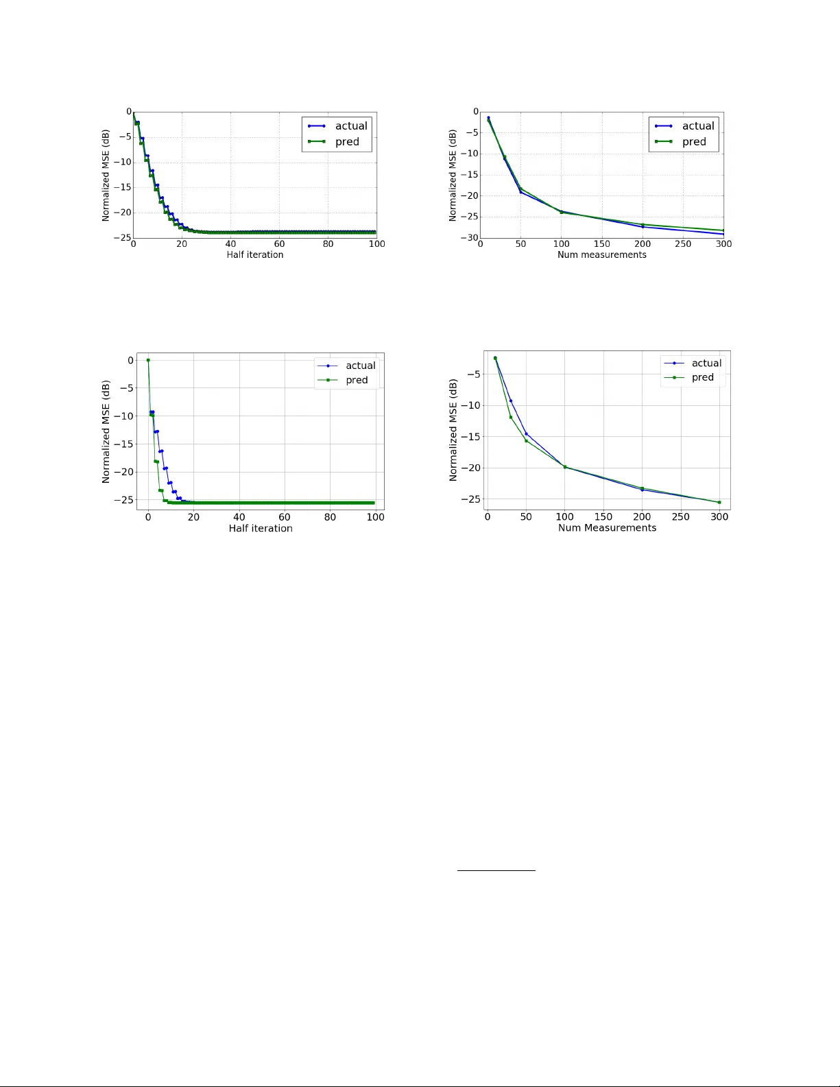
1 Inference with Deep Generati v e Priors in High Dimensions Parthe Pandit, Mojtaba Sahraee-Ardakan, Sundeep Rangan, Philip Schniter , and Alyson K. Fletcher Abstract Deep generativ e priors offer po werful models for complex-structured data, such as images, audio, and text. Using these priors in in verse problems typically requires estimating the input and/or hidden signals in a multi-layer deep neural network from observation of its output. While these approaches have been successful in practice, rigorous performance analysis is complicated by the non-conv ex nature of the underlying optimization problems. This paper presents a no vel algorithm, Multi-Layer V ector Approximate Message Passing (ML-V AMP), for inference in multi-layer stochastic neural networks. ML-V AMP can be conﬁgured to compute maximum a priori (MAP) or approximate minimum mean-squared error (MMSE) estimates for these networks. W e show that the performance of ML-V AMP can be exactly predicted in a certain high-dimensional random limit. Furthermore, under certain conditions, ML-V AMP yields estimates that achiev e the minimum (i.e., Bayes-optimal) MSE as predicted by the replica method. In this way , ML-V AMP provides a computationally efﬁcient method for multi-layer inference with an exact performance characterization and testable conditions for optimality in the large-system limit. P . Pandit, M. Sahraee-Ardakan, and A. K. Fletcher (email: {parthepandit,msahraee,akﬂetcher}@ucla.edu) are with the Departments of Statistics and Electrical and Computer Engineering, the University of California, Los Angeles, CA, 90095. Their work was supported in part by the National Science Foundation under Grants 1254204 and 1738286, and the Ofﬁce of Nav al Research under Grant N00014-15-1-2677. S. Rangan (email: srangan@nyu.edu) is with the Department of Electrical and Computer Engineering, New Y ork Univ ersity , Brooklyn, NY , 11201. His work was supported in part by the National Science Foundation under Grants 1116589, 1302336, and 1547332, as well as the industrial afﬁliates of NYU WIRELESS. P . Schniter (email: schniter .1@osu.edu) is with the Department of Electrical and Computer Engineering, The Ohio State Univ ersity , Columbus, OH, 43210. His work was supported in part by the National Science Foundation under Grant 1716388. Portions of this paper were presented at the IEEE International Symposium on Information Theory in 2018 [1] and 2019 [2]. 2 I . I N T RO D U C T I O N A. Infer ence with Deep Generative Prior s W e consider inference in an L -layer stochastic neural network of the form z 0 ` = W ` z 0 ` − 1 + b ` + ξ ` , ` = 1 , 3 , . . . , L − 1 , (1a) z 0 ` = φ ` ( z 0 ` − 1 , ξ ` ) , ` = 2 , 4 , . . . , L, (1b) where z 0 0 is the network input, { z 0 ` } L − 1 ` =1 are hidden-layer signals, and y := z 0 L is the network output. The odd-index ed layers (1a) are (fully connected) afﬁne linear layers with weights W ` , biases b ` , and additiv e noise vectors ξ ` . The ev en-index ed layers (1b) in volv e separable and possibly nonlinear functions φ ` that are randomized 1 by the noise vectors ξ ` . By “separable, ” we mean that [ φ ` ( z , ξ )] i = φ ` ( z i , ξ i ) ∀ i , where φ ` is some scalar-v alued function, such as a sigmoid or ReLU, and where z i and ξ i represent the i th component of z and ξ . W e assume that the input z 0 0 and noise vectors ξ ` are mutually independent, that each contains i.i.d. entries, and that the number of layers, L , is e ven. A block diagram of the network is shown in the top panel of Fig. 1. The infer ence pr oblem is to estimate the input and hidden signals { z ` } L − 1 ` =0 from an observ ation of the network output y . That is, Estimate { z ` } L − 1 ` =0 gi ven y and { W 2 k − 1 , b 2 k − 1 , φ 2 k } L/ 2 k =1 . (2) For inference, we will assume that network parameters (i.e., the weights W ` , biases b ` , and acti v ation functions φ ` ) are all kno wn, as are the distrib utions of the input z 0 0 and the noise terms ξ ` . Hence, we do not consider the network learning problem. The superscript “ 0 ” on z 0 ` indicates that this is the “true" value of z ` , to be distinguished from the estimates of z ` produced during inference denoted by b z ` . The inference problem (2) arises in the follo wing state-of-the-art approach to in verse problems. In general, solving an “in verse problem" means recov ering some signal x from a measurement y that depends on x . For example, in compressed sensing (CS) [3], the measurements are often 1 The role of the noise ξ `,i in φ ` is allowed to be generic (e.g., additive, multiplicative, etc.). The relationship between z 0 `,i and z 0 ` − 1 ,i will be modeled using the conditional density p ( z 0 `,i | z 0 ` − 1 ,i ) = R δ  z 0 `,i − φ ` ( z 0 ` − 1 ,i , ξ `,i )  p ( ξ `,i ) d ξ `,i . 3 W 1 , b 1 φ 2 ( · ) W 3 , b 3 φ 4 ( · ) z 0 0 z 0 1 z 0 2 z 0 3 y ξ 1 ξ 2 ξ 3 ξ 4 g + 0 ( · ) g ± 1 ( · ) g ± 2 ( · ) g ± 3 ( · ) g − 4 ( · ) y b z + k 0 r + k 0 b z − k 0 r − k 0 b z + k 1 r + k 1 b z − k 1 r − k 1 b z + k 2 r + k 2 b z − k 2 r − k 2 b z + k 3 r + k 3 b z − k 3 r − k 3 Fig. 1. T op panel: Feedfow ard neural network mapping an input z 0 to output y = z 0 4 in the case of L = 4 layers. Bottom panel: ML-V AMP estimation functions g ± ` ( · ) and estimation quantities r ± k` and b z ± k` at iteration k . modeled as y = A x + ξ with known A and additiv e white Gaussian noise (A WGN) ξ , and the signal is often modeled as a sparse linear combination of elements from a known dictionary , i.e., x = Ψz for some sparse coefﬁcient v ector z . T o recover x , one usually computes a sparse coef ﬁcient estimate b z using a LASSO-type con ve x optimization [4] and then uses it to form a signal estimate b x , as in b x = Ψ b z for b z = arg min z  1 2 k y − AΨz k 2 + λ k z k 1  , (3) where λ > 0 is a tunable parameter . The CS recov ery approach (3) can be interpreted as a two-layer version of the inference problem: the ﬁrst layer implements signal generation via x = Ψz , while the second layer implements the measurement process y = Az + ξ . Equation (3) then performs maximum a posteriori inference (see the discussion around (6) ) to recov er estimates of z and x . Although CS has met with some success, it has a limited ability to exploit the complex structure of natural signals, such as images, audio, and video. This is because the model “ x = Ψz with sparse z ” is overly simplistic; it is a one-layer generati ve model. Much more sophisticated modeling is possible with multi-layer priors, as demonstrated in recent works on variational autoencoders (V AEs) [5], [6], generati ve adversarial networks (GANs) [7], [8], and deep image priors (DIP) [9], [10]. These models have had tremendous success in modeling richly structured data, such as images and text. 4 Inference z 0 0 z 0 1 z 0 2 z 0 3 = x 0 b z 3 = b x z 0 4 = y Noise Original Occluded Estimate Generativ e model layers Measurement layer Fig. 2. Moti v ating example: Inference for inpainting [12], [13]. An image x 0 is modeled as the output of a generative model driv en by white noise z 0 0 , and an occluded measurement y is generated by one additional layer . Inference is then used to recover the image x from the measurement y . A typical application of solving an inv erse problem using a deep generativ e model is sho wn in Fig. 2. This ﬁgure considers the classic problem of inpainting [11], for which reconstruction with DIP has been particularly successful [12], [13]. Here, a noise-like signal z 0 0 dri ves a three-layer generati ve network to produce an image x 0 . The generativ e network would hav e been trained on an ensemble of images similar to the one being estimated using, e.g., V AE or GAN techniques. The measurement process, which manifests as occlusion in the inpainting problem, is modeled using one additional layer of the netw ork, which produces the measurement y . Inference is then used to recov er the image x 0 (i.e., the hidden-layer signal z 0 3 ) from y . In addition to inpainting, this deep-reconstruction approach can be applied to other linear in verse problems (e.g., CS, de-blurring, and super-resolution) as well as generalized-linear [14] in verse problems (e.g., classiﬁcation, phase retriev al, and estimation from quantized outputs). W e note that the inference approach pro vides an alternati ve to designing and training a separate reconstruction network, such as in [15]–[17]. When using deterministic deep generati ve models, the unkno wn signal x 0 can be modeled as x 0 = G ( z 0 0 ) , where G is a trained deep neural network and z 0 0 is a realization of an i.i.d. random vector , typically with a Gaussian distribution. Consequently , to recov er x 0 from a linear-A WGN measurement of the form y = A x 0 + ξ , the compressed-sensing approach in (3) can be extended 5 to a regularized least-squares problem [18] of the form b x = G ( b z 0 ) for b z 0 := arg min z 0  1 2 k y − A G ( z 0 ) k 2 + λ k z 0 k 2  . (4) In practice, the optimization in (4) is solved using a gradient-based method. This approach can be straightforwardly implemented with deep-learning software packages and has been used, with excellent results, in [12], [13], [19]–[23]. The minimization (4) has also been useful in interpreting the semantic meaning of hidden signals in deep networks [24], [25]. V AEs [5], [6] and certain GANs [26] can also produce decoding networks that sample from the posterior density , and sampling methods such as Markov-chain Monte Carlo (MCMC) algorithms and Lange vin dif fusion [27], [28] can also be employed. B. Analysis via Appr oximate Message P assing (AMP) While reconstruction with deep generativ e priors has seen tremendous practical success, its performance is not fully understood. Optimization approaches such as (4) are typically non-con vex and difﬁcult to analyze. As we discuss below , most results av ailable today only provide bounds, and these bounds are often be overly conserv ativ e (see Section I-D). Gi ven a network architecture and statistics on the unknown signals, fundamental information- theoretic questions include: What are the precise limits on the accuracy of estimating the hidden signals { z 0 ` } L − 1 ` =0 from the measurements y ? Ho w well do current estimation methods perform relati ve to these limits? Is is possible to design computationally efﬁcient yet optimal methods? T o answer these questions, this paper considers deep inference via approximate message passing (AMP), a po werful approach for analyzing estimation problems in certain high-dimensional random settings. Since its origins in understanding linear in verse problems in compressed sensing [29], [30], AMP has been extended to an impressiv e range of estimation and learning tasks, including generalized linear models [31], models with parametric uncertainty [32], structured priors [33], and bilinear problems [34]. For these problems, AMP-based methods hav e been able to provide computationally efﬁcient algorithms with precise high-dimensional analyses. Often, AMP approaches yield optimality guarantees in cases where all other kno wn approaches do not. 6 C. Main Contributions In this work, we dev elop a multi-layer version of a AMP for inference in deep networks. The proposed approach builds on the recent vector AMP (V AMP) method of [35], which is itself closely related to e xpectation propagation (EP) [36], [37], expectation-consistent approximate inference (EC) [38], [39], S-AMP [40], and orthogonal AMP [41]. The proposed method is called multi-layer V AMP , or ML-V AMP . As will be described in detail below , ML-V AMP estimates the hidden signals in a deep network by cycling through a set of relatively simple estimation functions { g ± ` } L ` =0 . The information ﬂow in ML-V AMP is shown in the bottom panel of Fig. 1. The ML-V AMP method is similar to the multi-layer AMP method of [42] but can handle a more general class of matrices in the linear layers. In addition, as we will describe belo w , the proposed ML-V AMP algorithm can be conﬁgured for either MAP or MMSE estimation. W e will call these approaches MAP-ML-V AMP and MMSE-ML-V AMP . W e establish sev eral ke y results on the ML-V AMP algorithm: • W e show that, for both MAP and MMSE inference, the ﬁx ed points of the ML-V AMP algorithm correspond to stationary points of variational formulations of these estimators. This allo ws the interpretation of ML-V AMP as a Lagrangian algorithm with adaptiv e step-sizes in both cases. These ﬁndings are gi ven in Theorems 1 and 2 and are similar to previous results for AMP [43], [44]. Section III describes these results. • W e prove that, in a certain large system limit (LSL), the behavior of ML-V AMP is exactly described by a deterministic recursion called the state evolution (SE). This SE analysis is a multi-layer e xtension of similar results [35], [45], [46] for AMP and V AMP . The SE equations enable asymptotically exact predictions of macroscopic behaviors of the hidden- layer estimates for each iteration of the ML-V AMP algorithm. This allows us to obtain error bounds e ven if the algorithm is run for a ﬁnite number of iterations. The SE analysis, gi ven in Theorem 3, is the main contribution of the paper , and is discussed in Section IV. • Since the original conference versions of this paper [1], [2], formulae for the minimum mean-squared error (MMSE) for inference in deep networks hav e been conjectured in [47]–[49]. As discussed in Section IV -C , these formulae are based on heuristic techniques, 7 such as the replica method from statistical physics, and hav e been rigorously proven in special cases [50]. Remarkably , we show that the mean-squared-error (MSE) of ML-V AMP exactly matches the predicted MMSE in certain cases. • Using numerical simulations, we verify the predictions of the main result from Theorem 3. In particular , we sho w that the SE accurately predicts the MSE ev en for networks that are not considered large by today’ s standards. W e also perform experiments with the MNIST handwritten digit dataset. Here we consider the inference problem using learned networks, for which the weights do not satisfy the randomness assumptions required in our analysis. In summary , ML-V AMP provides a computationally ef ﬁcient method for inference in deep networks whose performance can be exactly predicted in certain high-dimensional random settings. Moreo ver , in these settings, the MSE performance of ML-V AMP can match the e xisting predictions of the MMSE. D. Prior W ork There has been gro wing interest in studying learning and inference problems in high-dimensional, random settings. One common model is the so-called wide network , where the dimensions of the input, hidden layers, and output are assumed to gro w with a ﬁxed linear scaling, and the weight matrices are modeled as realizations of random matrices. This viewpoint has been taken in [51]–[54], in sev eral works that explicitly use AMP methods [42], [47], [48], [55], and in se veral w orks that use closely related random-matrix techniques [56], [57]. The existing work most closely related to ours is that by Manoel et al. [42], which dev eloped a multi-layer v ersion of the original AMP algorithm [29]. The work [42] provides a state-ev olution analysis of multi-layer inference in networks with entrywise i.i.d. Gaussian weight matrices. In contrast, our results apply to the larger class of rotationally in v ariant matrices (see Section IV for details), which includes i.i.d. Gaussian matrices case as a special case. Se veral other recent works have also attempted to characterize the performance of reconstruction using deep priors in random settings. F or example, when z 0 0 ∈ R k and A ∈ R m × n is a realization of an i.i.d. Gaussian matrix with m = Ω( k L log n ) , Bora et al. [13] showed that an L -layer network 8 G with ReLU activ ations can provide prov ably good reconstruction of x 0 ∈ Range( G ) from measurements y = Ax 0 + ξ . For the same problem, [19] and [58] show that, for W ` ∈ R N ` × N ` − 1 generated entrywise i.i.d. Gaussian and N ` = Ω( N ` − 1 log N ` − 1 ) , one can deriv e bounds on reconstruction error that hold with high probability under similar conditions on m . Furthermore, they also sho w that the cost function of (4) has stationary points in only two disjoint regions of the z 0 space, and both are closely related to the true solution z 0 0 . In [59], the authors use a layer-wise reconstruction scheme to prove reconstruction error bounds when N ` = Ω( N ` − 1 ) , i.e., the network is expansi ve, b ut with a constant factor as opposed to the logarithmic factor in [58]. Our results, in comparison, provide an asymptotically exact characterization of the reconstruction error—not just bounds. Moreover , our results hold for arbitrary hidden-dimension ratios N ` / N ` − 1 , which can be less than, equal to, or greater than one. On the other hand, our results hold only in the large-system limit, whereas the other results abov e hold in the ﬁnite-dimensional regime. Ne vertheless, we think that it should be possible to deriv e a ﬁnite-dimensional v ersion of our analysis (in the spirit of [60]) that holds with high probability . Also, our experimental results suggest that our large-system-limit analysis is a good approximation of behavior at moderate dimensions. Some of the material in this paper appeared in conference versions [1], [2]. The current paper includes all the proofs, simulation details, and pro vides a uniﬁed treatment of both MAP and MMSE estimation. I I . M U L T I - L A Y E R V E C T O R A P P R OX I M A T E M E S S A G E P A S S I N G A. Pr oblem F ormulation W e consider inference in a probabilistic setting where, in (1) , z 0 0 and ξ ` are modeled as random vectors with known densities. Due to the Marko vian structure of { z ` } in (1) , the posterior distribution p ( z | y ) , where z := { z 0 } L − 1 ` =0 , factorizes as p ( z | y ) ∝ p ( z , y ) = p ( z , z L ) = p ( z 0 ) L Y ` =1 p ( z ` | z ` − 1 ) , (5) 9 where the form of p ( z ` | z ` − 1 ) is determined by W ` , b ` , and the distribution of ξ ` for odd ` ; and by φ ` and the distrib ution of ξ ` for e ven ` . W e will assume that z ` ∈ R N ` , where N ` can v ary across the layers ` . Similar to other graphical-model methods [61], we consider two forms of estimation: MAP estimation and MMSE estimation. The maximum a priori , or MAP , estimate is deﬁned as b z map := arg max z p ( z | y ) . (6) Although we will focus on MAP estimation, most of our results will apply to general M -estimators [62] of the form, b z m-est := arg min z ( L 0 ( z 0 ) + L X ` =1 L ` ( z ` , z ` − 1 ) ) for loss functions L ` . The MAP estimator corresponds to the loss function L ` = − ln p ( z ` | z ` − 1 ) . W e will also consider the minimum mean-squared error , or MMSE , estimate, deﬁned as b z mmse := E [ z | y ] = Z z p ( z | y ) d z . (7) T o compute the MMSE estimate, we ﬁrst compute the posterior mar ginals p ( z ` | y ) . W e will also be interested in estimating the posterior marginals p ( z ` | y ) . From estimates of the posterior marginals, one also compute other estimates, such as the mininum mean-absolute error (MMAE) estimate, i.e., the median of the posterior marginal. B. The ML-V AMP Algorithm Similar to the generalized EC (GEC) [39] and generalized V AMP [63] algorithms, the ML- V AMP algorithm attempts to compute MAP or MMSE estimates using a sequence of forward-pass and backward-pass updates. The steps of the algorithm are speciﬁed in Algorithm 1. The quantities updated in the forward pass are denoted by superscript + , and those updated in the backward pass are denoted by superscript − . The update formulae can be deriv ed similarly to those for the GEC algorithm [39], using expectation-consistent approximations of the Gibbs free ener gy inspired by [38]. The ML-V AMP algorithm splits the estimation of z = { z ` } L − 1 ` =1 into smaller 10 Algorithm 1 Multi-layer V ector Approximate Message Passing (ML-V AMP) Require: Estimation functions g + 0 , g − L , and g ± ` for ` = 1 , . . . , L − 1 . 1: Set r − 0 ` = 0 and initialize parameters θ − 0 ` for ` = 0 , 1 , . . . , L − 1 . 2: f or k = 0 , 1 , . . . , N it − 1 do 3: // Forward Pass 4: b z + k 0 = g + 0 ( r − k 0 , θ + k 0 ) 5: α + k 0 =  ∂ g + 0 ( r − k 0 , θ + k 0 ) /∂ r − k`  6: r + k 0 = ( b z + k 0 − α + k 0 r − k 0 ) / (1 − α + k 0 ) 7: f or ` = 1 , . . . , L − 1 do 8: b z + k` = g + ` ( r − k` , r + k,` − 1 , θ + k` ) 9: α + k` =  ∂ g + ` ( r − k` , r + k,` − 1 , θ + k` ) /∂ r − `  10: r + k` = ( b z + k` − α + k` r − k` ) / (1 − α + k` ) 11: end f or 12: 13: // Backward Pass 14: b z − k,L − 1 = g − L ( r + k,L − 1 , θ − kL ) 15: α − k +1 ,L − 1 =  ∂ g − L ( r + k,L − 1 , θ − kL ) /∂ r + k,L − 1  16: r − k + 1 ,L − 1 = ( b z − k,L − 1 − α − k,L − 1 r + k,L − 1 ) / (1 − α − k,L − 1 ) 17: f or ` = L − 1 , . . . , 1 do 18: b z − k,` − 1 = g − ` ( r − k +1 ,` , r + k,` − 1 , θ − k` ) 19: α − k +1 ,` − 1 =  ∂ g − ` ( r − k +1 ,` , r + k,` − 1 , θ − k` ) /∂ r + ` − 1  20: r − k + 1 ,` − 1 = ( b z − k,` − 1 − α − k,` − 1 r + k,` − 1 ) / (1 − α − k,` − 1 ) 21: end f or 22: end f or problems that are solved by the estimation functions { g ± ` } L − 1 ` =1 , g + 0 and g − L . (See Figure 1, bottom panel.) As described below , the form of g ± ` depends on whether the goal is MAP or MMSE estimation. During the forward pass, the estimators g + ` are in voked, whereas in the backward pass, g − ` are in voked. Similarly , the ML-V AMP algorithm maintains two copies, b z + and b z − , of the estimate of z . For ` = 1 , 2 , . . . , L − 1 , each pair of estimators ( g + ` , g − ` ) takes as input r + ` − 1 and r − ` to update the estimates b z + ` and b z − ` − 1 , respecti vely . Similarly , g + 0 and g − L take inputs r − 0 and r + L − 1 to update b z 0 and b z − L − 1 , respectiv ely . The estimation functions also take parameters θ ± ` . 11 C. MAP and MMSE Estimation Functions The form of the estimation functions { g ± ` } L − 1 ` =0 depends on whether the goal is to perform MAP or MMSE estimation. In either case, the parameters are giv en by θ + k 0 = γ − k 0 , θ + k` = ( γ − k` , γ + k,` − 1 ) , θ − k` = ( γ − k +1 ,` , γ + k,` − 1 ) , θ − kL = γ + k,L − 1 , (8) where γ ± k` and η ± k` are scalars updated at iteration k ≥ 0 and all ` = 0 , 1 , . . . , L − 1 as follows: γ + k` = η + k` − γ − k` , γ − k + 1 ,` = η − k +1 ,` − γ + k` , η + k` = γ − k` /α + k` η − k +1 ,` = γ + k` /α − k +1 ,` . (9) Gi ven these parameters, both the MAP and MMSE estimation functions are deﬁned from the belief function b ` ( z ` , z ` − 1 | r − ` , r + ` − 1 , γ − ` , γ + ` − 1 ) ∝ p ( z ` | z ` − 1 ) exp( − γ − ` 2   z ` − r − `   2 − γ + ` − 1 2   z ` − 1 − r + ` − 1   2 ) (10) for ` = 1 , . . . L − 1 . Similarly , b L ( z L , z L − 1 ) ∝ p ( y | z L − 1 ) exp( − γ + L − 1 2 k z L − 1 − r + L − 1 k 2 ) , and b 0 ( z 0 , z − 1 ) ∝ p ( z 0 ) exp( − γ − 0 2 k z 0 − r − 0 k 2 ) . When performing MMSE inference, we use ( b z + ` , b z − ` − 1 ) mmse = g ± `, mmse ( r − ` , r + ` − 1 ; γ − ` , γ + ` − 1 ) = E [( z ` , z ` − 1 ) | b ` ] , (11) where E [ ·| b ` ] denotes expectation with respect to the distribution b ` . Similarly , for MAP inference, we use ( b z + ` , b z − ` − 1 ) map = g ± `, map ( r − ` , r + ` − 1 ; γ − ` , γ + ` − 1 ) = arg max z ` , z ` − 1 b ` ( z ` , z ` − 1 | r − ` , r + ` − 1 , γ − ` , γ + ` − 1 ) . (12) Notice that (12) corresponds to the proximal operator of − ln p ( z ` | z ` − 1 ) . W e will use “MMSE-ML- V AMP” to refer to ML-V AMP with the MMSE estimation functions (11) , and “MAP-ML-V AMP” to refer to ML-V AMP with the MAP estimation functions (12). D. Computational Complexity A key feature of the ML-V AMP algorithm is that, for the neural network (1) , the MMSE and MAP estimation functions (11) and (12) are computationally easy to compute. T o see why , ﬁrst recall that, for the e ven layers ` = 2 , 4 , . . . L , the map φ ` in (1b) is assumed separable and the noise ξ ` is assumed i.i.d. As a result, z ` is conditionally independent giv en z ` − 1 , i.e., 12 p ( z ` | z ` − 1 ) = Q i p ( z `,i | z ` − 1 ,i ) . Thus, for ev en ` , the belief function b ` in (10) also factors into a product of the form b ` ( z ` , z ` − 1 ) = Q i b ` ( z `,i , z ` − 1 ,i ) , implying that the MAP and MMSE versions of g ± ` are both coordinate-wise separable. In other words, the MAP and MMSE estimation functions can be computed using N ` scalar MAP or MMSE estimators. Next consider (1a) for ` = 1 , 3 , . . . , L − 1 , i.e., the linear layers. Assume that ξ ` ∼ N ( 0 , I ν − 1 ` ) for some precision (i.e., in verse v ariance) ν ` > 0 . Then p ( z ` | z ` − 1 ) ∝ ν ` 2 k z ` − W ` z ` − 1 − b ` k 2 . In this case, the MMSE and MAP estimation functions (11) and (12) are identical, and both take the form of a standard least-squares problem. Similar to the V AMP algorithm [35], the least-squares solution—which must be recomputed at each iteration k —is can be efﬁciently computed using a single singular value decomposition (SVD) that is computed once, before the iterations begin. In particular , we compute the SVD W ` = V ` Diag( s ` ) V ` − 1 , (13) where V ` ∈ R N ` × N ` and V ` − 1 ∈ R N ` − 1 × N ` − 1 are orthogonal and Diag( s ` ) ∈ R N ` × N ` − 1 is a diagonal matrix that contains the singular v alues of W ` . Let b ` := V > ` b ` . Then for odd ` , the updates (11) and (12) both correspond to quadratic problems, which can be simpliﬁed by exploiting the rotational in variance of the ` 2 norm. Speciﬁcally , one can deri ve that b z + ` = g + ` ( r − ` , r + ` − 1 , γ − ` , γ + ` − 1 ) = V ` G + ` ( V > ` r − ` , V ` − 1 r + ` − 1 , s ` , b ` , γ − ` , γ + ` − 1 ) (14a) b z − ` − 1 = g − ` ( r − ` , r + ` − 1 , γ − ` , γ + ` − 1 ) = V T ` − 1 G − ` ( V > ` r − ` , V ` − 1 r + ` − 1 , s ` , b ` , γ − ` , γ + ` − 1 ) , (14b) where transformed denoising functions G ± ` ( · ) are componentwise extensions of G ± ` ( · ) , deﬁned as   G + ` ( u ` , u ` − 1 , s ` , b ` , γ − ` , γ + ` − 1 ) G − ` ( u ` , u ` − 1 , s ` , b ` , γ − ` , γ + ` − 1 )   :=   − ν ` s ` γ − ` + ν ` γ + ` − 1 + ν ` s 2 ` − ν ` s `   − 1   γ − ` u ` + ν ` b ` γ + ` − 1 u ` − 1 − ν ` s ` b `   . (15) A detailed deri v ation of equations (14) and (15) is giv en in [64, Appendix B]. Note that the argument s ` in (14a) is N ` dimensional, whereas in (14b) it is N ` − 1 dimensional, i.e., appropriate zero-padding is applied. Keeping this subtlety in mind, we use s ` to keep the notation simple. From Algorithm 1, we see that each pass of the MAP-ML-V AMP or MMSE-ML-V AMP algorithm requires solving (a) scalar MAP or MMSE estimation problems for the non-linear, 13 separable layers; and (b) least-squares problems for the linear layers. In particular, no high- dimensional integrals or high-dimensional optimizations are in volv ed. I I I . F I X E D P O I N T S O F M L - V A M P Our ﬁrst goal is to characterize the ﬁxed points of Algorithm 1. T o this end, let r + ` , r − ` , b z ` with parameters α + ` , α − ` , γ + ` , γ − ` , η ` be a ﬁxed point of the ML-V AMP algorithm, where we hav e dropped the iteration subscript k . At a ﬁx ed point, we do not need to distinguish between b z + ` and b z − ` , nor between η + ` and η − ` , since the updates in (9) imply that η + ` = η − ` = γ + ` + γ − ` =: η ` , α + ` = γ − ` η ` , α − ` = γ + ` η ` , and α + ` + α − ` = 1 . (16) Applying these relationships to lines 10 and 20 of Algorithm 1 giv es b z + ` = b z − ` = γ + ` r + ` + γ − ` r − ` γ + ` + γ − ` =: b z ` . (17) A. F ixed points of MAP-ML-V AMP and connections to ADMM Our ﬁrst results relates the MAP-ML-V AMP updates to an ADMM-type minimization of the MAP objecti ve (6) . For this we use variable splitting , where we replace each variable z ` with two copies, z + ` and z − ` . Then, we deﬁne the objectiv e function F ( z + , z − ) := − ln p ( z + 0 ) − L − 1 X ` =1 ln p ( z + ` | z − ` − 1 ) − ln p ( y | z − L − 1 ) (18) ov er the variable groups z + := { z + ` } L − 1 ` =1 and z − := { z − ` } L − 1 ` =1 . The optimization (6) is then equi v alent to min z + , z − F ( z + , z − ) subject to z + ` = z − ` , ∀ ` = 0 , 1 , . . . , L − 1 . (19) Corresponding to this constrained optimization, we deﬁne the augmented Lagrangian L ( z + , z − , s ) = F ( z + , z − ) + L − 1 X ` =0 η ` s T ` ( z + ` − z − ` ) + L − 1 X ` =0 η ` 2 k z + ` − z − ` k 2 , (20) 14 where s := { s ` } is a set of dual parameters, γ ± ` > 0 are weights, and η ` = γ + ` + γ − ` . No w , for ` = 1 , . . . , L − 2 , deﬁne L ` ( z − ` − 1 , z + ` ; z + ` − 1 , z − ` , s ` − 1 , s ` ) := − ln p ( z + ` | z − ` − 1 ) + η ` s T ` z + ` − η ` − 1 s T ` − 1 z − ` − 1 + γ + ` − 1 2 k z − ` − 1 − z + ` − 1 k 2 + γ − ` 2 k z + ` − z − ` k 2 , (21) which represents the terms in the Lagrangian L ( · ) in (20) that contain z − ` − 1 and z + ` . Similarly , deﬁne L 0 ( · ) and L L − 1 ( · ) using p ( z + 0 ) and p ( y | z + L − 1 ) , respecti vely . One can then verify that L ( z + , z − , s ) = L − 1 X ` =0 L ` ( z − ` − 1 , z + ` ; z + ` − 1 , z − ` , s ` − 1 , s ` ) . Theorem 1 (MAP-ML-V AMP) . Consider the iterates of Algorithm 1 with MAP estimation functions (12) for ﬁxed γ ± ` > 0 . Suppose lines 9 and 19 ar e r eplaced with ﬁxed values α ± k` = α ± ` ∈ (0 , 1) fr om (16) . Let s − k` := α + k` ( b z − k − 1 ,` − r − k` ) and s + k` := α − k` ( r + k` − b z + k` ) . Then, for ` = 0 , . . . , L − 1 , the forwar d pass iterations satisfy , b z + k` = arg min ( z − ` − 1 , z + ` ) L ` ( z − ` − 1 , z + ` ; b z + k,` − 1 , b z − k − 1 ,` , s + k,` − 1 , s − k` ) (22a) s + k` = s − k` + α + ` ( b z + k` − b z − k − 1 ,` ) , (22b) wher eas the backwar d pass iterations satisfy b z − k,` − 1 , = arg min ( z − ` − 1 , z + ` ) L ` ( z − ` − 1 , z + ` ; b z + k,` − 1 , b z − k` , s + k,` − 1 , s − k + 1 ,` ) (23a) s − k + 1 ,` − 1 = s + k,` − 1 + α − ` − 1 ( b z + k,` − 1 − b z − k,` − 1 ) . (23b) Further , any ﬁxed point of Algorithm 1 corr esponds to a critical point of the Lagrangian (20) . Pr oof. See Appendix C  Theorem 1 shows that the ﬁxed- { α ± ` } version of ML-V AMP is an ADMM-type algorithm for solving the optimization problem (19) . In the case that α + ` = α − ` , this algorithm is kno wn as the Peaceman-Rachford Splitting variant of ADMM and its con ver gence has been studied extensi vely; see [65, eqn. (3)] and [66], and the references therein. Different from ADMM, the full ML-V AMP algorithm adaptiv ely updates { α ± k` } in a way that exploits the local curvature 15 of the objectiv e in (12) . Note that, in (22a) and (23a) , we compute the joint minimizers over ( z + ` − 1 , z + ` ) , but only use one of them at a time. B. F ixed P oints of MMSE-ML-V AMP and Connections to F r ee-Ener gy Minimization Recall that z := { z ` } L − 1 ` =0 and let B denote the set of density functions b ( z ) factorizable as f 0 ( z 0 ) f L ( z L − 1 ) Q L − 1 ` =1 f ` ( z ` , z ` − 1 ) . Notice that the true posterior p ( z | y ) from (5) belongs to this set. Essentially , this B captures the chain structure of the factor graph visible in the top panel of Fig. 1. For chain-structured (and, more generally , tree-structured) graphs, one can express any b ∈ B as [67] (see also [68, Sec. III C] for a succinct description) b ( z ) = Q L − 1 ` =1 f ` ( z ` , z ` − 1 ) Q L − 2 ` =1 q ` ( z ` ) , (24) where { f ` ( z ` , z ` − 1 ) } and { q ` ( z ` ) } are marginal density functions of b ( z ) . As marginal densities, they must satisfy the consistent-marginal equations b ( z ` ) = Z f ` ( z ` , z ` − 1 ) d z ` − 1 = q ` ( z ` ) = Z f ` +1 ( z ` +1 , z ` ) d z ` + 1 , ∀ ` = 1 , . . . , L − 1 . (25) Because p ( z | y ) ∈ B , we can express it using v ariational optimization as p ( z | y ) = arg min b ∈B D KL ( b ( z ) k p ( z | y )) , (26) where D KL ( b ( z ) k p ( z | y )) := R b ( z ) ln b ( z ) p ( z | y ) d z is the KL diver gence. Plugging b ( z ) from (24) into (26), we obtain p ( z | y ) = arg min b ∈B ( L X ` =1 D KL ( f ` ( z ` , z ` − 1 ) k p ( z ` | z ` − 1 )) + L − 1 X ` =0 h ( q ` ( z ` )) ) s.t. (25) , (27) where h ( q ` ( z ` )) := − R q ` ( z ` ) ln q ` ( z ` ) d z ` is the differential entropy of q ` . The cost function in (27) is often called the Bethe free ener gy [67]. In summary , because B is tree-structured, Bethe-free-energy minimization yields the exact posterior distrib ution [67]. The constrained minimization (27) is computationally intractable, because both the optimization v ariables { f ` , q ` } and the pointwise linear constraints (25) are inﬁnite dimensional. Rather than solving for the e xact posterior , we might instead settle for an approximation obtained by 16 relaxing the marginal constraints (25) to the following moment-matching conditions, for all ` = 0 , 1 , . . . L − 1 : E [ z ` | f ` ] = E [ z ` | q ` ] , E [ z ` | f ` +1 ] = E [ z ` | q ` ] , E h k z ` k 2    f ` i = E h k z ` k 2    q ` i , E h k z ` k 2    f ` +1 i = E h k z ` k 2    q ` i . (28) This approach is known as expectation-consistent (EC) approximate inference [38]. Because the constraints on f ` and q ` in (28) are ﬁnite dimensional, standard Lagrangian-dual methods can be used to compute the optimal solution. Thus, the EC relaxation of the Bethe free energy minimization problem (27), i.e., min f ` max q ` ( L − 1 X ` =1 D KL ( f ` ( z ` , z ` − 1 ) k p ( z ` | z ` − 1 )) + L − 1 X ` =0 h ( q ` ( z ` )) ) s.t. (28) , (29) yields a tractable approximation to p ( z | y ) . W e now establish an equiv alence between the ﬁxed points of the MMSE-ML-V AMP algorithm and the ﬁrst-order stationary points of (29) . The statement of the theorem uses the belief functions b ` deﬁned in (10). Theorem 2 (MMSE-ML-V AMP) . Consider a ﬁxed point  { r ± ` } , { b z ` } , { γ ± ` }  of Algorithm 1 with MMSE estimation functions (11) . Then { γ + ` r + ` , γ − ` r − ` , γ + ` 2 , γ − ` 2 } , ar e Lagr ange multipliers for (28) such that KKT conditions ar e satisﬁed for the pr oblem (29) at primal solutions { f ∗ ` , q ∗ ` } . Furthermor e, the mar ginal densities take the form f ∗ ` ( · ) ∝ b ` ( ·| r − ` , r + ` − 1 , γ − ` , γ − ` , γ + ` − 1 ) and q ∗ ` = N ( b z ` , I /η ` ) , with b z ` and η ` given in (16) - (17) . Pr oof. See Appendix C.  The abov e result shows that MMSE-ML-V AMP is essentially an algorithm to iterati vely solv e for the parameters  { r ± ` } , { b z ` } , { γ ± ` }  that characterize the EC ﬁxed points. Importantly , q ∗ ` ( z ` ) and f ∗ ( z ` , z ` − 1 ) serve as an approximate marginal posteriors for z ` and ( z ` , z ` − 1 ) . This enables us to not only compute the MMSE estimate (i.e., posterior mean), but also other estimates like the MMAE estimate (i.e., the posterior median), or quantiles of the marginal posteriors. Remarkably , in certain cases, these approximate marginal-posterior statistics become exact. This is one of the main contributions of the next section. 17 I V . A N A L Y S I S I N T H E L A R G E - S Y S T E M L I M I T A. LSL model In the previous section, we established that, for any set of deterministic matrices { W ` } , MAP-ML-V AMP solves the MAP problem and MMSE-ML-V AMP solves the EC variational inference problem as the iterations k → ∞ . In this section, we extend the analysis of [35], [45] to the rigorously study the behavior of ML-V AMP at any iteration k for classes of random matrices { W ` } in a certain large-system limit (LSL). The model is described in the follo wing set of assumptions. System model: W e consider a sequence of systems index ed by N . For each N , let z ` = z 0 ` ( N ) ∈ R N ` ( N ) be “true” vectors generated by neural network (1) for layers ` = 0 , . . . , L , such that layer widths satisfy lim N →∞ N ` ( N ) / N = β ` ∈ (0 , ∞ ) . Also, let the weight matrices W ` in (1a) each have an SVD gi ven by (13) , where { V ` } are drawn uniformly from the set of orthogonal matrices in R N ` × N ` and independent across ` . The distribution on the singular v alues s ` will be described below . Similar to the V AMP analysis [35], the assumption here is that weight matrices W ` are rotationally in variant, meaning that VW ` and W ` V are distributed identically to W ` . Gaussian i.i.d. W ` as considered in the original ML-AMP work of [42] satisfy this rotationally in v ariant assumption, b ut the rotationally in variant model is more general. In particular , as described in [35], the model can hav e arbitrary coniditoning which is kno wn to be a major failure mechanism of AMP methods. ML-V AMP algorithm: W e assume that we generate estimates b z ± k` from the ML-V AMP algorithm, Algorithm 1. Our analysis will apply to general estimation functions, g ` ( · ) , not necessarily the MAP or MMSE estimators. Ho wever , we require tw o technical conditions: For the non-linear estimators, g ± ` for ` = 2 , 4 , . . . L − 2 , and g + 0 , g − L act componentwise. Further , these estimators and their deriv atives g + ` ∂ z − ` , g − ` ∂ z + ` − 1 , g + 0 ∂ z − 0 , g − L ∂ z + L − 1 are uniformly Lipschitz continuous. The technical deﬁnition of uniformly Lipschitz continuous is giv en in Appendix A. For the linear layers, ` = 1 , 3 , . . . L − 1 , we assume we apply estimators g ± ` of the form (14) where G ± ` act componentwise. Further , G ± ` along with its deri vati ves are uniformly Lipschitz continuous. 18 W e also assume that the activ ation functions φ ` in equation (1b) are componentwise separable and Lipschitz continuous. T o simplify the analysis, we will also assume the estimation function parameters θ ± k` con ver ge to ﬁxed limits, lim N →∞ θ ± k` ( N ) = θ ± k` , (30) for values θ ± k` . Importantly , in this assumption, we assume that the limiting parameter values θ ± k` are ﬁxed and not data dependent. Ho we ver , data dependent parameters can also be modeled [35]. Distribution of the components: W e follow the framew ork of Bayati-Montanari and describe the statistics on the unknown quantities via their empirical conv ergence – see Appendix A. For ` = 1 , 3 , . . . L − 1 , deﬁne b ` := V T ` b ` and ξ ` := V T ` ξ ` . W e assume that the sequence of true vectors z 0 0 , singular values s ` , bias vectors b ` , and noise realizations ξ ` empirically con verge as lim N →∞  z 0 0 ,n  P L (2) = Z 0 0 , lim N →∞ { ξ `,n } P L (2) = Ξ ` , ` = 2 , 4 , . . . , L (31a) lim N →∞  ( s `,n , b `,n , ξ `,n )  P L (2) = ( S ` , B ` , Ξ ` ) , ` = 1 , 3 , . . . , L − 1 , (31b) to random variables Z 0 0 , Ξ ` , S ` , B ` , Ξ ` . W e will also assume that the singular values are bounded, i.e., s `,n < S `, max ∀ n . Also, the initial vectors r − 0 ` con ver ge as, lim N →∞  [ r − 0 ` − z 0 ` ] n  P L (2) = Q − 0 ` , ` = 0 , 2 , . . . , L,  [ V > ` ( r − 0 ` − z 0 ` )] n  P L (2) = Q − 0 ` , ` = 1 , 3 , . . . , L − 1 , (32) where ( Q − 0 ` , Q − 1 ` , . . . Q − L − 1 ,` ) is jointly Gaussian independent of Z 0 0 , { Ξ ` } , { S ` , B ` , Ξ ` } . State Evolution: Under the abov e assumptions, our main result is to sho w that the asymptotic distribution of the quantities from ML-V AMP algorithm con ver ge to certain distrib utions. The distributions are described by a set of deterministic parameters { K + k` , τ − k` , α ± k` , γ ± k` , η ± k` } . The e volv e according to a scalar recursion called the state ev olution (SE), giv en in Algorithm 2 in Appendix B. W e assume α ± k` ∈ (0 , 1) for all iterations k and ` = 0 , 1 , . . . L − 1 . B. SE Analysis in the LSL Under these assumptions, we can now state our main result. 19 Theorem 3. Consider the system under the above assumptions. F or any componentwise pseudo- Lipschitz function ψ of or der 2, iteration inde x k , and layer index ` = 2 , 4 , . . . L − 2 , lim N →∞ D ψ  z 0 ` − 1 , b z − k,` − 1 , b z + k`  E a.s. − − → E  ψ  A , g − ` ( C + A , B + A , γ − k` , γ + k,` − 1 ) , g + ` ( C + A , B + A , γ − k` , γ + k,` − 1 )  , (33) lim N →∞  ψ ( z , 0 0 b z + k 0 )  a.s. − − → E  ψ ( g + 0 ( C 0 + Z 0 0 ) , γ − 0 )  , (34) lim N →∞  ψ ( z 0 L − 1 , b z − k,L − 1 )  a.s. − − → E  ψ ( A 0 , g − L ( B 0 + A 0 , γ + L − 1 ))  , (35) wher e ( A , B ) ∼ N (0 , K + k` ) and C ∼ N (0 , τ − k` ) ar e mutually independent and independent of Ξ ` ; ( A 0 , B 0 ) ∼ N (0 , K + kL ) is independent of Ξ L and C 0 ∼ N (0 , τ − k 0 ) is independent of Z 0 0 . Similarly for any layer index ` = 1 , 3 , . . . , L − 1 , we have lim N →∞  ψ  V ` − 1 z 0 ` − 1 , V ` − 1 b z − k,` − 1 , V > ` b z + k`  a.s. − − → E  ψ  A , G − ` ( C + A , B + A , S ` , B ` , γ − k` , γ + k,` − 1 ) , G + ` ( C + A , B + A , S ` , B ` , γ − k` , γ + k,` − 1 )  , (36) wher e ( A , B ) ∼ N (0 , K + k` ) and C ∼ N (0 , τ − k` ) ar e mutually independent and independent of ( S ` , B ` , Ξ ` ) . Furthermor e, if γ ± k` , η ± k` , ar e deﬁned analogous to (9) using α ± k` , then for all ` , lim N →∞ ( α ± k,` , γ ± k,` , η ± k,` ) a.s. − − → ( α ± k,` , γ ± k,` , η ± k,` ) . (37) Pr oof. See Appendix F.  The ke y v alue of Theorem 3 is that we can exactly char acterize the asymptotic joint distribution of the true vectors z 0 ` and the ML-V AMP estimates b z ± k` . The asymptotic joint distribution, can be used to compute v arious key quantities. For e xample, suppose we wish to compute the mean squared error (MSE). Let ψ ( z 0 , b z ) = ( z 0 − b z ) 2 , whereby  ψ ( z 0 ` , b z − ` )  = 1 N   z 0 ` − b z − `   2 . Observe that ψ is a pseudo-Lipschitz function of order 2, whereby we can apply Theorem 3. Using (33) , we get the asymptotic MSE on the k th -iteration estimates for ` = 2 , 4 , . . . L − 2 : lim N ` − 1 →∞ 1 N ` − 1   b z − k,` − 1 − z 0 ` − 1   2 a.s. − − → E h  g − ` ( C + A , B + A , γ − k` , γ + k,` − 1 ) − A  2 i , lim N ` →∞ 1 N `   b z + k` − z 0 `   2 a.s. − − → E h  g + ` ( C + A , B + A , γ − k` , γ + k,` − 1 ) − φ ` ( A , Ξ ` )  2 i , 20 where we used the fact that φ ` is pseudo-Lipschitz of order 2, and z 0 ` = φ ` ( z 0 ` − 1 , ξ ` ) from (1b) . Similarly , using (36), we get the k th-iteration MSE for ` = 1 , 3 , . . . L − 1 : lim N ` − 1 →∞ 1 N ` − 1   b z − k,` − 1 − z 0 ` − 1   2 = lim N ` − 1 →∞ 1 N ` − 1   V ` − 1 ( b z − k,` − 1 − z 0 ` − 1 )   2 a.s. − − → E h  G − ` ( C + A , B + A , S ` , B ` , γ + k,l , γ − k,` − 1 ) − A  2 i . lim N ` →∞ 1 N `   b z + k` − z 0 `   2 = lim N ` →∞ 1 N `   V > ` ( b z + k` − z 0 ` )   2 a.s. − − → E h  G + ` ( C + A , B + A , γ + kl , γ − k,` − 1 ) − S ` A − B `  2 i , where we used the rotational in variance of the ` 2 norm, and the fact that equation (1a) is equiv alent to V > ` z 0 ` = Diag( s ` ) V ` − 1 z 0 ` − 1 + b ` using the SVD (13) of the weight matrices W ` . At the heart of the proof lies a key insight: Due to the randomness of the unitary matrices V ` , the quantities ( z 0 ` , r − k` − z 0 ` , r + k,` − 1 − z 0 ` − 1 ) are asymptotically jointly Gaussian for e ven ` , with the asymptotic cov ariance matrix of { ( z 0 ` − 1 ,n , r + k,` − 1 ,n − z 0 ` − 1 ,n , r − k`,n − z 0 `,n ) } gi ven by h K + k` 0 0 τ − k` i , where K k` ∈ R 2 × 2 and τ − k` is a scalar . After establishing the asymptotic Gaussianity of ( z 0 ` , r − k` − z 0 ` , r + k,` − 1 − z 0 ` − 1 ) , since b z ` and b z ` − 1 are componentwise functions of this triplet, we have the PL(2) con ver gence result in (33) . Similarly , for odd ` , we can show that  V ` − 1 z 0 ` − 1 , V ` − 1 r + k,` − 1 , V > ` r − k`  is asymptotically Gaussian. For these ` , V ` − 1 b z − k,` − 1 and V > ` b z + k` are functions of the triplet, which gi ves the result in (36). Due to the asymptotic normality mentioned abov e, the inputs ( r − ` , r + ` − 1 ) to the estimators g ± ` are the true signals ( z 0 ` − 1 , z 0 ` ) plus additi ve white Gaussian noise (A WGN). Hence, the estimators g ± ` act as denoisers, and ML-V AMP effecti vely reduces the inference problem 2 into a sequence of linear transformations and denoising problems. The denoising problems are solved by g ± ` for e ven ` , and by G ± ` for odd ` . C. MMSE Estimation and Connections to the Replica Pr edictions W e next consider the special case of using MMSE estimators corresponding to the true distributions. In this case, the SE equations simplify considerably using the following MSE functions : let b z − ` − 1 , b z + ` be the MMSE estimates of z 0 ` − 1 and z 0 ` from the variables r + ` − 1 , r − ` under 21 the joint density (10). Let E ± ( · ) be the corresponding mean squared errors, E + ` ( γ + ` − 1 , γ − ` ) := lim N →∞ 1 N E   z 0 ` − b z + `   2 , E − ` − 1 ( γ + ` − 1 , γ − ` ) := lim N →∞ 1 N E   z 0 ` − 1 − b z − ` − 1   2 . (38) Theorem 4 (MSE of MMSE-ML-V AMP) . Consider the system under the assumptions of Theor em 3, with MMSE estimation functions g ± ` , g + 0 , g − L fr om (11) for the belief estimates in (10) with γ + k` = γ ± k` fr om the state-evolution equations. Then, the state evolution equations r educe to γ + k` = 1 E + ` ( γ − k` , γ + k,` − 1 ) − γ − k` , γ − k +1 ,` = 1 E − ` ( γ − k +1 ,` +1 , γ + k` ) − γ + k` , (39) wher e 1 /η + k` = E + ` ( γ − k` , γ + k,` − 1 ) is the MSE of the estimate b z + k` . Pr oof. See Appendix F.  Since the estimation functions in Theorem 4 are the MSE optimal functions for true densities, we will call this selection of estimation functions the MMSE matched estimators . Under the assumption of MMSE matched estimators, the theorem shows that the MSE error has a simple set of recursiv e expressions. It is useful to compare the predicted MSE with the predicted optimal values. The works [47], [48] postulate the optimal MSE for inference in deep networks under the LSL model described abov e using the replica method from statistical physics. Interestingly , it is sho wn in [47, Thm.2] that the predicted minimum MSE satisﬁes equations that exactly agree with the ﬁxed points of the updates (39) . Thus, when the ﬁxed points of (39) are unique, ML-V AMP with matched MMSE estimators prov ably achiev es the Bayes optimal MSE predicted by the replica method. Although the replica method is not rigorous, this MSE predictions hav e been indepedently prov en for the Gaussian case in [47] and certain two layer networks in [48]. This situation is similar to sev eral other works relating the MSE of AMP with replica predictions [50], [69]. The consequence is that, if the replica method is correct, ML-V AMP provides a computationally efﬁcient method for inference with testable conditions under which it achie ves the Bayes optimal MSE. 22 V . N U M E R I C A L S I M U L A T I O N S W e no w numerically in vestigate the MAP-ML-V AMP and MMSE-ML-V AMP algorithms using two sets of experiments, where in each case the goal was to solve an estimation problem of the form in (2) using a neural network of the form in (1). W e used the Python 3.7 implementation of the ML-V AMP algorithm av ailable on GitHub . 2 The ﬁrst set of experiments uses random draws of a synthetic network to v alidate the claims made about the ML-V AMP state-e volution (SE) in Theorem 3. In addition, it compares MAP- ML-V AMP and MMSE-ML-V AMP to the MAP approach (4) using a standard gradient-based solver , AD AM [70]. The second set of e xperiments applies ML-V AMP to image inpainting, using images of handwritten digits from the widely used MNIST dataset. There, MAP-ML-V AMP and MSE-ML-V AMP were compared to Stochastic Gradient Lange vin Dynamics (SGLD) [28], an MCMC-based sampling method that approximates E [ z | y ] , as well as to the optimization approach (4) using the AD AM solver . A. P erformance on a Synthetic Network W e ﬁrst considered a 7-layer neural network of the form in (1) . The ﬁrst six layers, with dimensions N 0 = 20 , N 1 = N 2 = 100 , N 3 = N 4 = 500 , N 5 = N 6 = 784 , formed a (deterministic) deep generativ e prior driv en by i.i.d. Gaussian z 0 0 . The matrices W 1 , W 3 , W 5 and biases b 1 , b 3 , b 5 were drawn i.i.d. Gaussian, and the activ ation functions φ 2 , φ 4 , φ 6 were ReLU. The mean of the bias vectors b ` was chosen so that a ﬁxed fraction, ρ , of the linear outputs were positiv e, so that only the fraction ρ of the ReLU outputs were non-zero. Because this generati ve network is random rather than trained, we refer to it as “synthetic. ” The ﬁnal layer , which takes the form y = Az 0 6 + ξ 6 , generates noisy , compressed measurements of z 0 6 . Similar to [71], the matrix A ∈ R M × N 6 was constructed from the SVD A = U Diag ( s ) V T , where the singular- vector matrices U and V were drawn uniformly from the set of orthogonal matrices, and the singular v alues were geometrically spaced (i.e., s i /s i − 1 = κ ∀ i ) to achiev e a condition number of s 1 /s M = 10 . It is known that such matrices cause standard AMP algorithms to fail [71], but 2 See https://github .com/GAMPT eam/vampyre. 23 Fig. 3. NMSE of MMSE-ML-V AMP and its SE prediction when estimating the input to a randomly generated 7-layer neural network (see text of Section V -A ). Left panel: A verage NMSE versus half-iteration with M = 100 measurements. Right panel: A verage NMSE verus measurements M at after 50 iterations. Fig. 4. Simulation with randomly generated neural network with MAP estimators from equation (12) . Left panel: Normalized mean squared error (NMSE) for ML-V AMP and the predicted MSE as a function of the iteration with M = 100 measurements. Right panel: Final NMSE (50 iterations) for ML-V AMP and the predicted MSE as a function of the number of measurements, M . ρ = 0 . 9 not V AMP algorithms [35]. The number of compressed measurements, M , was varied from 10 to 300, and the noise vector ξ was drawn i.i.d. Gaussian with a variance set to achiev e a signal-to-noise ratio of 10 log 10 ( E k A z 0 6 k 2 / E k ξ k 2 ) = 30 dB. T o quantify the performance of ML-V AMP , we repeated the follo wing 1000 times. First, we dre w a random neural network as described abov e. Then we ran the ML-V AMP algorithm for 100 iterations, recording the normalized MSE (in dB) of the iteration- k estimate of the network input, b z ± k 0 : NMSE( b z ± k 0 ) := 10 log 10  k z 0 0 − b z ± k 0 k 2 k z 0 0 k 2  . Since ML-V AMP computes two estimates of z 0 0 at each iteration, we consider each estimate as corresponding to a “half iteration. ” 24 Fig. 5. Simulation with randomly generated neural network with MAP estimators from equation (12) . Final NMSE for (a) MAP inference computed by Adam optimizer; (b) MAP inference from ML-V AMP; (c) State evolution prediction. a) V alidation of SE Pr ediction: For MMSE-ML-V AMP , the left panel of Fig. 3 shows the NMSE versus half-iteration for M = 100 compressed measurements. The value shown is the av erage ov er 1000 random realizations. Also shown is the MSE predicted by the ML-V AMP state ev olution. Comparing the two traces, we see that the SE predicts the actual behavior of MMSE-ML-V AMP remarkably well, within approximately 1 dB. The right panel sho ws the NMSE after k = 50 iterations (i.e., 100 half-iterations) for se veral numbers of measurements M . Again we see an excellent agreement between the actual MSE and the SE prediction. In both cases we used the positiv e fraction ρ = 0 . 4 . Analogous results are shown for MAP-ML-V AMP in Fig. 4. There we see an excellent agreement between the actual MSE and the SE prediction for iterations k ≥ 15 and all values of M . b) Comparison to AD AM: W e now compare the MSE of MAP-ML-V AMP and its SE to that the MAP approach (4) using the AD AM optimizer [70], as implemented in T ensorﬂow . As before, the goal was to recov er the input z 0 0 to the 7-layer synthetic network from a measurement of its output. Fig. 5 shows the median NMSE ov er 40 random network realizations for sev eral values of M , the number of measurements. W e see that, for M ≥ 100 , the performance of MAP-ML-V AMP closely matches its SE prediction, as well as the performance of the AD AM-based MAP approach (4) . For M < 100 , there is a discrepancy between the MSE performance of MAP-ML-V AMP and its SE prediction, which is likely due to the relativ ely small dimensions in volv ed. Also, 25 for small M , MAP-ML-V AMP appears to achiev e slightly better MSE performance than the AD AMP-based MAP approach (4) . Since both are attempting to solve the same problem, the dif ference is likely due to ML-V AMP ﬁnding better local minima. B. Image Inpainting: MNIST dataset T o demonstrate that ML-V AMP can also work on a real-world dataset, we perform inpainting on the MNIST dataset. The MNIST dataset consists of 28 × 28 = 784 pixel images of handwritten digits, as shown in the ﬁrst column of Fig. 6. T o start, we trained a 4-layer (deterministic) deep generativ e prior model from 50 000 digits using a variational autoencoder (V AE) [6]. The V AE “decoder” network was designed to accept 20-dimensional i.i.d. Gaussian random inputs z 0 with zero mean and unit variance, and to produce MNIST -like images x . In particular , this network began with a linear layer with 400 outputs, follo wed by a ReLU activ ations, followed by a linear layer with 784 units, followed by sigmoid acti v ations that forced the ﬁnal pixel v alues to between 0 and 1. Gi ven an image, x , our measurement process produced y by erasing rows 10-20 of x , as sho wn in the second column of Fig. 6. This process is known as “occlusion. ” By appending the occlusion layer onto our deep generati ve prior , we got a 5-layer network that generates an occluded MNIST image y from a random input z 0 . The “inpainting problem” is to recover the image x = z 4 from the occluded image y . For this inpainting problem, we compared MAP-ML-V AMP and MMSE-ML-V AMP to the MAP estimation approach (4) using the AD AM solver , and to Stochastic Gradient Langevin Dynamics (SGLD) [28], an MCMC-based sampling method that approximates E [ z | y ] . Example image reconstructions are shown in Fig. 6. There we see that the qualitative performance of ML-V AMP is comparable to the baseline solvers. V I . C O N C L U S I O N Inference using deep generati ve prior models provides a powerful tool for complex in verse problems. Rigorous theoretical analysis of these methods has been difﬁcult due to the non-con ve x nature of the models. The ML-V AMP methodology for MMSE as well as MAP estimation 26 Fig. 6. MNIST inpainting: Original 28 × 28 images of handwritten digits (Col 1), with ro ws 10-20 are erased (Col 2). Comparison of reconstructions using MAP estimation with ADAM solver (Col 3), MAP estimation with ML-V AMP algorithm (Col 4), MMSE estimation with the SGLD approach (Col 5), and MMSE estimation with ML-V AMP algorithm (Col 6). provides a principled and computationally tractable method for performing the inference whose performance can be rigorously and precisely characterized in a certain large system limit. The approach thus offers a ne w and potentially powerful approach for understanding and improving deep neural network based models for inference. A P P E N D I X A E M P I R I C A L C O N V E R G E N C E O F V E C T O R S E Q U E N C E S W e follo w the framework of Bayati and Montanari [45], which models v arious sequences as deterministic, but with components con ver ging empirically to a distribution. W e start with a brief revie w of useful deﬁnitions. Let x ( N ) = ( x 1 , . . . , x N ) be a block vector with components x n ∈ R r for some r . Thus, the vector x ( N ) is a vector with dimension r N . Giv en any function g : R r → R s , we deﬁne the componentwise extension of g ( · ) as the function, g ( x ) := ( g ( x 1 ) , . . . , g ( x N )) ∈ R N s . (40) 27 That is, g ( · ) applies the function g ( · ) on each r -dimensional component. Similarly , we say g ( x ) acts componentwise on x whenev er it is of the form (40) for some function g ( · ) . Next consider a sequence of block vectors of gro wing dimension, x ( N ) = ( x 1 ( N ) , . . . , x N ( N )) , N = 1 , 2 , . . . , where each component x n ( N ) ∈ R r . In this case, we will say that x ( N ) is a block vector sequence that scales with N under blocks x n ( N ) ∈ R r . When r = 1 , so that the blocks are scalar , we will simply say that x ( N ) is a vector sequence that scales with N . Such vector sequences can be deterministic or random. In most cases, we will omit the notational dependence on N and simply write x . No w , giv en p ≥ 1 , a function f : R r → R s is called pseudo-Lipsc hitz continuous of order p , if there exists a constant C > 0 such that for all x 1 , x 2 ∈ R r , k f ( x 1 ) − f ( x 2 ) k ≤ C k x 1 − x 2 k  1 + k x 1 k p − 1 + k x 2 k p − 1  . Observe that in the case p = 1 , pseudo-Lipschitz continuity reduces to usual Lipschitz continuity . Gi ven p ≥ 1 , we will say that the block vector sequence x = x ( N ) con ver ges empirically with p -th or der moments if there exists a random v ariable X ∈ R r such that (i) E k X k p p < ∞ ; and (ii) for any f : R r → R that is pseudo-Lipschitz continuous of order p , lim N →∞ 1 N N X n =1 f ( x n ( N )) = E [ f ( X )] . (41) In (41) , we hav e the empirical mean of the components f ( x n ( N )) of the componentwise extension f ( x ( N )) con ver ging to the expectation E [ f ( X )] . In this case, with some abuse of notation, we will write lim N →∞ { x n } P L ( p ) = X , (42) where, as usual, we have omitted the dependence on N in x n ( N ) . Importantly , empirical con ver gence can be deﬁned on deterministic v ector sequences, with no need for a probability space. If x = x ( N ) is a random vector sequence, we will often require that the limit (42) holds 28 almost surely . Finally , we introduce the concept of uniform pseduo-Lipschitz continuity . Let φ ( r , γ ) be a function on r ∈ R r and θ ∈ R s . W e say that φ ( r , θ ) is uniformly Lipschitz continuous in r at θ = θ if there exists constants L 1 , L 2 ≥ 0 and an open neighborhood U of θ such that k φ ( r 1 , θ ) − φ ( r 2 , θ ) k ≤ L 1 k r 1 − r 2 k , ∀ r 1 , r 2 ∈ R r , θ ∈ U (43a) k φ ( r , θ 1 ) − φ ( r , θ 2 ) k ≤ L 2 (1 + k r k ) k θ 1 − θ 2 k , ∀ r ∈ R r , θ 1 , θ 2 ∈ U. (43b) A P P E N D I X B M L - V A M P S TA T E E V O L U T I O N E Q UA T I O N S The state ev olution (SE) recursiv ely deﬁnes a set of scalar random variables that describe the typical components of the vector quantities produced from the ML-V AMP algorithm. The deﬁnition of the random variables are giv en in Algorithm 2. The algorithm steps mimic those in the ML-V AMP algorithm, Algorithm 1, but with each update producing scalar random variables instead of vectors. The updates use se veral functions: f 0 0 ( w 0 ) = w 0 , f 0 ` ( p 0 ` − 1 , w ` ) := f 0 ` ( p 0 ` − 1 , ξ ` ) := φ ` ( p 0 ` − 1 , ξ ` ) , ` = 2 , 4 , . . . , L, (44a) f 0 ` ( p 0 ` − 1 , w ` ) := f 0 ` ( p 0 ` − 1 , ( ¯ s ` , ¯ b ` , ¯ ξ ` )) = ¯ s ` p 0 ` − 1 + ¯ b ` + ¯ ξ ` , ` = 1 , 3 , . . . , L − 1 , (44b) h ± ` ( p 0 ` − 1 , p + ` − 1 , q − ` , w ` , θ ± k` ) = g ± ` ( q − ` + q 0 ` , p + ` − 1 + p 0 ` − 1 , θ ± k` ) , ` = 2 , 4 , . . . L − 2 , (44c) h ± ` ( p 0 ` − 1 , p + ` − 1 , q − ` , w ` , θ ± k` ) = G ± ` ( q − ` + q 0 ` , p + ` − 1 + p 0 ` − 1 , θ ± k` ) , ` = 1 , 3 , . . . L − 1 , (44d) h + 0 ( q − 0 , w 0 θ + k 0 ) = g + 0 ( q − 0 + w 0 , θ + k 0 ) , h − L ( p 0 L − 1 , p + L − 1 , w L , θ − kL ) = g − L ( p + L − 1 + p 0 L − 1 , θ − kL ) , (44e) f + 0 ( q − 0 , w 0 , Λ + k 0 ) := 1 1 − α + k`  h + 0 ( q − 0 , w 0 , θ + k 0 ) − w 0 − α + k 0 q − 0  , (44f) f + ` ( p 0 ` − 1 , p + ` − 1 , q − ` , w ` , Λ + k` ) := 1 1 − α + k`  h + ` ( p 0 ` − 1 , p + ` − 1 , q − ` , w ` , θ + k` ) − q 0 ` − α + k` q − `  , (44g) f − L ( p 0 L − 1 , p + L − 1 , w L , Λ − kL ) := 1 1 − α − k`  h − L ( p 0 L − 1 , p + L − 1 , w L , θ − kL ) − p 0 L − 1 − α − k,L − 1 p + L − 1  , (44h) f − ` ( p 0 ` − 1 , p + ` − 1 , q − ` , w ` , Λ − k` ) := 1 1 − α − k,` − 1  h − ` ( p 0 ` − 1 , p + ` − 1 , q − ` , w ` , θ − k` ) − p 0 ` − 1 − α − k,` − 1 p + ` − 1  . (44i) 29 In addition deﬁne the perturbation random variables W ` (recall from (31)) as W 0 = Z 0 0 , W ` = Ξ ` , ` = 2 , 4 , . . . , L − 2 , (45a) W ` = ( S ` , B ` , Ξ ` ) , ` = 1 , 3 , . . . , L − 1 . (45b) A P P E N D I X C P RO O F S O F M L - V A M P F I X E D - P O I N T T H E O R E M S A. Pr oof of Theor em 1 The linear equalities in deﬁning s ± k` can be rewritten as, r + k` = b z + k` + 1 α − k` s + k` , r − k +1 ,` = b z − k` − 1 α + k` s − k + 1 ,` (46) Substituting (46) in lines 10 and 20 of Algorithm 1 gi ve the updates (22b) and (23b) in Theorem 1. It remains to show that the optimization problem in updates (22a) and (23a) is equi v alent to (12) . It sufﬁ ces to show that the terms dependent on ( z − ` − 1 , z + ` ) in b ` from (12) , and L ` from (22a) and (23a) are identical. This follows immediately on substituting (46) in (10) . Thus there exists a bijecti ve mapping between the ﬁxed points { b z , r + , r − } (of Algorithm 1) and { b z , s } (of Theorem 1). It now remains to be shown that an y ﬁxed point of Algorithm 1 is a critical point of the augmented Lagrangian in (20) . T o that end, we need to sho w that there e xists dual parameters s ` such that for all ` = 0 , . . . , L − 1 , b z + ` = b z − ` , ∂ z + L ( b z + , b z − , s ) 3 0 , ∂ z − L ( b z + , b z − , s ) 3 0 , (47) where L ( · ) is the Lagrangian in (20) . Primal feasibility or b z + ` = b z − ` was already sho wn in (17) . As a consequence of the primal feasibility b z + ` = b z − ` , observe that s + ` − s − ` = ( α + ` + α − ` ) b z ` − α + ` r − ` − α − ` r + ` = 0 , (48) where we have used (16) . Deﬁne s := s + = s − . T o show the stationarity in (47) it sufﬁces to 30 Algorithm 2 State Evolution for ML-V AMP Require: f 0 ` ( · ) , f ± ` ( · ) and h ± ` ( · ) from eqn. (44) and initial random variables: Z 0 0 , { W ` , Q − 0 ` } from Section IV and (45) 1: // Initial pass 2: Q 0 0 = Z 0 0 , τ 0 0 = E ( Q 0 0 ) 2 and P 0 0 ∼ N (0 , τ 0 0 ) 3: f or ` = 1 , . . . , L − 1 do 4: Q 0 ` = f 0 ` ( P 0 ` − 1 , W ` ) 5: P 0 ` ∼ N (0 , τ 0 ` ) , τ 0 ` = E ( Q 0 ` ) 2 6: end f or 7: 8: f or k = 0 , 1 , . . . do 9: // Forward Pass 10: b Q + k 0 = h + 0 ( Q − k 0 , W 0 , θ + k 0 )) 11: α + k 0 = E ( ∂ h + 0 ∂ Q − k 0 ( Q − k 0 , W 0 , θ + k 0 )) , Λ + k 0 = ( α + k 0 , θ + k 0 ) 12: Q + k 0 = f + 0 ( Q − 0 , W 0 , Λ + k 0 ) 13: ( P 0 0 , P + k 0 ) ∼ N ( 0 , K + k 0 ) , K + k 0 := Co v( Q 0 0 , Q + k 0 ) 14: f or ` = 1 , . . . , L − 1 do 15: b Q + k` = h + ` ( P 0 ` − 1 , P + k,` − 1 , Q − k` , W ` , θ + k` )) 16: α + k` = E ( ∂ h + ` ∂ Q − k` ( P 0 ` − 1 , P + k,` − 1 , Q − k` , W ` , θ + k` )) , Λ + k` = ( α + k` , θ + k` ) 17: Q + k` = f + ` ( P 0 ` − 1 , P + k,` − 1 , Q − k` , W ` , Λ + k` ) 18: ( P 0 ` , P + k` ) ∼ N ( 0 , K + k` ) , K + k` := Co v( Q 0 ` , Q + k` ) 19: end f or 20: // Backward Pass 21: b P − k + 1 ,L − 1 = h − L ( P 0 L − 1 , P + k,L − 1 , W L , θ − k + 1 ,L ) 22: α − k +1 ,L = E ( ∂ h − L ∂ P + k,L − 1 ( P 0 L − 1 , P + k,L − 1 , W L , θ − k + 1 ,L )) , Λ − k +1 ,L = ( α − k +1 ,L , θ − k +1 ,L ) 23: P − k + 1 ,L − 1 = f − L ( P 0 L − 1 , P + k,L − 1 , W L , Λ − k + 1 ,L ) 24: Q − k + 1 ,L − 1 ∼ N (0 , τ − k + 1 ,L − 1 ) , τ − k + 1 ,L − 1 := E ( P − k + 1 ,L − 1 ) 2 25: f or ` = L − 1 , . . . , 1 do 26: b P − k + 1 ,` − 1 = h − ` ( P 0 ` − 1 , P + k,` − 1 , W ` , θ − k + 1 ,` ) 27: α − k +1 ,` = E ( ∂ h − ` ∂ P + k,L − 1 ( P 0 ` − 1 , P + k,` − 1 , W ` , θ − k + 1 ,` )) , Λ − k +1 ,` = ( α − k +1 ,` , θ − k +1 ,` ) 28: P − k + 1 ,` − 1 = f − ` ( P 0 ` − 1 , P + k,` − 1 , Q − k + 1 ,` , W ` , Λ − k` ) 29: Q − k + 1 ,` − 1 ∼ N (0 , τ − k + 1 ,` − 1 ) , τ − k + 1 ,` − 1 := E ( P − k + 1 ,` − 1 ) 2 30: end f or 31: end f or 31 sho w that s ` is a valid dual parameter for which the following stationarity conditions hold, ∂ z − ` − 1 L ` ( b z − ` − 1 , b z + ` ; b z + ` − 1 , b z − ` , s ` − 1 , s ` ) 3 0 , ∂ z + ` L ` ( b z − ` − 1 , b z + ` ; b z + ` − 1 , b z − ` , s ` − 1 , s ` ) 3 0 , (49) Indeed the above conditions are the stationarity conditions of the optimization problem in (22a) and (23a). Hence (47) holds. B. Pr oof of Theor em 2 Observe that the Lagrangian function for the constrained optimization problem (29) for this speciﬁc choice of Lagrange multipliers is giv en by L ( { b ` } , { q ` } , { r + ` } , { r − ` } , { γ + ` } , { γ − ` } ) = L X ` =0 D KL ( f ` ( z ` , z ` − 1 ) || p ( z ` | z ` − 1 )) + L − 1 X ` =0 H ( q ` ) + L − 1 X ` =0 γ − ` r −> ` ( E [ z ` | f ` ] − E [ z ` | q ` ]) + γ + ` r + > ` ( E [ z ` | f ` +1 ] − E [ z ` − 1 | q ` ]) + L − 1 X ` =0 γ − ` 2 ( E [ k z ` k 2 | f ` ] − E [ k z ` k 2 | q ` ]) + γ + ` 2 ( E [ k z ` k 2 | f ` +1 ] − E [ k z ` k 2 | q ` ]) Notice that the stationarity KKT conditions ∇ f ` L = 0 and ∇ q ` L = 0 give us the relation f ∗ ` ( z ` , z ` − 1 ) ∝ p ( z ` | z ` − 1 )exp  − γ − ` 2   z ` − r − `   2 − γ + ` − 1 2   z ` − 1 − r + ` − 1   2  (50a) q ∗ ` ( z ` ) ∝ exp  − γ − ` + γ + ` 2    z ` − γ − ` r − ` + γ + ` r + ` γ − ` + γ + `    2  (50b) where notice that f ∗ ` = b ` from (10). The primal feasibility KKT conditions (28) result in E [ z ` | f ∗ ` ] = E [ z ` | b ` ] = γ − ` r − ` + γ + ` r + ` γ − ` + γ + ` E  k z ` k 2 | f ∗ `  = E  k z ` k 2 | b `  = ( γ − ` + γ + ` ) − 1 where we have used the Gaussianity of q ` from (50b) and relation of f ∗ ` = b ` from (50a) and (10) . The quantity on the right is exactly b z ` for any ﬁx ed point of MMSE-ML-V AMP as evident from (17). The claim follows from the update (11). 32 q + 0 V 0 V 0 p 0 0 f 0 1 q 0 0 p + 0 f − 1 p − 0 V > 0 N P + 0 P 0 0 f − 1 P − 0 N Q − 0 f + 0 Q + 0 Q 0 0 q − 0 f + 0 q + 1 V 1 V 1 p 0 1 f 0 2 q 0 1 p + 1 f − 2 p − 1 V > 1 N P + 1 P 0 1 f − 2 P − 1 N Q − 1 f + 1 Q + 1 Q 0 1 q − 1 f + 1 q + 2 V 2 V 2 p 0 2 f 0 3 q 0 2 p + 2 f − 3 p − 2 V > 2 N P + 2 P 0 2 f − 3 P − 2 N Q − 2 f + 2 Q + 2 Q 0 2 q − 2 f + 2 q + 3 V 3 V 3 p 0 3 q 0 3 p + 3 f − 4 p − 3 V > 3 N P + 3 P 0 3 f − 4 P − 3 N Q − 3 f + 3 Q + 3 Q 0 3 q − 3 f + 3 Fig. 7. (TOP) The equations (1) with equivalent quantities deﬁned in (80). f 0 ` deﬁned using (44a) and (44b). (MIDDLE) The GEN-ML recursions in Algorithm 3. These are also equiv alent to ML-V AMP recursions from Algorithm 1 (See Lemma 4) if p ± , q ± are as deﬁned in equations (81) and f ± ` giv en by equations (44f-44i). (BO TTOM) Quantities in the GEN-ML-SE recursions. These are also equiv alent to ML-V AMP SE recursions from Algorithm 2 (See Lemma 4) A P P E N D I X D G E N E R A L M U LT I - L A Y E R R E C U R S I O N S T o analyze Algorithm 1, we consider a more general class of recursions as gi ven in Algorithm 3 and depicted in Fig. 7. The Gen-ML recursions generates (i) a set of true vectors q 0 ` and p 0 ` and (ii) iterated vectors q ± k` and p ± k` . The true vectors are generated by a single forward pass, whereas the iterated vectors are generated via a sequence of forward and backward passes through a multi-layer system. In pro ving the State Evolution for the ML-V AMP algorithm, one would then associate the terms q ± k` and p ± k` with certain error quantities in the ML-V AMP recursions. T o account for the ef fect of the parameters γ ± k` and α ± k` in ML-V AMP , the Gen-ML algorithm describes the parameter update through a sequence of par ameter lists Λ ± k` . The parameter lists are ordered lists of parameters that accumulate as the algorithm progresses. The true and iterated vectors from Algorithm 3 are depicted in the signal ﬂow graphs on the (TOP) and (MIDDLE) 33 panel of Fig. 7 respectiv ely . The iteration index k for the iterated v ectors q k` , p k` has been dropped for simplifying notation. The functions f 0 ` ( · ) that produce the true vectors q 0 ` , p 0 ` are called initial vector functions and use the initial parameter list Λ − 01 . The functions f ± k` ( · ) that produce the vectors q ± k` and p ± k` are called the vector update functions and use parameter lists Λ ± kl . The parameter lists are initialized with Λ − 01 in line 2. As the algorithm progresses, new parameters λ ± k` are computed and then added to the lists in lines 12, 17, 24 and 29. The vector update functions f ± k` ( · ) may depend on any sets of parameters accumulated in the parameter list. In lines 11, 16, 23 and 28, the new parameters λ ± k` are computed by: (1) computing av erage v alues µ ± k` of componentwise functions ϕ ± k` ( · ) ; and (2) taking functions T ± k` ( · ) of the av erage values µ ± k` . Since the average values µ ± k` represent statistics on the components of ϕ ± k` ( · ) , we will call ϕ ± k` ( · ) the parameter statistic functions . W e will call the T ± k` ( · ) the parameter update functions . The functions f 0 ` , f ± k` , ϕ ± ` also take as input some perturbation vectors w ` . Similar to our analysis of the ML-V AMP Algorithm, we consider the following lar ge-system limit (LSL) analysis of Gen-ML. Speciﬁcally , we consider a sequence of runs of the recursions index ed by N . For each N , let N ` = N ` ( N ) be the dimension of the signals p ± ` and q ± ` as we assume that lim N →∞ N ` N = β ` ∈ (0 , ∞ ) is a constant so that N ` scales linearly with N . W e then make the follo wing assumptions. See Appendix A for an ov erview of empirical con vergence of sequences which we use in the assumptions. Assumption 1. For vectors in the Gen-ML Algorithm (Algorithm 3), we assume: (a) The matrices V ` are Haar distributed on the set of N ` × N ` orthogonal matrices and are independent from one another and from the vectors q 0 0 , q − 0 ` , perturbation vectors w ` . (b) The components of the initial conditions q − 0 ` , and perturbation vectors w ` con ver ge jointly empirically with limits, lim N →∞ { q − 0 `,n } P L (2) = Q − 0 ` , lim N →∞ { w `,n } P L (2) = W ` , (51) where Q − 0 ` and W ` are random variables such that ( Q − 00 , · · · , Q − 0 ,L − 1 ) is a jointly Gaussian random vector . Also, for ` = 0 , . . . , L − 1 , the random variables W ` , P 0 ` − 1 and Q − 0 ` are 34 Algorithm 3 General Multi-Layer (Gen-ML) Recursion Require: Initial vector functions f 0 ` , vector update functions f ± k` ( · ) , parameter statistic functions ϕ ± k` ( · ) , parameter update functions T ± k` ( · ) , orthogonal matrices V ` , disturbance vectors w ± ` . 1: // Initialization 2: Initialize parameter list Λ − 01 and vectors p 0 0 and q − 0 ` for ` = 0 , . . . , L − 1 3: q 0 0 = f 0 0 ( w 0 ) , p 0 0 = V 0 q 0 0 4: f or ` = 1 , . . . , L − 1 do 5: q 0 ` = f 0 ` ( p 0 ` − 1 , w ` , Λ − 01 ) 6: p 0 ` = V ` q 0 ` 7: end f or 8: 9: f or k = 0 , 1 , . . . do 10: // Forward Pass 11: λ + k 0 = T + k 0 ( µ + k 0 , Λ − 0 k ) , µ + k 0 =  ϕ + k 0 ( q − k 0 , w 0 , Λ − 0 k )  12: Λ + k 0 = (Λ − k 1 , λ + k 0 ) 13: q + k 0 = f + k 0 ( q − k 0 , w 0 , Λ + k 0 ) 14: p + k 0 = V 0 q + k 0 15: f or ` = 1 , . . . , L − 1 do 16: λ + k` = T + k` ( µ + k` , Λ + k,` − 1 ) , µ + k` =  ϕ + k` ( p 0 ` − 1 , p + k,` − 1 , q − k` , w ` , Λ + k,` − 1 )  17: Λ + k` = (Λ + k,` − 1 , λ + k` ) 18: q + k` = f + k` ( p 0 ` − 1 , p + k,` − 1 , q − k` , w ` , Λ + k` ) 19: p + k` = V ` q + k` 20: end f or 21: 22: // Backward Pass 23: λ − k + 1 ,L = T − kL ( µ − kL , Λ + k,L − 1 ) , µ − kL =  ϕ − kL ( p + k,L − 1 , w L , Λ + k,L − 1 )  24: Λ − k + 1 ,L = (Λ + k,L − 1 , λ + k + 1 ,L ) 25: p − k + 1 ,L − 1 = f − kL ( p 0 L − 1 , p + k,L − 1 , w L , Λ − k + 1 ,L ) 26: q − k + 1 ,L − 1 = V T L − 1 p k + 1 ,L − 1 27: f or ` = L − 1 , . . . , 1 do 28: λ − k + 1 ,` = T − k` ( µ − k` , Λ − k + 1 ,` + 1 ) , µ − k` =  ϕ − k` ( p 0 ` − 1 , p + k,` − 1 , q − k + 1 ,` , w ` , Λ − k + 1 ,` + 1 )  29: Λ − k + 1 ,` = (Λ − k + 1 ,` + 1 , λ − k + 1 ,` ) 30: p − k + 1 ,` − 1 = f − k` ( p 0 ` − 1 , p + k,` − 1 , q − k + 1 ,` , w ` , Λ − k +1 ,` ) 31: q − k + 1 ,` − 1 = V T ` − 1 p − k + 1 ,` − 1 32: end f or 33: end f or independent. W e also assume that the initial parameter list con verges as lim N →∞ Λ − 01 ( N ) a.s. − − → Λ − 01 , (52) 35 to some list Λ − 01 . The limit (52) means that every element in the list λ ( N ) ∈ Λ − 01 ( N ) con ver ges to a limit λ ( N ) → λ as N → ∞ almost surely . (c) The vector update functions f ± k` ( · ) and parameter update functions ϕ ± k` ( · ) act componentwise. For e.g., in the k th forward pass, at stage ` , we assume that for each output component n ,  f + k` ( p 0 ` − 1 , p + k,` − 1 , q − k` , w ` , Λ + k` )  n = f + k` ( p 0 ` − 1 ,n , p + k,` − 1 ,n , q − k`,n , w `,n , Λ + k` )  ϕ + k` ( p 0 ` − 1 , p + k,` − 1 , q − k` , w ` , Λ + k` )  n = ϕ + k` ( p 0 ` − 1 ,n , p + k,` − 1 ,n , q − k`,n , w `,n , Λ + k` ) , for some scalar -v alued functions f + k` ( · ) and ϕ + k` ( · ) . Similar deﬁnitions apply in the re verse directions and for the initial vector functions f 0 ` ( · ) . W e will call f ± k` ( · ) the vector update component functions and ϕ ± k` ( · ) the parameter update component functions . Next we deﬁne a set of deterministic constants { K + k` , τ − k` , µ ± k` , Λ ± kl , τ 0 ` } and scalar random v ariables { Q 0 ` , P 0 ` , Q ± k` , P ± ` } which are recursi vely deﬁned through Algorithm 4, which we call the Gen-ML State Evolution (SE). These recursions in Algorithm closely mirror those in the Gen-ML algorithm (Algorithm 3). The vectors q ± k` and p ± k` are replaced by random variables Q ± k` and P ± k` ; the vector and parameter update functions f ± k` ( · ) and ϕ ± k` ( · ) are replaced by their component functions f ± k` ( · ) and ϕ ± k` ( · ) ; and the parameters λ ± k` are replaced by their limits λ ± k` . W e refer to { Q 0 ` , P 0 ` } as true random variables and { Q ± k` , P ± kl } as iterated random variables. The signal ﬂow graph for the true and iterated random variables in Algorithm 4 is giv en in the (BO TTOM) panel of Fig. 7. The iteration index k for the iterated random variables { Q ± k` , P ± kl } to simplify notation. W e also assume the follo wing about the behaviour of component functions around the quantities deﬁned in Algorithm 4. The iteration index k has been dropped for simplifying notation. Assumption 2. For component functions f , ϕ and parameter update functions T we assume: (a) T ± k` ( µ ± k` , · ) are continuous at µ ± k` = µ ± k` (b) f + k` ( p 0 ` − 1 , p + k,` − 1 , q − k` , w ` , Λ + k` ) , ∂ f + k` ∂ q − k` ( p 0 ` − 1 , p + k,` − 1 , q − k` , w ` , Λ + k` ) and ϕ + k` ( p 0 ` − 1 , p + k,` − 1 , q − k` , w ` , Λ + k,` − 1 ) are uniformly Lipschitz continuous in ( p 0 ` − 1 , p + k,` − 1 , q − k` , w ` ) at Λ + k` = Λ + k` , Λ + k,` − 1 = Λ + k,` − 1 . Similarly , f − k +1 ,` ( p 0 ` − 1 , p + k,` − 1 , q − k +1 ,` , w ` , Λ − k` ) , ∂ f − k` ∂ p + k,` − 1 ( p 0 ` − 1 , p + k,` − 1 , q − k +1 ,` , w ` , Λ − k` ) , and ϕ − k` ( p 0 ` − 1 , p + k,` − 1 , q − k +1 ,` , w ` , Λ − k +1 ,` +1 ) are uniformly Lipschitz continuous in 36 Algorithm 4 Gen-ML State Evolution (SE) Require: V ector update component functions f 0 ` ( · ) and f ± k` ( · ) , parameter statistic component functions ϕ ± k` ( · ) , parameter update functions T ± k` ( · ) , initial parameter list limit: Λ − 01 , initial random v ariables W ` , Q − 0 ` , ` = 0 , . . . , L − 1 . 1: // Initial pass 2: Q 0 0 = f 0 0 ( W 0 , Λ − 01 ) , P 0 0 ∼ N (0 , τ 0 0 ) , τ 0 0 = E ( Q 0 0 ) 2 3: f or ` = 1 , . . . , L − 1 do 4: Q 0 ` = f 0 ` ( P 0 ` − 1 , W ` , Λ − 01 ) , P 0 ` ∼ N (0 , τ 0 ` ) , τ 0 ` = E ( Q 0 ` ) 2 5: end f or 6: 7: f or k = 0 , 1 , . . . do 8: // Forward Pass 9: λ + k 0 = T + k 0 ( µ + k 0 , Λ − 0 k ) , µ + k 0 = E ( ϕ + k 0 ( Q − k 0 , W 0 , Λ − 0 k )) 10: Λ + k 0 = (Λ − k 1 , λ + k 0 ) 11: Q + k 0 = f + k 0 ( Q − k 0 , W 0 , Λ + k 0 ) 12: ( P 0 0 , P + k 0 ) ∼ N ( 0 , K + k 0 ) , K + k 0 = Co v( Q 0 0 , Q + k 0 ) 13: f or ` = 1 , . . . , L − 1 do 14: λ + k` = T + k` ( µ + k` , Λ + k,` − 1 ) , µ + k` = E ( ϕ + k` ( P 0 ` − 1 , P + k,` − 1 , Q − k` , W ` , Λ + k,` − 1 )) 15: Λ + k` = (Λ + k,` − 1 , λ + k` ) 16: Q + k` = f + k` ( P 0 ` − 1 , P + k,` − 1 , Q − k` , W ` , Λ + k` ) 17: ( P 0 ` , P + k` ) ∼ N ( 0 , K + k` ) , K + k` = Co v( Q 0 ` , Q + k` ) 18: end f or 19: 20: // Backward Pass 21: λ − k + 1 ,L = T − kL ( µ − kL , Λ + k,L − 1 ) , µ − kL = E ( ϕ − kL ( P 0 L − 1 , P + k,L − 1 , W L , Λ + k,L − 1 )) 22: Λ − k + 1 ,L = (Λ + k,L − 1 , λ + k + 1 ,L ) 23: P − k + 1 ,L − 1 = f − kL ( P 0 L − 1 , P + k,L − 1 , W L , Λ − k + 1 ,L ) 24: Q − k + 1 ,L − 1 ∼ N (0 , τ − k + 1 ,L − 1 ) , τ − k + 1 ,L − 1 = E ( P − k + 1 ,L − 1 ) 2 25: f or ` = L − 1 , . . . , 1 do 26: λ − k + 1 ,` = T − k` ( µ − k` , Λ − k + 1 ,` + 1 ) , µ − k` = E ( ϕ − k` ( P 0 ` − 1 , P + k,` − 1 , Q − k + 1 ,` , W ` , Λ − k + 1 ,` + 1 )) 27: Λ − k + 1 ,` = (Λ − k + 1 ,` + 1 , λ − k + 1 ,` ) 28: P − k + 1 ,` − 1 = f − k` ( P 0 ` − 1 , P + k,` − 1 , Q − k + 1 ,` , W ` , Λ − k +1 ,` ) 29: Q − k + 1 ,` − 1 ∼ N (0 , τ − k + 1 ,` − 1 ) , τ − k + 1 ,` − 1 = E ( P − k + 1 ,` − 1 ) 2 30: end f or 31: end f or ( p 0 ` − 1 , p + k,` − 1 , q − k +1 ,` , w ` ) at Λ − k` = Λ − k` , Λ − k +1 ,` +1 = Λ − k +1 ,` +1 . (c) f 0 ` ( p 0 ` − 1 , w ` , Λ − 01 ) are uniformly Lipschitz continuous in ( p 0 k,` − 1 , w ` ) at Λ − k + 1 ,` = Λ − k + 1 ,` . 37 (d) V ector update functions f ± k` are asymptotically diver gence fr ee meaning lim N →∞ D ∂ f + k` ∂ q − k` ( p + k,` − 1 , q − k` , w ` , Λ + k` ) E = 0 , lim N →∞  ∂ f − k` ∂ p + k,` − 1 ( p + k,` − 1 , q − k +1 ,` , w ` , Λ − k` )  = 0 (53) W e are now ready to state the general result regarding the empirical con ver gence of the true and iterated vectors from Algorithm 3 in terms of random variables deﬁned in Algorithm 4. Theorem 5. Consider the iterates of the Gen-ML r ecursion (Algorithm 3) and the corresponding random variables and parameter limits deﬁned by the SE r ecursions (Algorithm 4) under Assumptions 1 and 2. Then, (a) F or any ﬁxed k ≥ 0 and ﬁxed ` = 1 , . . . , L − 1 , the parameter list Λ + k` con ver ges as lim N →∞ Λ + k` = Λ + k` (54) almost sur ely . Also, the components of w ` , p 0 ` − 1 , q 0 ` , p + 0 ,` − 1 , . . . , p + k,` − 1 and q ± 0 ` , . . . , q ± k` almost sur ely jointly conver ge empirically with limits, lim N →∞  ( p 0 ` − 1 ,n , p + i,` − 1 ,n , q − j `,n , q 0 `,n , q + j `,n )  P L (2) = ( P 0 ` − 1 , P + i,` − 1 , Q − j ` , Q 0 ` , Q + j ` ) , (55) for all 0 ≤ i, j ≤ k , wher e the variables P 0 ` − 1 , P + i,` − 1 and Q − j ` ar e zer o-mean jointly Gaussian random variables independent of W ` and with covariance matrix given by Co v( P 0 ` − 1 , P + i,` − 1 ) = K + i,` − 1 , E ( Q − j ` ) 2 = τ − j ` , E ( P + i,` − 1 Q − j ` ) = 0 , E ( P 0 ` − 1 Q − j ` ) = 0 , (56) and Q 0 ` and Q + j ` ar e the random variable in line 16: Q 0 ` = f 0 ` ( P 0 ` − 1 , W ` ) , Q + j ` = f + ` ( P 0 ` − 1 , P + j,` − 1 , Q − j ` , W ` , Λ + j ` ) . (57) An identical r esult holds for ` = 0 with all the variables p + i,` − 1 and P + i,` − 1 r emoved. (b) F or any ﬁxed k ≥ 1 and ﬁxed ` = 1 , . . . , L − 1 , the parameter lists Λ − k` con ver ge as lim N →∞ Λ − k` = Λ − k` (58) almost sur ely . Also, the components of w ` , p 0 ` − 1 , p ± 0 ,` − 1 , . . . , p ± k − 1 ,` − 1 , and q − 0 ` , . . . , q − k` almost 38 sur ely jointly conver ge empirically with limits, lim N →∞  ( p 0 ` − 1 ,n , p + i,` − 1 ,n , q − j `,n , p − j,` − 1 ,n )  P L (2) = ( P 0 ` − 1 , P + i,` − 1 , Q − j ` , P − j,` − 1 ) , (59) for all 0 ≤ i ≤ k − 1 and 0 ≤ j ≤ k , wher e the variables P 0 ` − 1 , P + i,` − 1 and Q − j ` ar e zer o-mean jointly Gaussian random variables independent of W ` and with covariance matrix given by equation (56) and P − j ` is the random variable in line 28: P − j ` = f − ` ( P 0 ` − 1 , P + j − 1 ,` − 1 , Q − j ` , W ` , Λ − j ` ) . (60) An identical r esult holds for ` = L with all the variables q − j ` and Q − j ` r emoved. F or k = 0 , Λ − 01 → Λ − 01 almost sur ely , and { ( w `,n , p 0 ` − 1 ,n , q − j `,n ) } empirically con ver ge to independent random variables ( W ` , P 0 ` − 1 , Q − 0 ` ) . Pr oof. Appendix E in the supplementary materials is dedicated to proving this result.  A P P E N D I X E P RO O F O F T H E O R E M 5 A. Overview of the Induction Sequence The proof is similar to that of [35, Theorem 4], which provides a SE analysis for V AMP on a single-layer network. The critical challenge here is to extend that proof to multi-layer recursions. Many of the ideas in the two proofs are similar , so we highlight only the key differences between the two. Similar to the SE analysis of V AMP in [35], we use an induction argument. Ho we ver , for the multi-layer proof, we must index ov er both the iteration index k and layer index ` . T o this end, let H + k` and H − k` be the hypotheses: • H + k` : The hypothesis that Theorem 5(a) is true for a giv en k and ` , where 0 ≤ ` ≤ L − 1 . • H − k` : The hypothesis that Theorem 5(b) is true for a giv en k and ` , where 1 ≤ ` ≤ L . W e prov e these hypotheses by induction via a sequence of implications, {H − 0 ` } L ` =1 · · · ⇒ H − k 1 ⇒ H + k 0 ⇒ · · · ⇒ H + k,L − 1 ⇒ H − k + 1 ,L ⇒ · · · ⇒ H − k + 1 , 1 ⇒ · · · , (61) beginning with the hypotheses {H − 0 ` } for all ` = 1 , . . . , L − 1 . 39 B. Base Case: Pr oof of {H − 0 ` } L ` =1 The base case corresponds to the Hypotheses {H − 0 ` } L ` =1 . Note that Theorem 5(b) states that for k = 0 , we need Λ − 01 → Λ − 01 almost surely , and { ( w `,n , p 0 ` − 1 ,n , q − j `,n ) } empirically con verge to independent random variables ( W ` , P 0 ` − 1 , Q − 0 ` ) . These follow directly from equations (51) and (52) in Assumption 1 (a). C. Inductive Step: Pr oof of H + k,` +1 Fix a layer inde x ` = 1 , . . . , L − 1 and an iteration inde x k = 0 , 1 , . . . . W e show the implication · · · = ⇒ H + k,` +1 in (61) . All other implications can be prov en similarly using symmetry arguments. Deﬁnition 1 (Induction hypothesis) . The hypotheses prior to H + k,` + 1 in the sequence (61) , but not including H + k,` + 1 , are true. The inducti ve step then corresponds to the following result. Lemma 1. Under the induction hypothesis, H + k,` +1 holds Before proving the inductiv e step in Lemma 1, we prove two intermediate lemmas. Let us start by deﬁning some notation. Deﬁne P + k` :=  p + 0 ` · · · p + k`  ∈ R N ` × ( k + 1) , be a matrix whose columns are the ﬁrst k + 1 v alues of the vector p + ` . W e deﬁne the matrices P − k` , Q + k` and Q − k` in a similar manner with values of p − ` , q + ` and q − ` respecti vely . Note that except the initial v ectors { w ` , q − 0 ` } L ` =1 , all later iterates in Algorithm 3 are random due to the randomness of V ` . Let G ± k` denote the collection of random v ariables associated with the hypotheses, H ± k` . That is, for ` = 1 , . . . , L − 1 , G + k` :=  w ` , p 0 ` − 1 , P + k,` − 1 , q 0 ` , Q − k` , Q + k`  , G − k` :=  w ` , p 0 ` − 1 , P + k − 1 ,` − 1 , q 0 ` , Q − k` , P − k,` − 1  . (62) For ` = 0 and ` = L we set, G + k 0 :=  w 0 , Q − k 0 , Q + k 0  , G − kL :=  w L , p 0 L − 1 , P + k − 1 ,L − 1 , P − k,L − 1  . Let G + k` be the sigma algebra generated by the union of all the sets G ± k 0 ` 0 as they hav e appeared in the sequence (61) up to and including the ﬁnal set G + k` . Thus, the sigma algebra G + k` contains all information produced by Algorithm 3 immediately before line 19 in layer ` of iteration k . 40 Note also that the random variables in Algorithm 4 immediately before deﬁning P + k,` in line 17 are all G + k` measurable. Observe that the matrix V ` in Algorithm 3 appears only during matrix-vector multiplications in lines 19 and 30. If we deﬁne the matrices, A k` :=  p 0 ` , P + k − 1 ,` P − k`  , B k` :=  q 0 ` , Q + k − 1 ,` Q − k`  , all the vectors in the set G + k` will be unchanged for all matrices V ` satisfying the linear constraints A k` = V ` B k` . (63) Hence, the conditional distribution of V ` gi ven G + k` is precisely the uniform distrib ution on the set of orthogonal matrices satisfying (63) . The matrices A k` and B k` are of dimensions N ` × 2 k + 2 . From [35, Lemmas 3,4], this conditional distribution is gi ven by V ` | G + k` d = A k` ( A T k` A k` ) − 1 B T k` + U A ⊥ k` e V ` U T B ⊥ k` , (64) where U A ⊥ k` and U B ⊥ k` are N ` × ( N ` − (2 k + 2)) matrices whose columns are an orthonormal basis for Range( A k` ) ⊥ and Range( B k` ) ⊥ . The matrix e V ` is Haar distributed on the set of ( N ` − (2 k + 2)) × ( N ` − (2 k + 2)) orthogonal matrices and is independent of G + k` . Next, similar to the proof of [35, Thm. 4], we can use (64) to write the conditional distrib ution of p + k` (from line 19 of Algorithm 3) giv en G + k` as a sum of two terms p + k` | G + k` = V ` | G + k` q + k` d = p +det k` + p +ran k` , (65a) p +det k` := A k` ( B T k` B k` ) − 1 B T k` q + k` (65b) p +ran k` := U B ⊥ k e V T ` U T A ⊥ k q + k` . (65c) where we call p +det k` the deterministic term and p +ran k` the random term. The next tw o lemmas characterize the limiting distributions of the deterministic and random terms. Lemma 2. Under the induction hypothesis, the components of the “deterministic" term p +det k` along with the components of the vectors in G + k` con ver ge empirically . In addition, there exists constants β + 0 ` , . . . , β + k − 1 ,` such that lim N →∞ { p +det k`,n } P L (2) = P +det k` := β 0 ` P 0 ` + k − 1 X i =0 β i` P + i` , (66) 41 wher e P +det k` is the limiting random variable for the components of p det k` . Pr oof. The proof is similar that of [35, Lem. 6], but we go o ver the details as there are some important dif ferences in the multi-layer case. Deﬁne e P + k − 1 ,` =  p 0 ` , P + k − 1 ,`  , e Q + k − 1 ,` =  q 0 ` , Q + k − 1 ,`  , which are the matrices in R N ` × ( k +1) . W e can then write A k` and B k` from (63) as A k` := h e P + k − 1 ,` P − k` i , B k` := h e Q + k − 1 ,` Q − k` i , (67) W e ﬁrst ev aluate the asymptotic values of v arious terms in (65b). By deﬁnition of B k` in (67), B T k` B k` =   ( e Q + k − 1 ,` ) T e Q + k − 1 ,` ( e Q + k − 1 ,` ) T Q − k` ( Q − k` ) T e Q + k − 1 ,` ( Q − k` ) T Q − k`   W e can then ev aluate the asymptotic values of these terms as follo ws: For 0 ≤ i, j ≤ k − 1 the asymptotic v alue of the ( i + 2 , j + 2) nd entry of the matrix ( e Q + k − 1 ,` ) T e Q + k − 1 ,` is gi ven by lim N →∞ 1 N ` h ( e Q + k − 1 ,` ) T e Q + k − 1 ,` i i +2 ,j +2 ( a ) = lim N →∞ 1 N ` ( q + i` ) T q + j ` = lim N →∞ 1 N ` N ` X n =1 q + i`,n q + j `,n ( b ) = E  Q + i` Q + j `  where (a) follo ws since the ( i + 2) th column of e Q + k − 1 ,` is q + i` , and (b) follows due to the empirical con ver gence assumption in (55). Also, since the ﬁrst column of e Q + k − 1 ,` is q 0 ` , we obtain that lim N ` →∞ 1 N ` ( e Q + k − 1 ,` ) T e Q + k − 1 ,` = R + k − 1 ,` and lim N ` →∞ 1 N ` ( Q − k` ) T Q − k` = R − k` , where R + k − 1 ,` is the cov ariance matrix of ( Q 0 ` , Q + 0 ` , . . . , Q + k − 1 ,` ) , and R − k` is the cov ariance matrix of the vector ( Q − 0 ` , . . . , Q − k` ) . For the matrix ( e Q + k − 1 ,` ) T Q − k` , ﬁrst observe that the limit of the di ver gence free condition (53) implies E " ∂ f + i` ( P + i,` − 1 , Q − i` , W ` , Λ i` ) ∂ q − i` # = lim N ` →∞ * ∂ f + i` ( p + i,` − 1 , q − i` , w ` , Λ + i` ) ∂ q − i` + = 0 , (68) for any i . Also, by the induction hypothesis H + k` , E ( P + i,` − 1 Q − j ` ) = 0 , E ( P 0 ` − 1 Q − j ` ) = 0 , (69) 42 for all 0 ≤ i, j ≤ k . Therefore using (57), the cross-terms E ( Q + i` Q − j ` ) are giv en by E ( f + i` ( P 0 ` − 1 , P + i,` − 1 , Q − i` , W ` , Λ i` ) Q − j ` ) ( a ) = E  ∂ f + i` ( P 0 ` − 1 ,P + i,` − 1 ,Q − i` ,W ` , Λ + i` ) ∂ P 0 ` − 1  E ( P 0 ` − 1 Q − j ` ) + E  ∂ f + i` ( P 0 ` − 1 ,P + i,` − 1 ,Q − i` ,W ` , Λ + i` ) ∂ P + i,` − 1  E ( P + i,` − 1 Q − j ` ) + E  ∂ f + i` ( P 0 ` − 1 ,P + i,` − 1 ,Q − i` ,W ` , Λ + i` ) ∂ Q − i`  E ( Q − i` Q − j ` ) ( b ) = 0 , (70) (a) follo ws from Stein’ s Lemma; and (b) follows from (68), and (69). Consequently , lim N ` →∞ 1 N ` B T k` B k` =   R + k − 1 ,` 0 0 R − k`   , and lim N ` →∞ 1 N ` B T k` q + k` =   b + k` 0   , (71) where b + k` :=  E ( Q + 0 ` Q + k` ) , E ( Q + 1 ` Q + k` ) , · · · , E ( Q + k − 1 ,` Q + k` )  T , is the vector of correlations. W e again ha ve 0 in the second term because E [ Q + i` Q j ` − ] = 0 for all 0 ≤ i, j ≤ k . Hence we hav e lim N ` →∞ ( B T k` B k` ) − 1 B T k` q + k` =   β + k` 0   , β + k` := h R + k − 1 ,` i − 1 b + k` . (72) Therefore, p +det k` equals A k` ( B T k` B k` ) − 1 B T k` q + k` = h e P + k − 1 ,` P − k,` i   β + k` 0   + O  1 N `  = β 0 ` p 0 ` + k − 1 X i =0 β + i` p + i` + O  1 N `  , where β 0 ` and β + i` are the components of β + k` and the term O ( 1 N ` ) means a vector sequence, ξ ( N ) ∈ R N ` such that lim N →∞ 1 N k ξ ( N ) k 2 = 0 . A continuity ar gument then shows the empirical con ver gence (66).  Lemma 3. Under the induction hypothesis, the components of the “random" term p +ran k` along with the components of the vectors in G + k` almost sur ely conver ge empirically . The components of p +ran k` con ver ge as lim N →∞ { p +ran k`,n } P L (2) = U k` , (73) wher e U k` is a zer o mean Gaussian random variable independent of the limiting random variables corr esponding to the variables in G + k` . Pr oof. The proof is very similar to that of [35, Lemmas 7,8].  W e are now ready to pro ve Lemma 1. 43 Pr oof of Lemma 1. Using the partition (65a) and Lemmas 2 and 3, we see that the components of the vector sequences in G + k` along with p + k` almost surely con ver ge jointly empirically , where the components of p + k` hav e the limit lim N ` →∞  p + k`,n  = lim N ` →∞  p det k`,n + p ran k`,n  P L (2) = β 0 ` P 0 ` + k − 1 X i =0 β + i` P + i` + U k` =: P + k` . (74) Note that the above PL(2) con vergence can be shown using the same arguments in volv ed in sho wing that if X N |F d = ⇒ X |F , and Y N |F d = ⇒ c, then ( X N , Y N ) |F d = ⇒ ( X , c ) |F for some constant c and sigma-algebra F . W e ﬁrst establish the Gaussianity of P + k` . Observe that by the induction hypothesis, H − k,` + 1 holds whereby ( P 0 ` , P + 0 ` , . . . , P + k − 1 ,` , Q − 0 ,` + 1 , . . . , Q − k,` + 1 ) , is jointly Gaussian. Since U k is Gaussian and independent of ( P 0 ` , P + 0 ` , . . . , P + k − 1 ,` , Q − 0 ,` + 1 , . . . , Q − k,` + 1 ) , we can conclude from (74) that ( P 0 ` , P + 0 ` , . . . , P + k − 1 ,` , P + k` , Q − 0 ,` + 1 , . . . , Q − k,` + 1 ) is jointly Gaussian . (75) W e no w need to prove the correlations of this jointly Gaussian random vector as claimed by H + k,` +1 . Since H − k,` + 1 is true, we kno w that (56) is true for all i = 0 , . . . , k − 1 and j = 0 , . . . , k and ` = ` + 1 . Hence, we need only to pro ve the additional identity for i = k , namely the equations: Co v( P 0 ` , P + k` ) 2 = K + k` and E ( P + k` Q − j,` + 1 ) = 0 . First observe that E ( P + k` ) 2 ( a ) = lim N ` →∞ 1 N ` k p + k` k 2 ( b ) = lim N ` →∞ 1 N ` k q + k` k 2 ( c ) = E  Q + k`  2 where (a) follows from the fact that the components of p + k` con ver ge empirically to P + k` ; (b) follo ws from line 19 in Algorithm 3 and the fact that V ` is orthogonal; and (c) follows from the fact that the components of q + k` con ver ge empirically to Q + k` from hypothesis H + k,` . Since p 0 ` = V ` q 0 , we similarly obtain that E ( P 0 ` P + k` ) = E ( Q 0 ` Q + k` ) , E ( P 0 ` ) 2 = E ( Q 0 ` ) 2 , from which we conclude Co v( P 0 ` , P + k` ) = Cov( Q 0 ` , Q + k` ) =: K + k` , (76) where the last step follows from the deﬁnition of K + k` in line 17 of Algorithm 4. Finally , we 44 observe that for 0 ≤ j ≤ k E ( P + k` Q − j,` + 1 ) ( a ) = β 0 ` E ( P 0 ` Q − j,` + 1 ) + k − 1 X i =0 β + i` E ( P + i` Q − j,` + 1 ) + E ( U k` Q − j,` + 1 ) ( a ) = 0 , (77) where (a) follows from (74) and, in (b), we used the fact that E ( P 0 ` Q − j,` + 1 ) = 0 and E ( P + i` Q − j,` + 1 ) = 0 since (56) is true for i ≤ k − 1 corresponding to H − k,` +1 and E ( U k` Q − j,` + 1 ) = 0 since U k` is independent of G + k` , and Q − j,` + 1 is G + k` measurable. Thus, with (76) and (77) , we have pro ven all the correlations in (56) corresponding to H + k,` +1 . Next, we prov e the con ver gence of the parameter lists Λ + k,` +1 to Λ + k,` +1 . Since Λ + k` → Λ + k` due to hypothesis H + k` , and ϕ + k,` + 1 ( · ) is uniformly Lipschitz continuous, we hav e that lim N →∞ µ + k,` + 1 from line 16 in Algorithm 3 con ver ges almost surely as lim N →∞ D ϕ + k,` + 1 ( p 0 ` , p + k` , q − k,` + 1 , w ` + 1 , Λ + k` ) E = E h ϕ + k,` + 1 ( P 0 ` , P + k` , Q − k,` + 1 , W ` + 1 , Λ + k` ) i = µ + k,` + 1 , (78) where µ + k,` + 1 is the v alue in line 14 in Algorithm 4. Since T + k,` + 1 ( · ) is continuous, we ha ve that λ + k,` + 1 in line 17 in Algorithm 3 con ver ges as lim N →∞ λ + k,` + 1 = T + k,` + 1 ( µ + k,` + 1 , Λ + k` ) =: λ + k,` + 1 , from line 15 in Algorithm 4. Therefore, we hav e the limit lim N →∞ Λ + k,` + 1 = lim N →∞ (Λ + k,` , λ + k,` + 1 ) = (Λ + k,` , λ + k,` + 1 ) = Λ + k,` + 1 , (79) which prov es the con vergence of the parameter lists stated in H + k,` +1 . Finally , using (79) , the empirical con ver gence of the v ector sequences p 0 ` , p + k` and q − k,` + 1 and the uniform Lipschitz continuity of the update function f + k,` + 1 ( · ) we obtain that lim N →∞  q + k,` + 1 ,n  equals  f + k,` + 1 ( p 0 `,n , p − k`,n , q − k,` + 1 ,n , w ` + 1 ,n , Λ + k,` + 1 )  = f + k,` + 1 ( P 0 ` , P − k` , Q − k,` + 1 , W ` + 1 , Λ + k,` + 1 ) =: Q + k,` + 1 , which prov es the claim (57) for H + k,` +1 . This completes the proof.  A P P E N D I X F P RO O F S O F M A I N R E S U L T S : T H E O R E M S 3 A N D 4 Recall that the main result in Theorem 3 claims the empirical con vergence of PL(2) statistics of iterates of the ML-V AMP algorithm 1 to the expectations corresponding statistics of random v ariables giv en in Algorithm 2. W e prov e this result by applying the general con ver gence result 45 stated in Theorem 5 which shows that under Assumptions 1 and 2, the PL(2) statistics of iterates of Algorithm 3 empirically con verge to expectations of corresponding statistics of appropriately deﬁned scalar random variables deﬁned in Algorithm 4. The proof of Theorem 3 proceeds in two steps. First, we show that the ML-V AMP iterations are a special case of the iterations of Algorithm 3, and similarly Algorithm 2 is a special case of 2, for speciﬁc choices of vector update functions, parameter statistic functions and parameter update functions, and their componentwise counterparts. The second step is to show that all assumptions required in Theorem 5 are satisﬁed, and hence the conclusions of Theorem 5 hold. A. Pr oof of Theor em 3 W e start by sho wing that the ML-V AMP iterations from Algorithm 1 are a special case of the Gen-ML recursions from Algorithm 3. Consider the singular value decompositions W ` = V ` Diag( s ` ) V ` − 1 from equation (13) . Then the true signals z 0 ` in equation (1) and the iterates { r ± ` , b z ± ` } of Algorithm 1 can then be expressed via the transformed true signals deﬁned below , q 0 ` := z 0 ` , p 0 ` := V ` z 0 ` ` = 0 , 2 , . . . , L q 0 ` := V T ` z 0 ` , p 0 ` := z 0 ` ` = 1 , 3 , . . . , L − 1 . (80) These signals can be see in the (TOP) of Fig. 7. Next, for ` = 0 , 2 , . . . , L − 2 , deﬁne: b q ± k` := b z ± k` , q ± k` := r ± k` − z 0 ` , b q ± k,` + 1 := V T ` + 1 b z ± k,` + 1 , q ± k,` + 1 := V T ` + 1 ( r ± k,` + 1 − z 0 ` + 1 ) (81a) b p ± k` := V ` b z ± k` , p ± k` := V ` ( r ± k` − z 0 ` ) , b p ± k,` + 1 := b z ± k,` + 1 , p ± k,` + 1 := r ± k,` + 1 − z 0 ` + 1 , (81b) The vectors b q ± k` and b p ± k` represent the estimates of q 0 ` and p 0 ` deﬁned in (80) . These are outputs of the estimators g ± ` and G ± ` . Similarly , the vectors q ± k` and p ± k` are the differences r ± k` − z 0 ` or their transforms. These represent errors on the inputs r ± k` to the estimators g ± ` ( · ) (e ven ` ) and G ± ` (odd ` ). These vectors can be seen in the (MIDDLE) panel of Fig. 7 Lemma 4 (ML-V AMP as a special case of Gen-ML) . Consider Algorithms 3 and 4 with 1) Initial functions f 0 ` and vector update functions f ± ` given by componentwise e xtensions of f 0 ` and f ± ` r espectively fr om equation (44) . P arameter statistic functions ϕ + ` and ϕ − ` be 46 given by componentwise extensions of ∂ f + ` ∂ q − ` and ∂ f + ` ∂ p + ` − 1 r espectively . P arameter updates T ± k` ( · ) applied so that µ ± k` = α ± k` and Λ ± k` = θ ± k` , with θ ± k` given in equation (8) . 2) P erturbation vectors w ` given by w 0 = z 0 0 , w 2 ` = ξ 2 ` and w 2 ` − 1 = ( s 2 ` − 1 , b 2 ` − 1 , ξ 2 ` − 1 ) for ` = 1 , 2 , . . . L 2 . P erturbation random variables W ` given by (45) . Then we have that 1) Lines 3-7 of Algorithm 3 are equivalent to equation (1) with deﬁnitions of p 0 ` , q 0 ` given in equation (80) . Lines 9-33 of Algorithm 3 ar e equivalent to the ML-V AMP iter ations in Algorithm 1 with deﬁnitions of p ± ` , b p ± ` , q ± ` , b q ± ` , given in equation (81) . 2) Algorithm 4 is equivalent to Algorithm 2. Lemma 5. Assumptions 1 and 2 ar e satisﬁed by the conditions in Theor em 3. The lemmas follow from the direct substitution of the quantities keeping in mind (13) . As a consequence of the lemmas, we can apply the result of Theorem 5 under the conditions giv en in Theorem 3. The con vergence of ( α ± k` , γ ± k` , η ± k` ) follo ws from the con ver gence of Λ ± k` . Theorem 5 leads to the conclusion that the follo wing triplets are asymptotically normal ( z 0 ` − 1 , r + ` − 1 − z 0 ` − 1 , r − ` − z 0 ` ) ≡ ( p 0 ` − 1 , p + ` − 1 , q − ` ) , ∀ ` ev en ,  V ` − 1 z 0 ` − 1 , V ` − 1 ( r + ` − 1 − z 0 ` − 1 ) , V > ` ( r − ` − z 0 ` )  ≡ ( p 0 ` − 1 , p + ` − 1 , q − ` ) , ∀ ` o dd . The results in Theorem 3 follows from the argument deﬁnition of PL(2) con ver gence deﬁned in Appendix A B. Pr oof of Theor em 4 Recall the update equations for ( α ± k` , γ ± k` , η ± k` ) analogous to (9) . Fix the iteration index k and let ` be ev en. W e showed earlier after stating Theorem 3 that 1 N `   b z + k` − z 0 `   a.s. − − → E  g + ` ( C + A , B + A , γ − k` , γ + k,` − 1 ) − φ ` ( A , Ξ ` )  2 =: E + ` ( γ − k` , γ + k,` − 1 ) W e also know that η + k` a.s. − − → η + k` = γ − k` α + k` . W e need to show that the two limits coincide or equiv alently α + k` γ − k` = E + ` ( γ − k` , γ + k,` − 1 ) . In case of MMSE estimation, where g ± `, mmse from (7) is applied, we can 47 simplify α ± k` . From line 9 of Algorithm 2, then we hav e α + k` = E ∂ h + ` ∂ Q − ` ( P 0 ` − 1 , P + k,` − 1 , Q − k` , W ` , θ + k` ) = E ∂ g + ` ∂ Q − ` ( Q − k` + Q 0 ` , P + k,` − 1 + P 0 ` − 1 , θ ± k` ) = E ∂ ∂ Q − ` Z p ( z ` | z ` − 1 ) Z exp  − γ − k` 2 ( z ` − Q − ` − Q 0 ` ) 2 − γ + k,` − 1 2 ( z ` − 1 − P + k,` − 1 − P 0 ` − 1 ) 2  z ` dz ` dz ` − 1 , for a normalizing factor Z . The last expectation above is with respect to the density of ( P 0 ` − 1 , P + k,` − 1 , Q − k` ) which are Gaussian and Q 0 ` = φ ` ( P ` − 1 , Ξ ` ) . Exchanging the order of the integration and the partial deri v ati ve, giv es the desired expression for E + ` . R E F E R E N C E S [1] A. K. Fletcher , S. Rangan, and P . Schniter , “Inference in deep networks in high dimensions, ” Pr oc. IEEE Int. Symp. Information Theory , 2018. [2] P . Pandit, M. Sahraee, S. Rangan, and A. K. Fletcher, “ Asymptotics of MAP inference in deep networks, ” in Proc. IEEE Int. Symp. Information Theory , 2019, pp. 842–846. [3] Y . C. Eldar and G. Kutyniok, Compr essed Sensing: Theory and Applications . Cambridge Univ . Press, Jun. 2012. [4] R. T ibshirani, “Regression shrinkage and selection via the lasso, ” J ournal of the Royal Statistical Society: Series B (Methodological) , vol. 58, no. 1, pp. 267–288, 1996. [5] D. J. Rezende, S. Mohamed, and D. W ierstra, “Stochastic backpropagation and approximate inference in deep generati ve models, ” in Proc. ICML , 2014, pp. 1278–1286. [6] D. P . Kingma and M. W elling, “ Auto-encoding variational bayes, ” , 2013. [7] A. Radford, L. Metz, and S. Chintala, “Unsupervised representation learning with deep con volutional generative adversarial networks, ” arXiv preprint , 2015. [8] R. Salakhutdinov , “Learning deep generative models, ” Annual Review of Statistics and Its Application , vol. 2, 2015. [9] D. Ulyano v , A. V edaldi, and V . Lempitsky , “Deep image prior, ” in Pr oc. IEEE Conf . Computer V ision and P attern Recognition , 2018, pp. 9446–9454. [10] D. V an V een, A. Jalal, M. Soltanolkotabi, E. Price, S. V ishwanath, and A. G. Dimakis, “Compressed sensing with deep image prior and learned regularization, ” arXiv preprint , 2018. [11] M. Bertalmio, G. Sapiro, V . Caselles, and C. Ballester , “Image inpainting, ” in Pr oc. ACM Conf. Computer Graphics and Interactive T echniques , 2000, pp. 417–424. [12] R. Y eh, C. Chen, T . Y . Lim, M. Hasegaw a-Johnson, and M. N. Do, “Semantic image inpainting with perceptual and contextual losses, ” , 2016. [13] A. Bora, A. Jalal, E. Price, and A. G. Dimakis, “Compressed sensing using generativ e models, ” Proc. ICML , 2017. [14] P . McCullagh and J. A. Nelder , Generalized Linear Models , 2nd ed. Chapman & Hall, 1989. [15] A. Mousavi, A. B. Patel, and R. G. Baraniuk, “ A deep learning approach to structured signal recov ery , ” in Pr oc. Allerton Conf. Comm. Contr ol & Comput. , 2015, pp. 1336–1343. 48 [16] C. Metzler , A. Mousavi, and R. Baraniuk, “Learned D-amp: Principled neural network based compressive image recovery , ” in Pr oc. NIPS , 2017, pp. 1772–1783. [17] M. Borgerding, P . Schniter, and S. Rangan, “AMP-inspired deep networks for sparse linear in verse problems, ” IEEE T rans. Signal Pr ocessing , vol. 65, no. 16, pp. 4293–4308, 2017. [18] J. H. R. Chang, C.-L. Li, B. Poczos, B. V . K. V . Kumar , and A. C. Sankaranarayanan, “One network to solve them all—solving linear in verse problems using deep projection models, ” in IEEE Int. Conf. Computer V ision . IEEE, 2017, pp. 5889–5898. [19] P . Hand and V . V oroninski, “Global guarantees for enforcing deep generativ e priors by empirical risk, ” , 2017. [20] M. Kabkab, P . Samangouei, and R. Chellappa, “T ask-aw are compressed sensing with generative adversarial networks, ” in Thirty-Second AAAI Conference on Artiﬁcial Intelligence , 2018. [21] V . Shah and C. Hegde, “Solving linear in verse problems using GAN priors: An algorithm with prov able guarantees, ” in IEEE Int. Conf. Acoustics, Speech and Signal Pr ocessing , 2018, pp. 4609–4613. [22] S. Tripathi, Z. C. Lipton, and T . Q. Nguyen, “Correction by projection: Denoising images with generative adversarial networks, ” arXiv preprint , 2018. [23] D. G. Mixon and S. V illar , “Sunlayer: Stable denoising with generativ e networks, ” arXiv preprint , 2018. [24] A. Mahendran and A. V edaldi, “Understanding deep image representations by inv erting them, ” in Pr oc. IEEE Conf. Computer V ision and P attern Recognition , 2015, pp. 5188–5196. [25] J. Y osinski, J. Clune, A. Nguyen, T . Fuchs, and H. Lipson, “Understanding neural networks through deep visualization, ” arXiv pr eprint arXiv:1506.06579 , 2015. [26] V . Dumoulin, I. Belghazi, B. Poole, O. Mastropietro, A. Lamb, M. Arjovsky , and A. Courville, “ Adversarially learned inference, ” arXiv preprint , 2016. [27] X. Cheng, N. S. Chatterji, Y . Abbasi-Y adkori, P . L. Bartlett, and M. I. Jordan, “Sharp con ver gence rates for langevin dynamics in the nonconv ex setting, ” arXiv pr eprint arXiv:1805.01648 , 2018. [28] M. W elling and Y . W . T eh, “Bayesian learning via stochastic gradient Langevin dynamics, ” in Proc. 28th Int. Conf. Machine Learning , 2011, pp. 681–688. [29] D. L. Donoho, A. Maleki, and A. Montanari, “Message-passing algorithms for compressed sensing, ” Pr oc. Nat. Acad. Sci. , vol. 106, no. 45, pp. 18 914–18 919, Nov . 2009. [30] ——, “Message passing algorithms for compressed sensing, ” in Proc. Inform. Theory W orkshop , 2010, pp. 1–5. [31] S. Rangan, “Generalized approximate message passing for estimation with random linear mixing, ” in Pr oc. IEEE Int. Symp. Information Theory , 2011, pp. 2168–2172. [32] A. K. Fletcher and P . Schniter , “Learning and free energies for vector approximate message passing, ” in IEEE Int. Conf. Acoustics, Speech and Signal Pr ocessing , 2017, pp. 4247–4251. [33] A. K. Fletcher , P . Pandit, S. Rangan, S. Sarkar, and P . Schniter, “Plug-in estimation in high-dimensional linear inv erse problems: A rigorous analysis, ” in Advances in Neural Information Pr ocessing Systems , 2018, pp. 7440–7449. [34] S. Sarkar, A. K. Fletcher, S. Rangan, and P . Schniter , “Bilinear recovery using adaptiv e vector-amp, ” IEEE T ran. Signal Pr ocessing , vol. 67, no. 13, pp. 3383–3396, 2019. 49 [35] S. Rangan, P . Schniter, and A. K. Fletcher , “V ector approximate message passing, ” IEEE T rans. Information Theory , vol. 65, no. 10, pp. 6664–6684, 2019. [36] T . P . Minka, “Expectation propagation for approximate bayesian inference, ” in Pr oc. UAI , 2001, pp. 362–369. [37] K. T akeuchi, “Rigorous dynamics of expectation-propagation-based signal recovery from unitarily inv ariant measurements, ” in Pr oc. IEEE Int. Symp. Information Theory , 2017, pp. 501–505. [38] M. Opper and O. W inther , “Expectation consistent approximate inference, ” J. Machine Learning Res. , vol. 6, pp. 2177–2204, Dec. 2005. [39] A. K. Fletcher, M. Sahraee-Ardakan, S. Rangan, and P . Schniter , “Expectation consistent approximate inference: Generalizations and conv ergence, ” in Pr oc. IEEE Int. Symp. Information Theory , 2016, pp. 190–194. [40] B. Cakmak, O. W inther , and B. H. Fleury , “S-AMP: Approximate message passing for general matrix ensembles, ” in Pr oc. IEEE ITW , 2014. [41] J. Ma and L. Ping, “Orthogonal AMP, ” IEEE Access , vol. 5, pp. 2020–2033, 2017. [42] A. Manoel, F . Krzakala, M. Mézard, and L. Zdeborová, “Multi-layer generalized linear estimation, ” in Pr oc. IEEE Int. Symp. Information Theory , 2017, pp. 2098–2102. [43] F . Krzakala, A. Manoel, E. W . T ramel, and L. Zdeborová, “V ariational free energies for compressed sensing, ” in Proc. IEEE Int. Symp. Information Theory , 2014, pp. 1499–1503. [44] S. Rangan, P . Schniter, E. Riegler , A. K. Fletcher, and V . Ce vher , “Fixed points of generalized approximate message passing with arbitrary matrices, ” IEEE T rans. Information Theory , vol. 62, no. 12, pp. 7464–7474, 2016. [45] M. Bayati and A. Montanari, “The dynamics of message passing on dense graphs, with applications to compressed sensing, ” IEEE T rans. Inform. Theory , vol. 57, no. 2, pp. 764–785, Feb . 2011. [46] A. Javanmard and A. Montanari, “State ev olution for general approximate message passing algorithms, with applications to spatial coupling, ” Information and Inference , vol. 2, no. 2, pp. 115–144, 2013. [47] G. Reeves, “ Additi vity of information in multilayer networks via additive Gaussian noise transforms, ” in Pr oc. Allerton Conf. Comm. Contr ol & Comput. , 2017, pp. 1064–1070. [48] M. Gabrié, A. Manoel, C. Luneau, J. Barbier, N. Macris, F . Krzakala, and L. Zdeborová, “Entropy and mutual information in models of deep neural networks, ” in Proc. NIPS , 2018. [49] J. Barbier , F . Krzakala, N. Macris, L. Miolane, and L. Zdeborová, “Optimal errors and phase transitions in high-dimensional generalized linear models, ” Pr oc. Nat. Acad. Sci. , vol. 116, no. 12, pp. 5451–5460, 2019. [50] G. Ree ves and H. D. Pﬁster , “The replica-symmetric prediction for compressed sensing with Gaussian matrices is exact, ” in Pr oc. IEEE Int. Symp. Information Theory , 2016, pp. 665–669. [51] R. M. Neal, Bayesian learning for neural networks . Springer Science & Business Media, 2012, vol. 118. [52] R. Giryes, G. Sapiro, and A. M. Bronstein, “Deep neural networks with random Gaussian weights: A universal classiﬁcation strategy?” IEEE T rans. Signal Pr ocessing , vol. 64, no. 13, pp. 3444–3457, 2016. [53] B. Hanin and D. Rolnick, “How to start training: The effect of initialization and architecture, ” in Advances in Neural Information Pr ocessing Systems , 2018, pp. 571–581. [54] A. Choromanska, M. Henaff, M. Mathieu, G. B. Arous, and Y . LeCun, “The loss surfaces of multilayer networks, ” in Artiﬁcial Intelligence and Statistics , 2015, pp. 192–204. 50 [55] P . Li and P .-M. Nguyen, “On random deep weight-tied autoencoders: Exact asymptotic analysis, phase transitions, and implications to training, ” in Pr oc. Int. Conf. Learning Resear ch , 2019. [56] S. S. Schoenholz, J. Gilmer , S. Ganguli, and J. Sohl-Dickstein, “Deep information propagation, ” arXiv pr eprint arXiv:1611.01232 , 2016. [57] R. Novak, L. Xiao, Y . Bahri, J. Lee, G. Y ang, J. Hron, D. A. Abolaﬁa, J. Pennington, and J. Sohl-Dickstein, “Bayesian deep con volutional networks with many channels are Gaussian processes, ” arXiv pr eprint arXiv:1810.05148 , 2018. [58] W . Huang, P . Hand, R. Heckel, and V . V oroninski, “ A provably con ver gent scheme for compressiv e sensing under random generativ e priors, ” arXiv preprint , 2018. [59] Q. Lei, A. Jalal, I. S. Dhillon, and A. G. Dimakis, “In verting deep generativ e models, one layer at a time, ” , 2019. [60] C. Rush and R. V enkataramanan, “Finite-sample analysis of approximate message passing algorithms, ” IEEE T rans. Inform. Theory , vol. 64, no. 11, pp. 7264–7286, 2018. [61] M. J. W ainwright and M. I. Jordan, “Graphical models, exponential families, and variational inference, ” F oundations and T rends in Machine Learning , vol. 1, no. 1–2, pp. 1–305, 2008. [62] P . J. Huber, Robust Statistics . Springer , 2011. [63] P . Schniter, S. Rangan, and A. K. Fletcher , “V ector approximate message passing for the generalized linear model, ” in Pr oc. Asilomar Conf. Signals, Syst. & Computers , 2016, pp. 1525–1529. [64] A. K. Fletcher, S. Rangan, and P . Schniter, “Inference in deep networks in high dimensions, ” , 2017. [65] B. He, H. Liu, J. Lu, and X. Y uan, “ Application of the strictly contractive peaceman-rachford splitting method to multi-block separable con vex programming, ” in Splitting Methods in Communication, Imaging, Science, and Eng. Springer, 2016. [66] B. He, H. Liu, Z. W ang, and X. Y uan, “ A strictly contracti ve peaceman–rachford splitting method for con vex programming, ” SIAM J ournal on Optimization , vol. 24, no. 3, pp. 1011–1040, 2014. [67] J. S. Y edidia, W . T . Freeman, and Y . W eiss, “Constructing free-energy approximations and generalized belief propagation algorithms, ” IEEE T rans. Information Theory , vol. 51, no. 7, pp. 2282–2312, 2005. [68] M. Pereyra, P . Schniter , E. Chouzenoux, J.-C. Pesquet, J.-Y . T ourneret, A. O. Hero, and S. McLaughlin, “ A survey of stochastic simulation and optimization methods in signal processing, ” IEEE J. Sel. T op. Signal Pr ocess. , vol. 10, no. 2, pp. 224–241, 2015. [69] F . Krzakala, M. Mézard, F . Sausset, Y . Sun, and L. Zdeborová, “Statistical-physics-based reconstruction in compressed sensing, ” Physical Review X , vol. 2, no. 2, p. 021005, 2012. [70] D. P . Kingma and J. Ba, “ Adam: A method for stochastic optimization, ” arXiv preprint , 2014. [71] S. Rangan, P . Schniter, and A. K. Fletcher, “On the con ver gence of approximate message passing with arbitrary matrices, ” in Pr oc. IEEE Int. Symp. Information Theory , Jul. 2014, pp. 236–240.

Inference with Deep Generative Priors in High Dimensions

Original Paper

Comments & Academic Discussion

Leave a Comment

Original Paper

Related Papers

Comments & Academic Discussion

Leave a Comment