Weakly Supervised Prostate TMA Classification via Graph Convolutional Networks

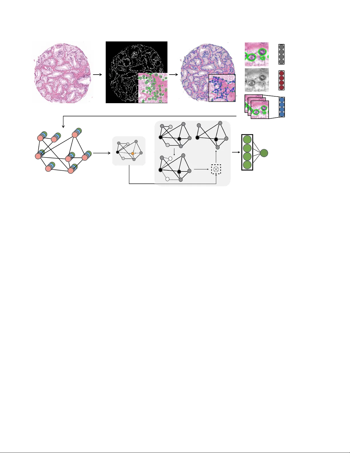
WEAKL Y SUPER VISED PR OST A TE TMA CLASSIFICA TION VIA GRAPH CONV OLUTIONAL NETWORKS Jingwen W ang 1 , Richar d J . Chen 1 , Ming Y . Lu 1 , Alexander Bar as 2 , F aisal Mahmood 1 1 Department of Pathology , Brigham and W omen’ s Hospital, Harv ard Medical School, Boston, MA 2 Department of Pathology , Johns Hopkins School of Medicine, Baltimore, MD jwang111@bwh.harvard.edu faisalmahmood@bwh.harvard.edu ABSTRA CT Histology-based grade classification is clinically important for many cancer types in stratifying patients distinct treatment groups. In prostate cancer , the Gleason score is a grading system used to measure the aggressiv eness of prostate can- cer from the spatial organization of cells and the distribution of glands. Howe ver , the subjective interpretation of Glea- son score often suffers from lar ge interobserver and intraob- server variability . Previous work in deep learning-based ob- jectiv e Gleason grading requires manual pixel-le vel annota- tion. In this work, we propose a weakly-supervised approach for grade classification in tissue micro-arrays (TMA) using graph con volutional networks (GCNs), in which we model the spatial organization of cells as a graph to better capture the proliferation and community structure of tumor cells. As node-lev el features in our graph representation, we learn the morphometry of each cell using a contrastive predictiv e cod- ing (CPC)-based self-supervised approach. W e demonstrate that on a fiv e-fold cross validation our method can achiev e 0 . 9659 ± 0 . 0096 A UC using only TMA-lev el labels. Our method demonstrates a 39.80% improv ement over standard GCNs with texture features and a 29.27% improvement over GCNs with VGG19 features. Our proposed pipeline can be used to objecti vely stratify low and high risk cases, reducing inter- and intra-observer v ariability and pathologist workl oad. Index T erms — Gleason Score Grading, Graph Conv olu- tional Networks, Deep Learning, Histopathology Calassifica- tion, Objectiv e Grading, Patient Stratification 1. INTR ODUCTION The subjecti ve interpretation of histology slides is the standard- of-care for prostate cancer detection and prognostication. The commonly used Gleason score, which informs the aggressive- ness of prostate cancer , is based on the architectural pattern of tumor tissues and the distrib ution of glands. Gleason grade ranges from 1 to 5 to suggest ho w much the prostate tissue looks like healthy tissue (lower score) v ersus abnormal tissue (higher score). If the glands are small, discrete and uniform, the Gleason grade is relativ ely lo wer . On the contrary , if the glands are fused or poorly-formed, the Gleason grade is higher . A primary and a secondary grade which range from 1 to 5 are assigned to prostate tissue and the sum of the two grades determines the final Gleason score. Ho wev er , its man- ual assignment is based on visual, microscopy-based e valu- ation of cellular and morphological patterns, which can be extremely error-prone and time-consuming for pathologists and suf fers from interobserver and intraobserver variability [1]. Deep learning has been widely applied to the detection of malignancies in histology images [2, 3, 4]. Researchers hav e demonstrated that con volutional neural networks (CNNs) can serve as a tool for automated histology image classifi- cation [5, 6, 7], including Gleason score assignment, which alleviates the aforementioned limitations of subjective inter- pretation. Howe ver , CNNs are not sufficiently context-aw are and do not capture the dense spatial relationships between cells that are predictive of cancer grade and proliferation. In addition, CNN-based methods require detailed pixel or patch lev el annotations which are tedious and time consuming to curate [8]. On the contrary , graphs are a reasonable and natural op- tion to model the distribution of the cells in histopathology images. With the cells as nodes and the edges generated by a proper algorithm, graphs can accurately capture the distribu- tion of cells and the spatial relations between the cells. GCN is a deep learning approach for performing feature extrac- tion and classification on graphs[9]. In this paper , we pro- pose a GCN based-approach for automatic patient stratifica- tion trained using TMA-lev el labels and node features learned via a self-supervised technique known as contrastiv e predic- tiv e coding (CPC) [10, 11]. GCNs can learn from the global distribution of cell nuclei, cell morphometry and spatial fea- tures without requiring exhausti ve pix el-lev el annotation. 2. RELA TED WORK Objective Gleason score grading: Previous work on computer-aided Gleason score grading has used machine learning with pixel-le vel annotations. Khurd et al. [12] have dev eloped a texture classification system for automatic and reproducible Gleason grading. They use random forests to cluster extracted filter responses at each pixel into basic tex- ture elements (te xtons) and characterize the te xture in images belonging to a certain tumor grade. del T oro et al. [13] stratify the patients into high-risk and low-risk with the deci- sion boundary of Gleason score 7-8. The y train a CNN that requires pixel-le vel labels on regions of interests (R OI) ex- tracted from WSIs and are able to detect prostatectomy WSIs with highgrade Gleason score. Arvaniti et al. [8] present a deep learning approach for automated Gleason grading of prostate cancer TMAs and are able to assign both the primary score and secondary score to a single pixel in the patients’ TMAs. Ho we ver , all current methods require pixel or patch lev el labels and do not incorporate the spatial organization of cells to fullt capture the archite xture of the tumor micro- en vironment. Classification using GCNs: GCNs proposed by Kipf et al. [9] has been utilized in many classification tasks. Recently , Zhou et al. [14] propose using GCN for colorectal cancer classification, where each node is represented by a nucleus within the original image and cellular interactions are denoted as edges between these nodes according to node similarity . Then they extract spatial features like the centroid coordinates and texture features like angular second moment (ASM) ob- tained from grey le vel co-occurrence matrix (GLCM) [15, 16] for each nodes. GCNs are utilized to classify each image into normal, low-grade and high-grade based on the degree of gland dif ferentiation. Anand et al. [17] also propose to classify cancers using GCNs by modeling a tissue section as a multi-attributed spatial graph of its constituent cells. The y not only extract the spatial and texture features but also use a pre-trained VGG19 model to generate features from a win- dow of size 71 × 71 around the nuclei centroids. Then, a GCN is trained on the breast cancer BA CH dataset [18] to classify patients into cancerous or non-cancerous. Howe ver , these methods rely on gray-scale on ImageNet features and do mot use unsupervised features. 3. METHODS Our idea is inspired by the process through which pathol- ogists examine prostate TMAs and assign Gleason scores. The pathologists inspect the spatial distrib utions of the glands in TMAs. In order to model the distribution of the nuclei, we segment out the nuclei, and then construct the graphs for TMAs with nuclei as the nodes and the potential connection between neighbor nuclei as the edges. With the carefully con- structed cell graphs, we are able to apply GCNs and obtain the stratification results. 3.1. TMA Graph Construction In order to capture the information stored in prostate TMAs, the images first need to be stain-normalized to remo ve the color v ariance. Then, each images is con verted to a cell graph where the nuclei are the nodes and the possible interactions are the edges. W e constructed a graph for each TMA using the following steps: i) segmenting the nuclei, which form the set of nodes. ii) modeling interactions between nuclei using edges. iii) generating features for each node. Nuclei Segmentation: T o detect atypical and packed nuclei and other features that suggest cancerous tissues, precise seg- mentation results are fundamental. Fully con volutional neu- ral networks (FCNN) have been used for nuclei segmenta- tion in the past, which aims to minimize pixel-wise loss [19]. Howe ver , this can sometimes leads to the fusion of nuclei boundaries and these blurry outlines of nuclei can cause fea- ture extraction and graph structure construction to be inaccu- rate. In order detect the nuclei robustly and clearly , we uti- lize conditional GANs (cGANs) [20]. Such methods, which use an proper loss function for semantic segmentation, have been prov ed to a void the aforementioned issues. W e train our model for segmentation on the Multi-Organ Nuclei Segmen- tation dataset [21]. This dataset, which consists of 21,623 nuclei in 30 images, comes from 18 dif ferent hospitals and include di verse nuclear appearances from a v ariety of organs like li ver , prostate, bladder , etc. Nuclei Connection: W e assume that nuclei that are close to each other are more likely to hav e interactions and we intend to capture the architectural structure between neighboring nu- clei. Based on this idea, we adopt the K -nearest neighbors (KNN) algorithm[22], in which each nucleus is connected to its top 5 nearest neighboring nucleus if they are within a cer- tain Euclidean distance (100 pixels in our method). Nuclei Feature Extraction: Based on the nuclei masks ob- tained using a cGAN, we then extract both morphological and texture features for each nucleus, along with features ex- tracted from CPC-based self-supervise learning. • Morphological Features: For morphological features, we compute area, roundness, eccentricity , conv exity , orienta- tion, etc for each of the nucleus. • T exture Featur es: T o analyze the nuclei te xture in the TMAs, we calculate GLCM for each nucleus and then com- pute second order features like dissimilarity , homogeneity , energy and ASM based on the obtained GLCM. • Contrastive Predictive Coding Features: Contrastiv e predictiv e coding is an unsupervised learning approach to extract useful representations from high-dimensional data. By predicting the future in the latent space, CPC [11] is able to learn such representations through autoregressi ve models. W ith a certain data sequence { x t } , a feature net- work g enc first calculates a low-dimensional embedding z t for each observ ation. Then, an auto-regressi ve context net- work g c can accumulate observations prior to t , namely , c t = g c ( { z i } ) , for i ≤ t . CPC utilizes a contrastiv e loss, through which the mutual information shared between the context c t , the present, and future observations z t + k , k > 0 can be maximized. The network aims to correctly distin- guish the positive target z t + k from sampled negati ve can- didates. Predictions for z t + k can be achie ved linearly us- ing weights W k : ˆ z t + k = W k c t . If the probability score for Pros tate TMA Nuclei Segmenta tion TMA Graphs Graph R epresent ation Graph Con volutional Network Fully Connected La yer High-risk or Low-risk T exture fea tures CPC fea tures Morphological fea tures + + Fig. 1 . For cell identification nuclei are segmented in each TMA and a graph is built on the centeroid of each nuclei using the K-nearest neighbours (KNN) algorithm. Morphological, texture and contrastive predictiv e coding (CPC) features are then extracted for each nucleus and GCNs are applied on the graph representation. Finally , a fully connected layer is used at the end for classification. each candidate z i is assigned through a log-bilinear model, the CPC objecti ve is just the standard cross-entropy loss for the positiv e target. When applying CPC to images, small, ov erlapping patches need to be extracted from each image. W e train a CPC encoder on extracted TMA patches of size 256 × 256 and a stride of 128. W e then use the trained model to extract features from a window of size 64 × 64 around the centroid of each detected nucleus. When applying CPC to prostate TMAs at the scale of 256 × 256 patches, we expect that the context (summarized from ro ws of features that are visible to the network) and unknown future observations (ro ws of features hidden from the network) are conditionally dependent on shared high- lev el information specific to the underlying pathology and the tissue site at this resolution. Examples of such high- lev el information might include the morphology and dis- tinct arrangement of dif ferent cell types, the tissue texture and micro-en vironment, etc. By minimizing the CPC ob- jectiv e in the latent space, we implicitly encourage learning of such shared high-le vel abstractions specific to prostate tissue, which one is unlikely to effecti vely capture by us- ing features extracted through naiv e transfer learning from ImageNet. For each nucleus in a prostate TMA, we generate 8 mor- phological features, 4 texture features from GLCMs and 1024 features from CPC. Then, we concatenate them together to form a feature matrix V ∈ R N i × F where N i is the number of nuclei in the graph and F is the number of features (1036 in our method). 3.2. Graph Con volution Networks While CNNs remain a powerful deep learning tool for med- ical image analysis, they can only perform on grid-like Eu- clidean data like 2-dimensional images. Studies hav e been exploring how to generalize con volutional networks onto non- Euclidean domains. Con volution operators have been refined by Kipf et al. [9] to perform on non-grid-like data as graphs like protein structure and nuclei distribution. Through mes- sage passing, each node is able to iteratively accumulate fea- ture vectors from its neighboring nodes and generate a new feature vector at the next hidden layer of the network, thus GCNs can learn to represent for each feature in a node. This process is very similar to feed-forward networks or CNNs. Then, by pooling over all the nodes, we are able to achie ve the presentation for the entire graph. Such graph presentation can then serv e as inputs for tasks as graph-level classification. In our method, we used the GraphSAGE conv olution [23]. The con volution and pooling operations can be defined as fol- lows: a ( k ) v = MAX n ReLU  W · h ( k − 1) u  , ∀ u ∈ N ( v ) o h ( k ) v = W · h h ( k − 1) v , a ( k ) v i At the ( k − 1) th iteration of the neighborhood accumula- T able 1 . A comparativ e analysis of prostate TMA classification using various models and features. Model Accuracy ↑ A UC ↑ GCN + GLCM features 0.6299 ± 0.0391 0.6909 ± 0.0240 GCN + GLCM + T ransfer Learning (ResNet56) 0.6412 ± 0.0181 0.6987 ± 0.0294 GCN + GLCM + T ransfer Learning (VGG19) [17] 0.7194 ± 0.1192 0.7486 ± 0.0377 GCN + GLCM + CPC features (Pr oposed) 0.8995 ± 0.0222 0.9659 ± 0.0096 tion, the feature v ector for node v is denoted by h ( k ) v while the feature vector of node v at the next iteration is represented by a ( k ) v . For the pooling part, we utilize the self-attention graph pooling method [24]. Self-attention can reduce computational complexity and take the topology into account. By perform- ing self-attention graph pooling, our method is able to cal- culate attention scores, focus on the more meaningful node features and aggregate information of nuclei graph topology on different lev els. The attention score Z ∈ R N × 1 for nodes in G can be calculated as follo ws: Z = σ  SA GECon v  X, A + A 2  The node features are represented by X , the adjacency ma- trix is suggested by A , while SA GECon v is the con volution operator from GraphSA GE. 4. EXPERIMENTS AND RESUL TS W e train both the CPC and the GCN on a high-resolution H&E stained image dataset from 5 prostate TMAs, each con- taining 200-300 spots [25, 26]. There are 886 images in total. For each image, there is a pixel-lev el annotation mask sug- gesting the Gleason scores. In order to obtain the TMA-le vel labels, we calculate the primary grade and secondary grade based on the area in the mask and sum up the two grade to- gether as the final Gleason score. For data augmentation, we took 1550 × 1550 crops from the four corners and the center of each image, and computed their corresponding binary la- bels. The crops that do not contain tissue are discarded. W e classify the TMAs with Gleason score higher than (including) 6 as high-risk while TMAs with Gleason score lower than 6 as lo w-risk. Gleason scores of 3 + 3 and 3 + 4 are known to have the most interobserver and intraobserver variability [27] and our proposed method can stratify between the two highly variable scores. W e v alidate our approach on 5 class- balanced splits where each splits contain 3498 crops for train- ing, 388 crops for validation and 432 crops for testing. T able 1. shows a comparative analysis of our proposed method with other methods in a fiv e-fold cross v alidation. For comparison, we trained GCNs with the features gen- erated from GLCMs, ResNet56 and VGG19 in contrast to the features generated from CPC. Results show GCNs with a combination of GLCM and CPC features achiev e state-of- the-art results with an A UC of 0.9659. Fig. 2 . Comparati ve analysis of our approach (GCN with GLCM+CPC features) as compared to other approaches demonstrates that our method achie ves a 39.80% higher A UC ov er GCNs with just GLCM features and a 29.27% improv e- ment over GCNs with VGG19 features. The shade suggests the confidence interval from the 5 random cross v alidation 5. CONCLUSIONS In the paper , we propose an approach for using GCNs as a tool to stratify patients on prostate cancer . Our approach is able to accurately identify high-risk patients using the prostate TMAs with only the image-level labels instead of the pixel- lev el labels. Also, we demonstrate that using CPC features in graph con volution can outperform features generated through simple transfer learning from ImageNet. Our deep learning-based TMA stratification pipeline can be used as an assisti ve tool for pathologists to automatically stratify out high-risk cases before re view . This work has the potential to alleviate the overall pathologist burden, acceler- ate clinical workflo ws and reduce costs. Future work will in- volv e scaling this to a six class classification problem, iden- tifying nodes being activ ated for interpretability and fusing information from patient and familial histories and incorpo- rating multi-omics information for improved diagnostic and prognostic determinations. W e will also explore methods to scale this to whole slide images. 6. REFERENCES [1] Thomas J Fuchs and Joachim M Buhmann, “Computational pathology: Challenges and promises for tissue analysis, ” Com- puterized Medical Imaging and Graphics , v ol. 35, no. 7-8, pp. 515–530, 2011. [2] Geert Litjens, Clara I S ´ anchez, Nadya Timofee va, Meyk e Hermsen, Iris Nagtegaal, Iringo K ovacs, Christina Hulsber gen- V an De Kaa, Peter Bult, Bram V an Ginneken, and Jeroen V an Der Laak, “Deep learning as a tool for increased accuracy and efficienc y of histopathological diagnosis, ” Scientific r eports , vol. 6, pp. 26286, 2016. [3] Rasool Fakoor , Faisal Ladhak, Azade Nazi, and Manfred Hu- ber , “Using deep learning to enhance cancer diagnosis and classification, ” in Pr oceedings of the international conference on machine learning . A CM New Y ork, USA, 2013, vol. 28. [4] Anant Madabhushi and George Lee, “Image analysis and ma- chine learning in digital pathology: Challenges and opportuni- ties, ” 2016. [5] Farzad Ghaznavi, Andre w Ev ans, Anant Madabhushi, and Michael Feldman, “Digital imaging in pathology: whole-slide imaging and beyond, ” Annual Review of P athology: Mecha- nisms of Disease , vol. 8, pp. 331–359, 2013. [6] Y ani v Bar , Idit Diamant, Lior W olf, Siv an Lieberman, Eli K o- nen, and Hayit Greenspan, “Chest pathology detection using deep learning with non-medical training, ” in 2015 IEEE 12th International Symposium on Biomedical Imaging (ISBI) . IEEE, 2015, pp. 294–297. [7] Mehmet G ¨ unhan Ertosun and Daniel L Rubin, “ Automated grading of gliomas using deep learning in digital pathology images: A modular approach with ensemble of con volutional neural networks, ” in AMIA Annual Symposium Pr oceedings . American Medical Informatics Association, 2015, vol. 2015, p. 1899. [8] Eirini Arvaniti, Kim S Fricker , Michael Moret, Niels Rupp, Thomas Hermanns, Christian Fankhauser , Norbert W e y , Peter J W ild, Jan H Rueschoff, and Manfred Claassen, “ Automated gleason grading of prostate cancer tissue microarrays via deep learning, ” Scientific r eports , vol. 8, 2018. [9] Thomas N Kipf and Max W elling, “Semi-supervised classi- fication with graph con volutional networks, ” arXiv pr eprint arXiv:1609.02907 , 2016. [10] A ¨ aron van den Oord, Y azhe Li, and Oriol V inyals, “Represen- tation learning with contrasti ve predicti ve coding, ” CoRR , vol. abs/1807.03748, 2018. [11] Ming Y Lu, Richard J Chen, Jingwen W ang, Debora Dillon, and Faisal Mahmood, “Semi-supervised histology classifica- tion using deep multiple instance learning and contrastive pre- dictiv e coding, ” arXiv pr eprint arXiv:1910.10825 , 2019. [12] Parmeshwar Khurd, Claus Bahlmann, Peter Maday , Ali Ka- men, Summer Gibbs-Strauss, Elizabeth M Geneg a, and John V Frangioni, “Computer-aided gleason grading of prostate can- cer histopathological images using texton forests, ” in 2010 IEEE International Symposium on Biomedical Imaging: F r om Nano to Macr o . IEEE, 2010, pp. 636–639. [13] Oscar Jim ´ enez del T oro, Manfredo Atzori, Sebastian Ot ´ alora, Mats Andersson, Kristian Eur ´ en, Martin Hedlund, Peter R ¨ onnquist, and Henning M ¨ uller , “Con volutional neural net- works for an automatic classification of prostate tissue slides with high-grade gleason score, ” in Medical Imaging 2017: Digital P athology . International Society for Optics and Pho- tonics, 2017, vol. 10140, p. 101400O. [14] Y anning Zhou, Simon Graham, Na vid Alemi K oohbanani, Muhammad Shaban, Pheng-Ann Heng, and Nasir Rajpoot, “Cgc-net: Cell graph conv olutional network for grading of colorectal cancer histology images, ” arXiv preprint arXiv:1909.01068 , 2019. [15] Fritz Albregtsen et al., “Statistical texture measures computed from gray lev el coocurrence matrices, ” Image processing lab- oratory , department of informatics, university of oslo , vol. 5, 2008. [16] P Mohanaiah, P Sathyanarayana, and L GuruKumar , “Image texture feature extraction using glcm approach, ” International journal of scientific and resear ch publications , v ol. 3, no. 5, pp. 1, 2013. [17] Shrey Gadiya, Deepak Anand, and Amit Sethi, “Histographs: Graphs in histopathology , ” arXiv preprint , 2019. [18] Guilherme Aresta, T eresa Ara ´ ujo, Scotty Kwok, Sai Saketh Chennamsetty , Mohammed Safwan, V arghese Alex, Bahram Marami, Marcel Prastawa, Monica Chan, Michael Donovan, et al., “Bach: Grand challenge on breast cancer histology im- ages, ” Medical image analysis , 2019. [19] Peter Naylor , Marick La ´ e, Fabien Reyal, and Thomas W al- ter , “Nuclei segmentation in histopathology images using deep neural networks, ” in 2017 IEEE 14th International Symposium on Biomedical Imaging (ISBI 2017) . IEEE, 2017, pp. 933–936. [20] Faisal Mahmood, Daniel Borders, Richard Chen, Gregory N McKay , K ev an J Salimian, Alexander Baras, and Nicholas J Durr , “Deep adversarial training for multi-organ nuclei seg- mentation in histopathology images, ” IEEE tr ansactions on medical imaging , 2019. [21] Neeraj Kumar , Ruchika V erma, Sanuj Sharma, Surabhi Bhar- gav a, Abhishek V ahadane, and Amit Sethi, “ A dataset and a technique for generalized nuclear segmentation for computa- tional pathology , ” IEEE T ransactions on Medical Imaging , v ol. 36, no. 7, pp. 1550–1560, July 2017. [22] Sahibsingh A Dudani, “The distance-weighted k-nearest- neighbor rule, ” IEEE T ransactions on Systems, Man, and Cy- bernetics , , no. 4, pp. 325–327, 1976. [23] Will Hamilton, Zhitao Y ing, and Jure Leskov ec, “Inductiv e representation learning on lar ge graphs, ” in Advances in Neural Information Pr ocessing Systems , 2017, pp. 1024–1034. [24] Junhyun Lee, Inyeop Lee, and Jaew oo Kang, “Self-attention graph pooling, ” arXiv pr eprint arXiv:1904.08082 , 2019. [25] Qing Zhong, T iannan Guo, Markus Rechsteiner , Jan H R ¨ uschoff, Niels Rupp, Christian Fankhauser , Karim Saba, Ashkan Morteza vi, C ´ edric Poyet, Thomas Hermanns, et al., “ A curated collection of tissue microarray images and clinical outcome data of prostate cancer patients, ” Scientific data , vol. 4, pp. 170014, 2017. [26] Eirini Arv aniti, Kim Fricker , Michael Moret, Niels Rupp, Thomas Hermanns, Christian Fankhauser , Norbert W ey , Peter W ild, Jan Hendrik Rschoff, and Manfred Claassen, “Replica- tion Data for: Automated Gleason grading of prostate cancer tissue microarrays via deep learning., ” 2018. [27] T ayyar A Ozkan, Ahmet T Eruyar, Oguz O Cebeci, Omur Memik, Lev ent Ozcan, and Ibrahim Kusk onmaz, “Interob- server v ariability in gleason histological grading of prostate cancer , ” Scandinavian journal of ur ology , vol. 50, no. 6, pp. 420–424, 2016.