A Machine Learning Nowcasting Method based on Real-time Reanalysis Data

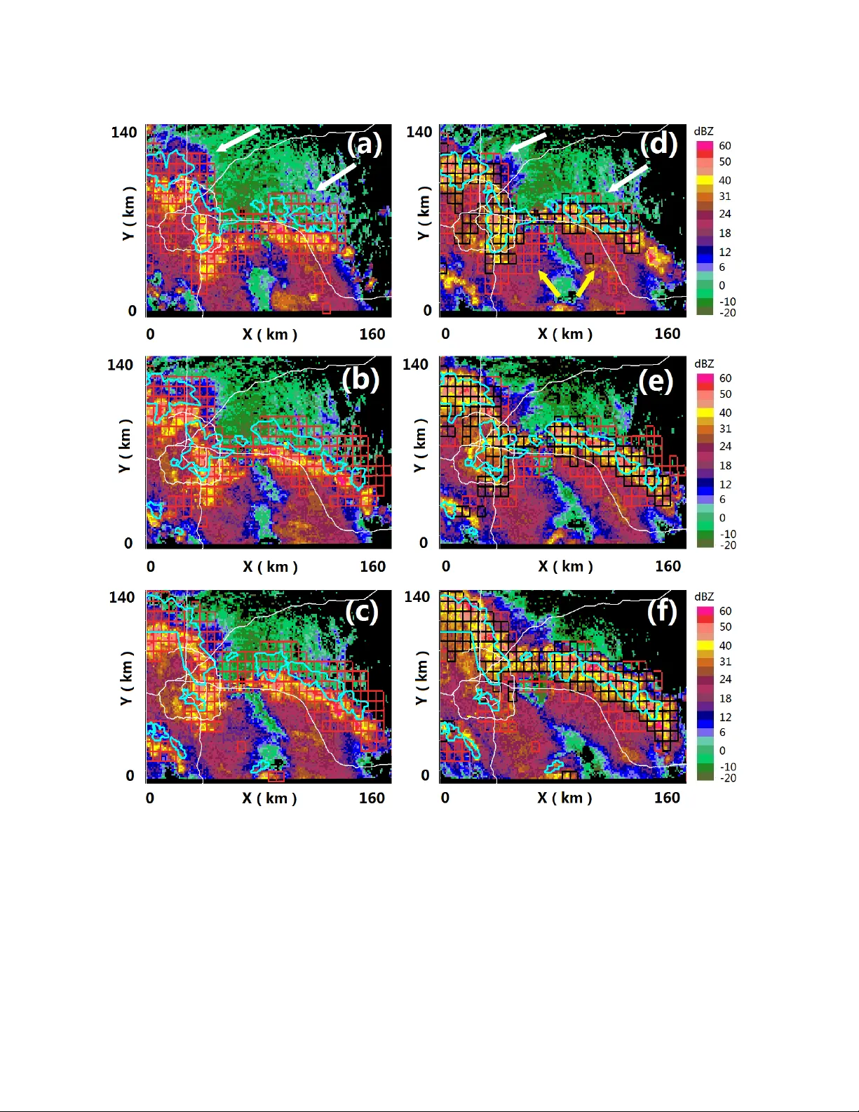
A Machine Lear ning Nowc asting Method bas ed on Real-time Reanalys is Data Lei Han 1,2 , Juanzhen Sun 3 , Wei Zhang 1,2 ,Yuanyuan Xiu 1 , Hailei Fe ng 1 ,and Yinjing Lin 4 1 College of Informatio n Science and Engineering, O cean Universit y of China, Qin gdao, Shandong, China 2 I nstitute of Urban Meteorology, China Meteorological Administration, Beijing, China 3 National Center for Atmospheric Researc h, Boulder, CO 4 National Meteorolog ical Center, China Meteorological Administration, Beijing, China Corresponding author: Juanzhen Sun (sunj@ucar.edu), Wei Zhang (weizhang@ouc.edu.cn) Citation : Han, L., S un, J ., Zhang, W., Xiu, Y., Feng, H., and Lin, Y. (2017), A machine le arning nowcasting method based on realtime reanalysis data, J. Geophy s. Res. Atmos., 122, doi:10.1002/2016JD025783. Abstract Despite marked progress over the past s everal decades, conv ective storm nowcasting remains a challenge because most nowcasting s ystems are based on line ar extrapolation of radar reflectivity without much consideration for other meteorological fields. The variational Doppler radar analysis s ystem (VDRAS) is an advanced convective -scale anal ysis system capable of providing anal ysis of 3 -D wind, temperature, and humidity b y assimilating Doppler radar observations. Although p otentially useful, it is sti ll an open question as to how to use these fields to improve nowcasting . In this study, w e present results from our first attemp t at developing a Support Vector Machine (SVM) B ox-based nOWcasting (SBOW) method under the machine learning framework using VDRAS analysis data. The ke y desig n points of S BOW are as follows: 1) The stud y domain i s divi ded into man y position -fix ed small boxes and the nowcasting problem is transformed into one question, i.e., will a radar e cho > 35 dBZ appear in a box in 30 minutes? 2) Box -based temporal and spatial features, which include time trends and sur rounding environmental information, are constructed; and 3) The box -based constructed features are used to first train the SVM classifier, and then the trained classifier is used to make predictions. Compared with complicated and expensive expert s y stems, the above design of SBOW allows the system to be small, compact, straightforward, and easy to maintain and expand at low cost. The experimental results show that, although no complicated tracking algorithm is used, SBOW can predict the storm movement trend and storm growth with rea sonable skill. 1 Introduction Although the re has been much progress over the past several decades, very short-term           methods can be classified into three categories: extrapolation techniques based on radar data, numerical weather prediction (NWP) models, and knowledge-based ex pert systems that blend NWP and extrapolation techniques [ Wilson et al., 1998, 2010; Sun et al., 2014]. Extrapolation techniques include cross-correlatio n tracking [ Rinehart and Garvey, 1979; Tuttle and Foote , 1990; Li et al., 1995; Lai, 1999] and centroid tracking [ Austin and Bellon, 1982; Rosenfeld, 1987; Handwe rker , 2002; Han et al ., 2009] techniques. Centroid tracking can be used to obtain various properties of a single storm ce ll , such as storm area , volume, top, base, etc. Storm Cell Identification and Tr acking [ SCIT; Johnson et al., 1998] and Thunderstorm Identification, Tracking, and Nowcasting [ TITAN ; Dixon and Wiener, 1993 ] are two well-known centroid-type now casting algorithms. In contrast, the cross- correlation tracking method does not aim at single storm cells, but can provide the mot ion vectors for all radar echoes. Although widely us ed, none of these extrapolation techniques are able to fo recast convective storm initiation, and they have no or only limited ability in forecasting storm growth and decay, thus limiting their nowcasting accuracy [ Dixon and Wiener , 1993; Wilson et al., 2010]. Nowcasting techniques were first developed with radar observations; recently, attemp ts have been mad e to incorporate satellite data using similar techniques as well as passive remote sensing -based techniques, such as inf rared (IR) temperature time-differencing and multispectral IR channel differencing techniques [ Mecikalski and Bedka, 2006; Sieglaff et al., 2011, 2013]. Although there h as been a great deal of progress in the nowcasting application of high - resolution and convection-permitting NWP, it is still far from being adequate for this purpos e [ Weisman et al. , 2008; Sun et al. , 2014]. Man y problems remain to be addre ssed, such as the need for running NWP with model re solutions of less than a few kilom eters, dealing with the spinup problem, rapid model error growth at the convective sca le, etc. The use of expert s ystems that att empt to blend the strengths of extrapolation techniques and NWP , such as Auto -Nowcaster[ ANC; Mueller et al., 2003] , Nowcasting and Initialization of Modelling Using Regional Observation Data S ystem [ NIMROD; Golding, 1998] , and Short- Range Warnin g of Intense Rainstorms in L ocalized Systems [ S WIRL; Y eung et al ., 2009], is becoming incre asingly c ommon [ Wilson et al ., 2010]. However, other than being complicated and requiring input from many data sources as well as lar ge maintenance efforts, these expert systems depend on the f orecast a ccuracy o f NWP models and suffer the same problems as the direct use of NWP for nowcasting. The variational Doppler radar analysis s ystem (VDRAS) is a high-resolution data assimilation s y stem that was designed to retrieve unobserv ed meteorological variables of wind, temperature, and humidity at the convective scale, with frequent updates at int ervals of less than 20 minutes, by assimilating radial ve locity and reflectivit y from single or multiple Dopple r radars [ Sun and Crook , 1997, 2001; Sun et al. , 2010). Because the advanced four -dimensional variational (4DVAR) d ata assimilation technique is used with a cloud -model (which is its constraint over a short assimi lation window), VDRAS is able to p roduce frequently updated analysis in a d ynamically consistent manner. I n addition to radar data, VDRAS can also assimilate data from in-s itu observations, such as radiosondes, profilers, surface networks, VAD analysis, and mesoscale model analysis. Over the past several decades, V DRAS has bee n run in many w eather service offices throughout the world and has prove n to be an effective tool for providing useful real-time information to nowcast convective weather. As VDRAS analysis are highly dependent on high-resolution radar observations, the y have been shown to be quite accurate in convective situations [ Sun et al. 2010]. The retrieved meteorological fields have been used directly b y forecasters, and as input into ex pert systems to nowcas t storm initiation and location [ Mueller et al ., 2003]. In this paper, we describe a new method of using VDRAS analysis for thunderstorm nowcasting. The method employs VDRAS anal y sis data to build a Support vector machine Box - based nowcastin g (SBOW ) algorithm under the machine -learning framework. S BOW constructs box-based temporal an d spatial features, wh ich includes time trends and surrounding environmental information. These box -based co nstructed f eatures are used to train the support vector machin e (SVM) classifier and then the trained classifier is us ed to mak e predictions. Th e concise design of S BOW makes the system small, compact, str aightforward, and eas y to maintain and expand at low cost. Onl y VDRAS and radar data are ne eded. In this study, we used VDRAS analysis of five heavy rainfall/flash flood cases th at occurred in eastern Colorado to train the system; two sim ilar cases w ere then used for the p redictions. The nowcasting skill of SBOW was v erified against radar observations. The experimental results showed that, although we used no complicated trac king algorithm, SBOW could predict storm movement trends and storm growth with reasonable skill. Although in the current stud y SBOW was applied to VDRAS analysis data to sho w its potential, the method can be a pplied to any other meteo rological analysis datasets. This pa per is organized as follows. S ection 2 describes the d ata used in this study . Section 3 introduces the methodology, and Section 4 describes the anal ysis results of case studies. Finally, the conclusions are presented in Section 5. 2 Data The data used in this stud y in cludes reflectivit y data from the KFTG WSR -88D radar located in Denver, USA and VDRAS analysis data. The KFTG reflectivit y data were also used to verify the nowcasting results. For the convenience of data processin g, the radar reflect ivity data were transformed from spherical coordinates into Cartesian coordinates with a horizontal spatial resolution 0.01° × 0.01° (about 1 km × 1 km) and a vertical resolution 1 km. The grid resolution of the VDRAS data used in this study was3 km in the horizontal direction and 300 m in the vertical direction with a grid mesh of 280 × 230 × 20. The interval of two successive VDRAS outputs is 15 minutes. For consistency with the radar data, all VDRAS data were interpolated into the same grid as radar data with a horizontal spatial resolution of 0.01° . The radar and VDRAS data of seven historic heav y rainfall events in the Colorado front range area o f the R ocky Mountains used in thi s study (8  9 Au gust 2008, 28  29 J uly 2010, 9  10 August 2010, 13  14 July 2011, 14  15 July 2011, 6  7 June 2012, and 7  8 July 2012) were collected from a retrospective stud y of hist orical heav y rain/flash flo od cases conducted b y the Short Term Ex plicit Prediction (STEP) Program of NCAR. STEP is a multi -NCAR laboratory activit y aimed to improve the short-term forecasting of high -impact weather, such as severe thunderstorms, winter storms, and hurricanes (http://www.rap.ucar.edu/projects/step/). Figure 1 shows the VD RAS analysis domain and our study domain. The smaller s tud y domain was chosen to elimi nate near-boundary areas and high mo untain regions whe re observations were scarce. The VDRAS analysis data includes basic meteorological fields with three velocit y components: temperature, humidity, and microph ysics, and deri ved fields such as divergence. Figure1. The V DRAS analysis domain and the stud y domain (red r ectangle). The location of the KFTG radar near Denver is shown by the red cross. The green lines indicate the state borders and the white lines are the major highways. 3 Methodology The key design features of the SBOW alg orithm are as follows: 1) the whole method is based on small boxes. The study domain is divided into man y position-fixed small box es, and the nowcasting problem is transformed into one question, i.e., will a radar echo > 35 dBZ appear in a box in 30 minutes? 2) box-based temporal and spatial f eatures, which include time trends and surrounding environmental information, are constructed and 3)a machine l earning framework is applied to perform the n owcasting task, i.e., the box -based constructed features are used to train the SVM classifier first, and the tr ained classifier is then used to make p redictions. It should be noted that in this stud y we divide all the data in to three independent sub sets for training, cross validation, and testing, respectively. Figure 2 presents an overview of the flow o f the algorithm. Th e overall method consists of three main components: 1) box -based temporal feature construction; 2) box -based spatial feature construction; and 3) application of SVM, a powerful machine lea rning m ethod, to train the classifier and make 30-min forecasts. These components are de scribed below. Figure2. Flowchart of the SBOW algorithm. 3.1 Box-based temporal feature construction The first step in developing the SBOW algorithm was to select candidate features or predictors that could be used for training. Among the anal ysis variables of VDRAS, we first chose vertical wind (w) and the perturbation temperature ( pt , subtracted from the horiz ontal mean), which is proport ional to the buoyancy. W e then constructed the temporal features of their time trends, i.e., dw and dpt , respectively. The four variables we re used in the SBOW algorithm as the candidate predictors. Vertical velocit y is closel y related to the low -level convergence and plays an important role in storm initiation and development [ Wilson and Mueller , 1993]. A large value of w indicates strong lifting, which is one of the n ecessary ingredients to achieve deep convection [ Doswell , 1992]. Buoyancy represents the vertical acceleration of an air parcel resultin g from an unstable atmosphere. It is the driving force and pl ays a ke y role in deep convection [ Wallace and Hobbs 1977]. The temporal trend contains information about storm growth/deca y and thus can also pla y an important role in convective no wcasting. [ Roberts and Rutledge , 2003; Mecikalski and Bedka , 2006; Sieglaff et al., 2011] have shown that satellite infrared ( IR) cloud-top temperature trend information is very useful in forecasting convective initiation. Instead of computing w, pt, dw , and dpt at each p ixel, these feature s were computed in a 3D box (0.06° × 0.06° , 20 levels). The values of w and pt are calculated first. Particularly, w is                     pt is the maximum value above 4 km in the 3D bo x. The choice of the vertical la yers for w an d pt , although being somewhat arbitra ry, is based on the consideration that the lower level vertical velocity and hi gher-level latent hea ting could play greater roles in convective initiation. After obtaining w and pt in each box at each ti me step, dw and dpt can be determined by computing their respective differences between current and previous time steps. Therefore for each box at a time step, we can obtain four features: w, pt, dw, and dpt. (a ) Trai ni n g ra dar d ata as the labe l VDR AS Data Tempo ral & Spatial Fea ture cons truct ion SVM Traini ng f eature s (b) Pred i c tion Traine d Clas sif i er Forecas t Result New V DRA S D a ta Tempo ral & Spatial Fea ture cons truct ion f eature s 3.2 Box-based spatial feature construction Weather phenomena are not only continuous in time but also in space, i.e., each box is impacted by it s neighboring boxes, so it is necessary to construct spatial features to take these impacts into account. As shown in Figure 3, e ach box has four features ( w, pt, dw, dpt ). However, instead of only assigning its own four features to the box located at ( i, j ), we also assigned the same features of its neighboring eight box es. Thus, ther e ar e 4 × 9 = 36 features for the box located at ( i, j ), and the same is true for all other boxes. Th is allows the SBOW algorithm to consider the surrounding information around the center box, which can be importa nt for a successful nowcast. Although we believe th at our choice of the four c andidate predictors has a good ph ysical basis, there could be other predictors that would be useful to help improve the nowcast, for example, moi sture, verti cal wind shea r, et c. But it is well known that, in most instances, SVM classifiers are more accurate with some feature reduction. More features do no t mean better classification performan ce. We performed a greedy feature selection, i.e. the feature set was initialized from empty s et first, and then we iteratively added one feature that maximized the classification performance among the rest features. { w, pt, dw , dpt } was finally selected. Figure3. Illustration of box-based spatial feature construction. The surrounding box es used for additional spatial features are indicated by the blue color. 3.3 Application of SVM SVM is a supervised learning method. Through learning from a labeled tr aining dataset, it c onstructs an optimal hyperplane in a high-dimensional spac e for classification [ Boser et al . 1992; Cortes and Vapnik , 1995; Vapnik, 1998]. SVM has become a mature, powerful tool and been used in atmospheri c research [ Lee et al., 2004; Mercer et al. , 2008 ; Felker et al. , 2011; Zhuo et al. 2014]. 3.3.1 Description of SVM ( i , j+ 1 ) ( i-1 , j+ 1 ) ( i-1 , j - 1 ) ( i-1 , j ) ( i , j ) ( i , j- 1 ) ( i+1 , j- 1 ) ( i+1 , j ) ( i+1 , j+ 1 ) The basic SVM is a two-class classifier. Given a training set with n dim ensional feature vectors      and its corresponding label    󰇝󰇞 , SVM solves the following optimization problem [ Chang and Lin , 2011 ]: 󰇛                󰇜 (1) subject to   󰇛    󰇛   󰇜   󰇜                 where  󰇛   󰇜 maps   into a higher dimensional space and  is the penalt y p arameter of the error term.          󰇛   󰇜     is defined as the kernel function. W e use the radial basis function (RBF) kernel:          󰇛        󰇜    (2) where  is kerne l par ameter. The pair of penalt y and kernel parameter, (   󰇜  󰇛   󰇜 , is chosen b y a grid search on the 5-fold cross validation (5-CV) of the traini ng s et [ Chang and Lin , 2011 ]. This grid search iterativel y test classification performance on 5 -CV for values of C (2 -5 , 2 - 4 , 2 -3 ,..., 2 15 ) and RBF kernel parameter γ (2 - 15 , 2 - 14 , 2 - 13 ,..., 2 3 ). Among commonl y used kernels, besides RBF, the polynomial kernel is also an option. But for our stud y, the RBF kernel performs better. It should be noted that VDRAS, being a 4DVAR method, also suffers from NW P model errors, and thes e errors will therefore de grade the nowcasting algorithm performance. However, a major strength of machine learning methods is that the y could potentia lly mitigate the effects of sy stemic NWP model errors or observation errors. This strength sources from the generalization abilit y of machine learning [ Bishop 2006; Mohri et al . 2012] . A core objective of a classifier is to generalize from its e xperience. Generalization in this context is the ability of a classifier to perform accuratel y on new, unsee n data after constructing a model on training set whilst preventing the model from overfitting to the training set. In the v iew of the structural risk minimization principle of SVM, the generalization is fulfilled b y the regularization term        of the optimization function: 󰇛                󰇜 [ Vapnik a nd Chervonenkis , 1971; Vapnik, 2000 ]. Use of SVM consists of two steps: training a nd prediction. The y are described below. 3.3.2 Training The stud y domain was d ivided int o 1,209 boxes. If there are 10 time lev els of VDRAS dataset for one convective weather event, the total number of box es will be 12,090. At each time level, each box has 36 features, including four features from the box itself, and another 32 features from its neighboring eight boxes. For training purposes, it is n ecessary to label each box. For a box at time t, if there is a radar echo > 35 dBZ at time t + 30 mi nutes, this box is labeled                    We used five historic h eavy rainfall/flash flood events ov er the Front Range area for training (8  9 August 2008, 28  29 July 2010, 9  10 August 2010, 13  14 July 2011, 14  15 Jul y 2011), and obtained 195,858 labeled boxes as the tr aining and validation datas et. Each labeled box has 36 features. Each feature is scaled to [-1,1] by the min-max normalization.                question: given the 36 feature s of a box , will a radar ec ho > 35 d BZ ap pear in this box in 30 minutes? 3.3.3 Prediction With the trained SVM classifier, when given new VDRAS data, we could use this classifier to make predictions. For example, at time t, when new VDRAS data arrive, it is divided into 1,209 boxes and the 36 feature s are calculat ed for each box . These 36 feature s are used as inputs into the trained SVM classifier. If the output of SVM is 1, we would predict that there will be a convective storm in this box in 30 minutes; this box will be marked as a red rectan gle (examples will be given in the next section). Given the RBF kernel and the size of feature set, the computational cost of applying the trained SVM model mainly depends on the numbe r of support vectors. In o ur case, there are only 18709~19026 support vectors in 5-CV. Typically, it costs onl y ~0.005 seconds to make a prediction for one sample. 4 Experiments and Analysis 4.1 Comparison results of five machine learning methods The contingenc y t able approach ( Donaldson et al. 1975) was used in this study to evaluate the nowcast results. The proba bility of detection (POD), false alarm ratio (FAR) and critical success index (CSI) are calculated. At each box , a success (S) oc curs when this box is classified as 1 (active) and there is a radar echo greater tha n 35 dBZ in the forecast time in th e same box (active), a failure (F) occurs wh en the truth box is active while the forecast box inactive, and a false alarm (A) occurs when the truth box is inactive while the forecast box active. Thus, POD = S/(S + F), FAR = A/(S + A), and CSI = S/(S + F + A) [ Dixon and Wiener 1993]. First, we compare SBOW performance with four other machine learning methods using 5-fold cross validation (5-CV). The other four met hods are: logistic r egression [ Cox, 1958] , J48 , Adaboost and Maxent. Although the last thre e methods are less used by atmospheric scientists , they are well known in machine learning communit y. J 48 is an open source implementation of the C4.5 decision tree al gorithm [ Quinlan , 2014; Frank et al ., 2016]. M axent is a ma ximum entropy modeling method aiming to find the best model   with maximum entropy:       󰇛󰇜 (3) where  󰇛  󰇜 is the conditional entropy of the posterior probability of the data, C is the set of all possible models which satisf y specific feature statist ics [ Jaynes , 1957 ; Phillips et al ., 2004] . Adaboost is an ensemble method that combines a group of weak classifiers to construct a stron g classifier [ Freund and Schapire , 1995 ; Viola and Jones , 2004]. At each iteration t , a weak classifier is s elected and assigned a coefficient   such that the following su m training error   is minimized:      󰇟  󰇛  󰇜        󰇜󰇠 (4) wh ere    󰇛  󰇜 is the classifier th at has been built up to th e previous sta ge o f training,     󰇜 is the weak classifier that is being considered for addition to the final classifier. All methods used the same training data. Each training sample has 36 features. We randomized the sample set by shuffling all sa mples for cross -validation. All instance s were subjected to 5-                  FAR are shown in Table 1. SVM had the hi ghest CS I and POD value and the lowest FAR among all the methods. Table 1 : Comparison of five machine lear ning methods o n 5- CV Approach POD(±  ) FAR(±  ) CSI(±  ) SBOW (SVM) 0.6050± 0.0 0 58 0.5243± 0.0 0 82 0.3631± 0.0064 Logistic Regression 0.5111± 0.0361 0.5799± 0.0360 0.2980± 0.0086 J48 0.5100± 0.0154 0.5336± 0.0177 0.3066± 0.0296 Adaboost 0.5740± 0.0205 0.5892± 0.0062 0.3146± 0.0044 Maxent* 0.5033± 0.0232 0.5880± 0.0253 0.2922± 0.0090 * Maxent is from http://ho mepages.inf.ed.ac.uk/lzha ng10/maxent.ht ml 4.2 Comparison results of SBOW with TITAN 4.2.1 Qualitative Analysis Two heav y rainfall events (6 J une 2012 and 7 J uly 2012) were used to compare the performances of S BOW and T ITAN. For each of the two cases, the SBOW was run for the period between 21UTC t o 00UTC, producing 12 30 -min nowcasts at VDRAS analysis times that were available ever y 15 minutes. The radar composite reflectivity images of these two cases are shown in Figures 4 and 5, respectively , with a 30 -min interval to show the evolution of the systems. I n the following section, a qualitative ana l y sis will be presented, followed by a quantitative analysis, which will together examine the performance of S BOW as compared with TITAN. Figure 4. The KFTG radar composite reflectivity images at (a) 2130, (b) 2200, (c) 2230, (d) 2300, (e) 2330UTC on 6 June, and (f) 0000 UTC on 7 June 2012. Figure 5. Th e KFTG radar composite reflectivit y images at (a) 2130, (b) 2200, (c) 2230, (d) 2300, (e) 2330UTC on 7 July, and (f) 0000 UTC on 8 July 2012. We first present the 30- min forecast results fo r a storm growth case of 7 Jul y 2012 ove r the southeast Denver area. Figure 6 shows the observed radar reflectivity overlaid with SBOW 30- min nowcasts (red box es) and the corresponding verifications (those correctly predicted boxes are marked a s blac k boxes). Cyan pol ygons represent TITAN 30-min nowc asts. The verification shown b y the black boxes in Figure 6(b) confirms that the 30 - min SBOW nowcast agrees well with the radar 35 +dBZ echoes. In comparison, TITAN can only extrapolate th e existing storm (the bottom-left storm in Fig ure 6(a)), and is not able to forecast this dra matic storm growth well. This is typical shortcoming of all extrapolation methods. Figure 6. Radar composite reflectivit y from KFTG; the red boxes represent the 30 -min SBOW nowcasts. Cyan pol ygons represent TITAN 30-min nowcasts. The boxes in the right column are marked in black to repr esent those bein g correctl y predicted b y SBOW . (a). The SBOW and TITAN 30-min nowcasts at issue time, 2 055 UTC 7 J uly 2012. ( b). The same nowcasts superpositioned over reflectivity at verifica tion time 2 125 UTC. The next two figure s ( Figures 7 and 8) show examples of convective initiation. Here w e                   er than 35 dBZ echoes) rather than from an existing storm nearb y with greater than 35 dBZ echoes. The verification on the right panels in both figures shows good agreement between the S BOW nowcast and the observed reflectivit y. Meanwhile, TITAN just extra polates existing storms and misses the newly born storms in front of the old storms. Figure 7. Same as Figure 6 but over a different sub-domain at the 30-min nowcast issue time, 2310 UTC 7 J uly 2012 (a) a nd at verification time, 2340 UTC (b) to show an example of C I nowcast. Figure 8. Same as Figure 6 but over a different sub-domain at the 30-min nowcast issue time, 2210 UTC 6 June 2012 (a) and at verification time, 2240 UTC (b) to sh ow an example of CI nowcast. SBOW is not only able to nowcast the storm growth and the convective initi ation but also the storm propagation. Now we present the 30-minute forecast results for the propa gation of the squall line case of 7 J uly 2012. Figure 9 show s the observed reflectivity of the squ all line overlaid with S BOW and TITAN 30- min nowcasts. Comparing Figures 9 (a) and (d) at 22:55 UTC, we can see that t he SBOW nowcasts can capture the squall lin e advection ver y well (indicated b y the white arrows). This is encouraging be cause the SBOW predicts the squall line movement without the need to calculate the co mputationally expensive motion vectors of the radar echoes as in the extrapolation techniques. The results at 23:10 and 23:25 UTC show that the SBOW nowcasts continue to capture the squall line movement quite well. As a comparison, TITAN also gives a good forecast for thi s case c haracterized mainl y b y linear p ropagation, but its forecast area is much smaller. As will be sho wn in next section, this will lead to a lower POD value. From Figure 9, we can also identify several fa lse alarms in the SBOW nowcast that occurred mainly behind the squall line, as indi cated by the y ellow arrows , althou gh the y decreased with time. These false alarms could be the result of the inadequacy of S BO W in predicting storm deca y due to the limited number of pre dictors used in the cur rent algorithm , which suggests that future improvement of SBOW should include the pr edictors representing storm decay. Opposit e to SBOW, TITAN tends to under-predict the storm areas, resulting in fewer false alarms. Figure 10 shows similar results for the ca se of 6 J une 2012. Figure 9. Same as Figure 6 but over a la rge ar ea to show an example of storm propagation nowcast on 7 July 2012. (a ), (b) and (c) are the SBOW and TITAN 30 -min nowca sts at issue time, 2255, 2310 and 2325 UTC respectively. ( d), (e) and (f) are these same nowcasts superpositioned over reflectivity at verifica tion time 2325, 2340 and 2355 UTC respectivel y. Figure 10. Same as Fi gure 6 but over a large area to show an example of storm propag ation nowcast on 6 June 2012. (a), (b) and (c ) are the SBOW and T ITAN 30-min nowcasts at issue time, 2125, 2210 and 2240 UTC respectively. (d), (e) and (f) are these same nowcasts superpositioned over reflectivity at verification time 2155, 2240 and 2310 UTC respectively. 4.2.2 Quantitative Analysis The overall P OD, FAR, CS I and Heidke S kill Score ( HSS; see Wilks 2011) values for th e 30- min SBOW and T ITAN nowcasts are given in Table 2 for the two s tudied cases. As the 7 Jul y 2012 case is a squall line of linearly propagation, larger convective system, it is not surprising that it achieved higher CS I and HSS scores than that of the 6 J une 2012 case. Table 2 shows that SBOW has s ubstantial higher POD values than T ITAN, but it also has hi gher FAR values, which leads to that both methods h ave very similar CSI values. The performance diagram (Fig. 11) shows more details of this. We can see that TITAN tends to have an underforecasting bias and S BOW tends to have a slight overforecasting bias, which means TI TAN has more misses and SBOW has more false alarms. With regard to HSS, TITAN has hi gher value than S BOW. Although T ITAN only extrapolates existing storms, its foreca st is still reasonable for l arge and stable s yste ms. In this initial study, SBOW sho ws encouraging potential to nowcast CI or storm growth. But usuall y, the verification area of C I or storm growth is ver y small, which means these improvements do not impact the verification values significantly . Table 2. Verification statistics for the SBOW and T ITAN nowcast for the ca se 6 June and 7 July 2012. Note that the verification o f TITAN no wcasts is also performed on the 0.06 ° × 0.06° box. Date POD FAR CSI HSS SBOW TITAN SBOW TITAN SBOW TITAN SBOW TITAN 20120606 0.62 0.52 0.51 0.46 0.37 0.36 0.51 0.53 20120707 0.61 0.54 0.41 0.37 0.43 0.41 0.54 0.58 Figure 11. The performance diagram of SBOW and TITAN. Dashed lines represent bias scores with labels on the outward extension of the line, while labeled solid contours are CS I. Four results are shown: SBOW forecasts (bold red circle, 20120606; bold red triangle, 20120707) and TITAN forecasts (open red circle, 20120606; open red triangle, 20120707) Our qualitative and quantitative evaluations showe d encouraging results in terms of nowcasting convective initiation, growth, and p ropagation. Nevertheless, the results also suggest that problems ex ist, especiall y the problem of f alse alarms behind or at the location of old storms. Further development efforts are required to improve the performance of the S BOW method by choosing features that can predict storm decay. This will be the focus of one of our future research efforts 5 Summary and discussions This study proposed a nowcasting method called S BOW under the machine learnin g framework using real-time VDRAS reanalysis data. SBOW divided the s tudy domain into man y position-fixed small bo xes and attempted to answer the followin g now casting question: will a Pe r for ma n c e Diag r a m Su ccess R at io Probab i l i ty of Detect ion 0. 1 0. 2 0. 3 0. 4 0. 5 0. 6 0. 7 0. 8 0. 9 0. 0 0. 2 0. 4 0. 6 0. 8 1. 0 0. 0 0. 2 0. 4 0. 6 0. 8 1. 0 0.3 0.5 0.8 1 1.3 1.5 2 3 5 10 radar echo > 35 d BZ appear in a box in 30 minutes ? Box -based temporal and spatial features, which include time trends and surrounding environmental information, are constructed. The machine learnin g framework is employed to perform the nowcasting task, i.e., use the box -based constructed features to train a SVM classifier, and then use the trained classifier to make predictions. The above designs of SBOW make the s ystem small, compact, straightforward, and easy to maintain and expand at low cost. Th e only input data for S BOW are radar reflectivity and VDRAS analysis data. T he experimental results showed that, although no complicated tracking algorithm was used, SBOW could predict storm movement and storm growth wi th reasonable skill. The strength of SBOW in comparison with the traditional extrapolation-based nowcast system TITAN is its abilit y in nowcasting the convective initiation and growth as demonstrated both in the qualitative verification and the statistical ly higher POD. SBOW can be expanded to use other model analysis data sources. Although SBOW showed potential in predicting convective initiation and growth, its success is still limited. One reason for this is that the trainin g data for CI cases are still insufficient, which means that the machine learning method cannot acquire enough knowledge to make correct decisions. As the duration of CI constitutes onl y a small proportion of the whole lifetime of a storm, and t he storm area of CI is often very small, it is difficult to collect enough training d ata for CI cases. Another r eason is that numerical models, such as VDRAS, still need improvement to obtain finer retrieval information. For cases of v ery sma ll, isolated storm cells for which SBOW did not perform well, it is likely that resolutions higher than the current 3-km resolution VDRAS analysis will help. False alarms often occur behind or at the location of old storms, e.g., in areas oc cupied by old storms that appear at forecast issue time but disappear at verification time. This is a difficult situation for SBOW in the current design due to the choice of p redictors. Although the use o f temporal trends ( dw and dpt ) could have pla yed a role in predicting storm decay, this is not an adequate explanation. In future studies, we will test other predictors that may be linked to predicting storm deca y. The possible candid ates are downdraft, relative humidit y , and maximum cooling. Adding some other featu res to SBOW, such as humi dity, Convective Available Poten tial Energy (CAPE), and Convective Inhibition (C IN) from VDRAS may also improve nowcast              quantities are multi-scale in nature, it is not as straightforward to define as it was for the exact               to identif y more relevant features that will lead to the improvement of the nowcasting scheme. However, if done incorrectly, adding more features could degrade the re sults [ Lee et al. , 2004]. To improve SBOW, it is important to obtain more VDRAS data, from w hich S VM can acquire more knowledge to enable b etter decisions. This requires running VDRAS operationally on a fixed domain with fixed resolution and configurations. The Beijing Meteorological Bureau (BMB) has been running V DRAS over the last few years operationally, and our plan is to collaborate with BMB to train SBOW with more data. Our ultimate goal is to test our method operationally. Acknowledgments This work was supporte d jointl y b y China Speci al Fund for M eteorological Research in the Public I nterest (grant GYHY201506004), the National Natural Science Foundation of C hina (grant 41405110) and Natural Science Foundation of Shandong Province (grant ZR2016DM05) . All data from this study can be requested from the authors directly. References Austin, G. L., and A. Bellon, 1982: Very-short-range forecasting of precipitation by objective extrapolation of radar an d satellite data. Now casting, K. Browning, Ed., Academic Pr ess, 177-190. Bishop, C. M. 2006: Pattern Recognition and Machine Learning , Springer Boser, B. E., I. Guy on, and V. N. Vapnik, 19 92: A training algorithm for opti mal mar gin classifiers. In Proceedings of the Fifth Annual Workshop on Computational L earning Theory, pages 144-152. ACM Press. Chang, C. C., L in, C. J. 2011. LI BSVM: a library for support ve ctor machines. ACM Transactions on Intelligent Sy stems and Technology (TIST),2(3), 27. Cortes, C., and V. N. Vapnik, 1995: Support-vector networks. Machine learning, 20(3), 273-297. Cox, D. R. 1958: The regre ssion anal ysis of binary s equences. J ournal of the Ro yal Statistical Society. Series B (Methodologica l), 215-242. Dixon, M. and G. W iener, 1993: TITAN: Thunderstorm identification, tracking, analysis and nowcasting  A radar based methodology. J. Atmos. Oceanic Technol., 10 (6): 785-797. Donaldson, R. J., R. M. D yer, and M. J. Kraus, 1 975: An objective evaluation of techniques for predicting sev ere weather events. Preprints, Ninth Conf. on Severe Local Storms, Norman, OK, Amer. Meteor. Soc., 321  326. Felker, S. R ., B. LaCasse, J. S. Ty o, and E. A. Ritchie, 2011: Forecasting Post -Extratropical Transition Outcomes for Tropical C yclones Using Support Vector Machine Classifiers. J. Atmos. Oceanic Technol., 28, 709  719. Frank, E., Mark A. Hall, and Ian H. Witten 2016: The WEKA Workbenc h. Online Appendix for "Data Mining: Practical Machine Learning Tools and Techniques", Morgan Kaufmann, Fourth Edition, 2016. Freund, Y., and Schapire, R. E. 1995: A desicion-theoretic generalization of on-line learning and an application to boosting. In European conference on computational learning theory (pp. 23-37). Springer Berlin Heidelberg. Golding B. W. Nimrod: A s ystem for generating automated ver y short range forecasts . Meteorol. Appl. 1998, 5: 1- 16. Han, L ., S. X. Fu, L . F. Z hao, Y. G. Zheng, H. Q. Wang and Y. J . Lin, 2009: 3D convective storm identification, tracking, and forecasting-A n enhanced T ITAN algorithm. J. Atmos. Oceanic Technol., 26 (4): 719-732. Handwerker, J., 2002: Cell tracking with TRACE3D  a new algorithm. Atmos. Res., 61, 15-34. Jaynes, E. T. 1957: Information theory and statistical mechanics. Phy sical review, 106(4), 620. John R . Walker, Wayne M. MacKenzie J r., J ohn R. Mecikalski, and Christopher P. J e wett, 2012: An Enhanced Geostationary Satellite  Based Convective Initiation Algorithm for 0  2- h Nowcasting with Object Tracking. J. Appl. Meteor. Climatol., 51, 1931  1949. Johns, R. H., and C. A. Doswell III ,1992: Sever e local storms forecasting, Weather Forecast., 7, 588-612. Johnson, J.T., P.L . Mackeen, A. W itt, E.D. Mitch ell, G. Stumpf, M.D. Eilts, and K.W. Thomas, 1998: The Storm cell identification and tr acking algorithm: an enhanced WSR -88D algorithm. Wea. Forecasting, 13, 263-276. Lai, E.S.T., 1999: TREC application in tropical cyclone observation.Proceedings, ESC AP/WMO Typhoon Committee Annual Review, Seoul, The Typhoon Committee, 135  139. Lee, Y., G.Wahba, and S. A. Ackerman, 2004: Cloud Classification of S atellite Radiance Data by Multicategory Support Vector Machines. J. Atmos. Ocea nic Technol., 21, 159  169. Li, L., W. Schmid, and J. Joss, 1995: Nowcasting o f mot ion and growth of precipitation with radar over a complex orography. J. Appl. Meteorol., 34, 1286-1300. Mecikalski, J. R., and K. M. Bedka, 2006: Forecasting convective initiation by monitorin g the evolution of moving cumulus in daytime GOES imagery. Mon. Wea. Rev., 134, 49  78. Mercer, A. E., H. B. Bluestein, and J . M. Brown, 2008: Statistical model ing o f downslop e windstorms in Boulder, Colorado.Wea. Forecasting, 23, 1176  1194. Mohri, M., Rostamizadeh, A., & Talwalkar, A. 2012: Foundations of machine learning. M IT press. Mueller, C., T. S axen,R.Roberts, J .Wilson, T. Betancourt, S.Dettling, N. Oien, and J . Yee, 2003: NCAR Auto-Nowcast system.Wea. Forecasting, 18, 545  561. Quinlan, J. R. 2014: C4. 5: programs for machine learning. Elsevier. Rinehart, R. E., and E. T. Garvey, 1978: Three-dimensional storm motion detection b y conventional weather radar, Nature, 273,287  289. Roberts, R. D., and S. Rutl edge, 2003: Nowcasting storm initiation and growth using G OES -8 and WSR-88D data, Wea. Forecasting, 18, 562  584. Rosenfeld, D., 1987: Objective method for analysis and tracking of convective cells as seen b y radar. J. Atmos. Oceanic Technol., 4, 422-434. Sieglaff, J. M., D. C. Hartung, W. F. F eltz, L . M. Cronce , V. La kshmanan, 2013: A Sat ellite- Based Convective Cloud Object Tracking and Multipurpose Data Fusion Tool with Application to Developing Convection. J. Atmos. Oceanic Technol. 30, 510-525 Sieglaff, J. M., L. M. Cronce, W . F. Feltz, K. M. Bedka, M. J. Pavolonis, and A. K. Heidinger, 2011: Nowcasting convectivestorm ini tiation using satellite-based box-averaged cloud- top cooling and cloud-type trends. J. Appl. Meteor. Climatol., 50,110  126. Sun, J . and N. A. Crook, 1997: D yna mical and mi crophysical retrieva l from Doppler ra dar observations using a cloud model and its adjoint. Part I: Model de velopment and simulated data experiments. J. Atmos. Sci., 54, 1642-1661. Sun, J . and N. A. Crook, 2001: Real-Time L ow-Level W ind and Temperature Anal ysis Using Single WSR-88D Data. Wea. Forecasting, 16, 117  132. Sun, J ., M. Chen, and Y. W ang, 2010: A frequent -updating analysis system based on radar, surface, and mesoscale model data for the Beijing 2008 forecast demonstration project. Wea. Forecasting., 25, 1715-1735. Sun, J., M.Xue, J. W. Wilson, etc., 2014: Use o f NWP for Nowcasting Convective Precipitation: Recent Progress and Challenges. Bull. Amer. Meteor. Soc., 95, 409  426. Tuttle, J. D., and G. B. Foote, 1990: Determination of the boundar y la yer airflow from a single Doppler radar. J. Atmos. Oceanic Technol., 7, 218  232. Vapnik, V. N. 2000: The nature of statistical learning theory. Springer. Vapnik, V. N. and Chervonenkis, A. 1971: On t he uniform convergence of relative frequencies of events to their probabilities". Theory of Probability and its Applications. 16 (2): 264  280. Vapnik, V. N., 1998 : Statistical learning theory . New York: Wiley. Weisman, M. L., C. Davis, W. Wang, K. W. Manning, and J . B. Klemp, 2008:Experiences with 0  36-h Ex plicit Convective Forecasts with the W RF-ARW Model. W ea. Forecasting, 23, 407-437. Wilks, D. S. , 2011: Statistical Methods in the At mospheric Sciences. Third Edition. Academic press. Wilson, J . W . and C. K. Mueller, 1993: Nowcasts of thunderstorm initiation and evolution. Wea. Forecasting, 8, 113  131 Wilson, J .W., N. A. Crook, C. K. Mueller, J . S un and M. Dixon, 1998: Nowcasting Thunderstorms: A Status Report. Bull. Amer. Meteor. Soc., 79, 2079-2099. Wilson, J. W., Y. Feng, and M. Chen, 2010: Nowcasting challenges during the Beijing Ol ympics: Successes, failures, and i mplications for future no wcasting systems. Wea. Forecasting, 25, 1691-1714. Yeung, L. H. Y., W. K. Wong, P. K. Y. Chan , and E. S. T. Lai, 2009: Appli cations of the Hong Kong Observator y Nowcasting S ystem SW IRLS-2 in support of the 2008 Beijing Olympic Games. Proc. Symp. on Nowcasting and Ver y Sho rt Range Forecasting, Whistler, BC, Canada, WMO, 1.5. Zhuo, W ., Z. Cao, and Y. Xiao, 2014: Cloud Classification of Ground-Based Images Using Texture  Structure Features. J. Atmos. Oceanic Technol., 31, 79  92.