Emergent properties of the local geometry of neural loss landscapes

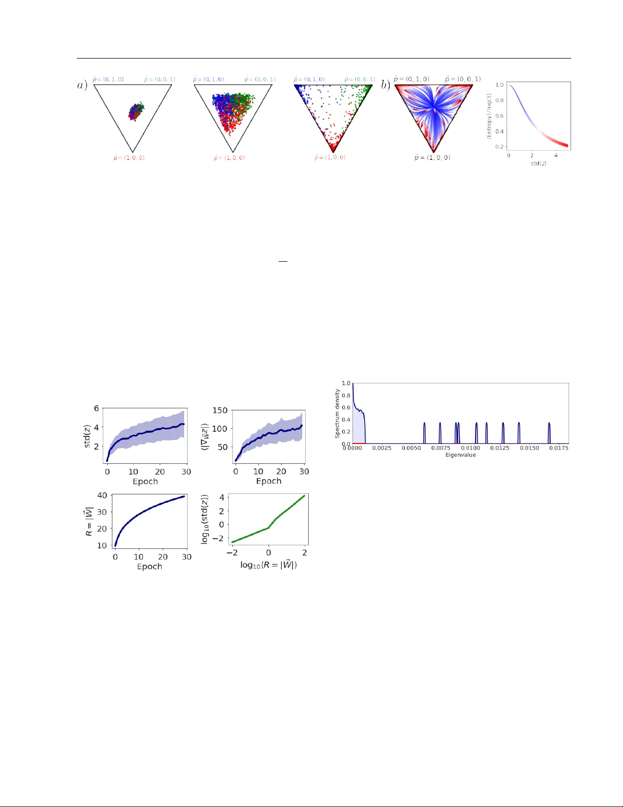
Emergen t prop erties of the lo cal geometry of neural loss landscap es Stanisla v F ort Sury a Ganguli Stanford Univ ersity Stanford, CA, USA Stanford Univ ersity Stanford, CA, USA Abstract The local geometry of high dimensional neu- ral net work loss landscapes can b oth c hal- lenge our c herished theoretical intuitions as w ell as dramatically impact the practical suc- cess of neural netw ork training. Indeed recent w orks hav e observed 4 striking lo cal prop- erties of neural loss landscap es on classifi- cation tasks: (1) the landscap e exhibits ex- actly C directions of high p ositiv e curv ature, where C is the n um b er of classes; (2) gradi- en t directions are largely confined to this ex- tremely lo w dimensional subspace of p ositiv e Hessian curv ature, lea ving the v ast ma jor- it y of directions in weigh t space unexplored; (3) gradient descen t transien tly explores in- termediate regions of higher p ositive curv a- ture before even tually finding flatter minima; (4) training can b e successful ev en when con- fined to lo w dimensional r andom affine hy- p erplanes, as long as these h yp erplanes in- tersect a Goldilo cks zone of higher than av- erage curv ature. W e develop a simple theo- retical mo del of gradients and Hessians, jus- tified by n umerical exp eriments on architec- tures and datasets used in practice, that si- multane ously accounts for all 4 of these sur- prising and seemingly unrelated prop erties. Our unified mo del pro vides conceptual in- sigh ts into the emergence of these properties and makes connections with div erse topics in neural netw orks, random matrix theory , and spin glasses, including the neural tangent k ernel, BBP phase transitions, and Derrida’s random energy mo del. 1 In tro duction The geometry of neural netw ork loss landscap es and the implications of this geome try for b oth optimiza- tion and generalization hav e b een sub jects of intense in terest in many w orks, ranging from studies on the lac k of lo cal minima at significantly higher loss than that of the global minimum [1, 2] to studies debating relations b et w een the curv ature of lo cal minima and their generalization prop erties [3, 4, 5, 6]. F undamen- tally , the neural netw ork loss landscap e is a scalar loss function ov er a very high D dimensional parameter space that could dep end a priori in highly nontriv- ial wa ys on the very structure of real-world data itself as well as in tricate properties of the neural netw ork arc hitecture. Moreov er, the regions of this loss land- scap e explored by gradient descen t could themselves ha ve highly at ypical geometric properties relativ e to randomly chosen p oin ts in the landscape. Th us un- derstanding the shap e of loss functions ov er high di- mensional spaces with p oten tially in tricate dep enden- cies on b oth data and arc hitecture, as w ell as biases in regions explored by gradien t descen t, remains a signif- ican t challenge in deep learning. Indeed man y recen t studies explore extremely intriguing properties of the lo c al geometry of these loss landscap es, as c haracter- ized b y the gradient and Hessian of the loss landscap e, b oth at minima found by gradient descent, and along the journey to these minima. In this w ork w e fo cus on pro viding a simple, unified ex- planation of 4 seemingly unrelated y et highly intrigu- ing lo cal prop erties of the loss landscap e on classifica- tion tasks that hav e app eared in the recent literature: (1) The Hessian eigensp ectrum is comp osed of a bulk plus C outlier eigen v alues where C is the n umber of classes. Recen t works ha ve observed this phenomenon in small netw orks [7, 8, 9], as well as large netw orks [10, 11]. This implies that lo cally the loss landscap e has C highly curved directions, while it is muc h flatter in the v astly larger num b er of D − C directions in w eight space. (2) Gradient aligns with this tiny Hessian sub- space. Recen t work [12] demonstrated that the gra- dien t ~ g ov er training time lies primarily in the subspace spanned by the top few largest eigenv alues of the Hes- sian H (equal to the num b er of classes C ). This implies that most of the descent directions lie along extremely lo w dimensional subspaces of high local positive curv a- ture; exploration in the v astly larger num b er of D − C a v ailable directions in parameter space o v er training utilizes a small p ortion of the gradient. (3) The maximal Hessian eigen v alue gro ws, p eaks and then declines during training. Giv en widespread in terest in arriving at flat minima (e.g. [6]) due to their presumed superior generalization prop- erties, it is interesting to understand how the lo cal geometry , and esp ecially curv ature, of the loss land- scap e v aries ov er training time. Interestingly , a recent study [13] found that the spectral norm of the Hessian, as measured by the top Hessian eigen v alue, displa ys a non-monotonic dep endence on training time. This non-monotonicit y implies that gradien t descent tra jec- tories tend to enter higher p ositiv e curv ature regions of the loss landscap e b efore even tually finding the de- sired flatter regions. Related effects were observ ed in [14, 15]. (4) Initializing in a Goldilo c ks zone of higher con vexit y enables training in very low di- mensional w eight subspaces. Recen t work [16] sho wed, surprisingly , that one need not train all D pa- rameters indep enden tly to achiev e go od training and test error; instead one can choose to train only within a r andom low dimensional affine hyperplane of param- eters. Indeed the dimension of this hyperplane can b e far less than D . More recen t w ork [17] explored ho w the success of training dep ends on the p osition of this hyperplane in parameter space. This work found a Goldilo c ks zone as a function of the initial weigh t v ariance, such that the intersection of the hyperplane with this Goldilo c ks zone correlated with training suc- cess. F urthermore, this Goldilocks zone w as c haracter- ized as a region of higher than usual positive curv ature as measured by the Hessian statistic T race( H ) / || H || . This statistic takes larger p ositiv e v alues when typical randomly c hosen directions in parameter space exhibit more p ositiv e curv ature [17, 18]. Thus o verall, the ease of optimizing o ver lo w dimensional hyperplanes corre- lates with in tersections of this h yp erplane with regions of higher p ositiv e curv ature. T aken together these 4 somewhat surprising and seemly unrelated local geometric properties fundamen- tally c hallenge our conceptual understanding of the shap e of neural net work loss landscap es. It is a pri- ori unclear how these 4 prop erties may emerge natu- rally from the very structure of real-world data, com- plex neural architectures, and p oten tially biased ex- plorations of the loss landscap e through the dynamics of gradient descen t starting at a random initialization. Moreo ver, it is unclear what sp e cific asp ects of data, arc hitecture and descent tra jectory are imp ortan t for generating these 4 prop erties, and what myriad as- p ects are not relev an t. Our main contribution is to prov ide an extremely sim- ple, unified mo del that simultaneously accoun ts for al l 4 of these local geometric properties. Our model yields conceptual insights into why these 4 prop erties might arise quite generically in neural netw orks solving classi- fication tasks, and makes connections to diverse topics in neural net w orks, random matrix theory , and spin glasses, including the neural tangent kernel [19, 20], BBP phase transitions [21, 22], and the random en- ergy mo del [23]. The outline of this pap er is as follows. W e set up the basic notation and questions w e ask ab out gradients and Hessians in detail Sec. 2. In Sec. 3 we introduce a sequence of simplifying assumptions ab out the struc- ture of gradien ts, Hessians, logit gradien ts and logit curv atures that enable us to obtain in the end an ex- tremely simple random mo del of Hessians and gradi- en ts and how they evolv e b oth ov er training time and w eight scale. W e then immediately demonstrate in Sec. 4 that all 4 striking prop erties of lo cal geometry of the loss landscap e emerge naturally from our sim- ple random mo del. Finally , in Sec. 5 w e give direct evidence that our simplifying theoretical assumptions leading to our random model in Sec. 3 are indeed v alid in practice, b y p erforming n umerical exp erimen ts on realistic arc hitectures and datasets. 2 Ov erall framew ork Here w e describ e the lo cal shap e of neural loss land- scap es, as quantified by their gradien t and Hessian, and formulate the main problem we aim to solv e: con- ceptually understanding the emergence of the 4 strik- ing prop erties from these tw o fundamen tal ob jects. 2.1 Notation and general setup W e consider a classification task with C classes. Let { ~ x µ , ~ y µ } N µ =1 denote a dataset of N input-output vec- tors where the outputs ~ y µ ∈ R C are one-hot vectors, with all comp onen ts equal to 0 except a single comp o- nen t y µ k = 1 if and only if k is the correct class lab el for input x µ . W e assume a neural netw ork transforms eac h input ~ x µ in to a logit vector ~ z µ ∈ R C through the function ~ z µ = F ~ W ( x µ ), where ~ W ∈ R D denotes a D dimensional vector of trainable neural netw ork parameters. W e aim to obtain the aforementioned 4 lo cal prop erties of the loss landscap e as a consequence of a set of simple prop erties and therefore w e do not assume the function F ~ W corresp onds to an y particular arc hitecture such as a ResNet [24], deep con volutional neural net work [25], or a fully-connected neural net- w ork. W e do assume though that the predicted class probabilities p µ k are obtained from the logits z µ k via the softmax function as p µ k = softmax( ~ z µ ) k = exp z µ k P C l =1 exp z µ l . (1) W e assume netw ork training pro ceeds by minimizing the widely used cross-en tropy loss, which on a partic- ular input-output pair { ~ x µ , ~ y µ } is giv en by L µ = − C X k =1 y µ k log ( p µ k ) . (2) The a v erage loss ov er the dataset then yields a loss landscap e L ov er the trainable parameter v ector ~ W : L ( ~ W ) = 1 N N X µ =1 L µ = − 1 N N X µ =1 C X k =1 y µ k log ( p µ k ) . (3) 2.2 The gradient and the Hessian In this work we are interested in t wo fundamen tal ob- jects that characterize the lo cal shap e of the loss land- scap e L ( ~ W ), namely its slop e, or gradient ~ g ∈ R D , with comp onen ts giv en by g α = ∂ L ∂ W α , (4) and its lo cal curv ature, defined by the D × D Hessian matrix H , with matrix elements given by H αβ = ∂ 2 L ∂ W α ∂ W β . (5) Here, W α is the α th trainable parameter, or weigh t sp ecifying F ~ W . Both the gradient and Hessian can v ary ov er weigh t space ~ W , and therefore ov er training time, in non trivial wa ys. In general, the loss L µ in (2) dep ends on the logit v ector ~ z µ , which in-turn dep ends on the w eights ~ W as L µ ( ~ z µ ( ~ W )). W e can th us obtain explicit expressions for the gradient and Hessian with resp ect to weigh ts ~ W in (4) and (5) by first computing the gradient and Hessian with resp ect the logits ~ z and then applying the chain-rule. Due to the particular form of the soft- max function in (1) and cross-entrop y loss in (2), the gradien t of the loss L µ with resp ect to the logits ~ z µ is ( ∇ z L µ ) k = ∂ L µ ∂ z µ k = y µ k − p µ k , (6) and the Hessian of the loss L µ with resp ect to logits is  ∇ 2 z L µ  kl = ∂ 2 L µ ∂ z µ k ∂ z µ l = p µ k ( δ kl − p µ l ) . (7) Then applying the chain rule yields the gradient of L w.r.t. the weigh ts as g α = 1 N N X µ =1 C X k =1 ( y µ k − p µ k ) ∂ z µ k ∂ W α (8) The c hain rule also yields the Hessian in (5): H αβ = 1 N N X µ =1 C X k =1 C X l =1 ∂ z µ k ∂ W α  ∇ 2 z L µ  kl ∂ z µ l ∂ W β | {z } G − term + + 1 N N X µ =1 C X k =1 ( ∇ z L µ ) k ∂ 2 z µ k ∂ W α ∂ W β | {z } H − term . (9) The Hessian consists of a sum of t w o-terms whic h hav e b een previously referred to as the G-term and H-term [10], and w e adopt this nomenclature here. The basic equations (6), (7), (8) and (9) constitute the starting p oin t of our analysis. They describ e the explicit dep endence of the gradient and Hessian on a host of quantities: the correct class lab els y µ k , the pre- dicted class probabilities p µ k , the logit gradients ∂ z µ k ∂ W α and logit curv atures ∂ 2 z µ k ∂ W α ∂ W β . It is conceptually un- clear ho w the 4 striking properties of the local shap e of neural netw ork loss landscap es describ ed in Sec. 1 all emerge naturaly from the explicit expressions in equa- tions (6), (7), (8) and (9), and moreov er, whic h sp e cific prop erties of class lab els, probabilities and logits pla y a k ey role in their emergence. 3 Analysis of the gradien t and Hessian In the follo wing subsections, through a sequence of ap- pro ximations, motiv ated b oth by theoretical consider- ations and empirical observ ations, we isolate three k ey features that are sufficient to explain the 4 striking prop erties: (1) weak logit curv ature, (2) clustering of logit gradien ts, and (3) freezing of class probabilities, b oth ov er training time and weigh t scale. W e discuss eac h of these features in the next three subsections. 3.1 W eakness of logit curv ature W e first presen t a combined set of empirical and the- oretical considerations whic h suggest that the G-term dominates the H-term in (9), in determining the struc- ture of the top eigenv alues and eigenv ectors of neural net work Hessians. First, empirical studies [11, 26, 8] demonstrate that large neural net works trained on real data with gradient descent hav e Hessian eigensp ectra consisting of a contin uous bulk eigenv alue distribution plus a small n umber of large outlier eigen v alues. More- o ver, some of these studies hav e shown that the sp ec- trum of the H-term alone is similar to the bulk sp ec- trum of the total Hessian, while the sp ectrum of the G-term alone is similar to the outlier eigen v alues of the total Hessian. This bulk plus outlier sp ectral structure is extremely w ell understoo d in a wide array of simpler random ma- trix mo dels [21, 22]. Without delving into mathemat- ical details, a common observ ation underlying these mo dels is if H = A + E where A is a low rank large N × N matrix with a small n umber of nonzero eigen- v alues λ A i , while E is a full rank random matrix with a bulk eigen v alue spectrum, then as long as the eigen v al- ues λ A i are large relative to the scale of the eigen v alues of E , then the spectrum of H will ha v e a bulk plus out- lier structure. In particular, the bulk sp ectrum of H will lo ok similar to that of E , while the outlier eigen- v alues λ H i of H will b e close to the eigenv alues λ A i of A . How ever, as the scale of E increases, the bulk of H will expand to swallo w the outlier eigen v alues of H . An early example of this sudden loss of outlier eigen- v alues is known as the BBP phase transition [21]. In this analogy A plays the role of the G-term, while E plays the role of the H-term in (9). Ho wev er, what plausible training limits might diminish the scale of the H-term compared to the G-term to ensure the ex- istence of outliers in the full Hessian? Indeed recen t w ork exploring the Neur al T angent Kernel [19, 20] assumes that the logits z µ k dep end only linearly on the weigh ts W α , which implies that the logit curv a- tures ∂ 2 z µ k ∂ W α ∂ W β , and therefore the H-term are identi- c al ly zero. More generally , if these logit curv atures are weak ov er the course of training (which one might exp ect if the NTK training regime is similar to train- ing regimes used in practice), then one would exp ect based on analogies to simpler random matrix mo dels, that the outliers of H in (8) are w ell modelled b y the G-term alone, as empirically observed previously [10]. Based on these com bined empirical and theoretical ar- gumen ts, we model the Hessian using the G-term only: H model αβ = 1 N N X µ =1 C X k,l =1 ∂ z µ k ∂ W α p µ k ( δ kl − p µ l ) ∂ z µ l ∂ W β , (10) where w e used (7) for the Hessian w.r.t. logits. 3.2 Clustering of logit gradients W e next examine the logit gradients ∂ z µ k ∂ W α , whic h play a prominent role in b oth the Hessian (after neglecting logit curv ature) in (10) and the gradient in (8). Previ- ous work [27] noted that gradien ts of the loss L µ cluster based on the correct class mem b erships of input exam- ples ~ x µ . While the loss gradien ts are not exactly the logit gradients, they are comp osed of them. Based on our o wn numerical exp erimen ts, we inv estigated and found strong logit gradien t clustering on a range of net works, arc hitectures, non-linearities, and datasets as demonstrated in Figure 1 and discussed in detail Sec. 5.1. In particular, we examined three measures of logit gradien t similarity . First, consider q SLSC = 1 C C X k =1 1 N k ( N k − 1) X µ,ν ∈ k µ 6 = ν cos ∠  ∂ z µ k ∂ ~ W , ∂ z ν k ∂ ~ W  . (11) Here SLSC is short for Same-Logit-Same-Class, and q SLSC measures the av erage cosine similarity ov er all pairs of logit gradien ts corresp onding to the same logit comp onen t k , and all pairs of examples µ and ν b e- longing to the same desired class lab el k . N k denotes the num b er of examples with correct class lab el k . Al- ternativ ely , one could consider q SL = 1 C C X k =1 1 N ( N − 1) X µ 6 = ν cos ∠  ∂ z µ k ∂ ~ W , ∂ z ν k ∂ ~ W  . (12) Here SL is short for Same-Logit and q SL measures the a verage cosine similarity o ver all pairs of logit gra- dien ts corresp onding to the same logit comp onent k , and all pairs of examples µ 6 = ν , r e gar d less of whether the correct class lab el of examples µ and ν is also k . Th us q SLSC a verages o v er more restricted set of ex- ample pairs than do es q SL . Finally , consider the null con trol q DL = 1 C ( C − 1) X k 6 = l 1 N ( N − 1) X µ 6 = ν cos ∠  ∂ z µ k ∂ ~ W , ∂ z ν l ∂ ~ W  . (13) Here DL is short for Differen t-Logits and q DL measures the av erage cosine similarity for all pairs of different logit components k 6 = l and all pairs of examples µ 6 = ν . Extensiv e numerical exp erimen ts detailed in Figure 1 and in Sec. 5.1 demonstrate that b oth q SLSC and q SL are large relative to q DL , implying: (1) logit gradients of logit k cluster together for inputs µ whose ground truth class is k ; (2) logit gradien ts of logit k also cluster together regardless of the class lab el of eac h example µ , although slightly less strongly than when the class Figure 1: The exp erimen tal results on clustering of logit gradients for different datasets, architectures, non- linearities and stages of training. The green bars corresp ond to q SLSC in Eq. 11, the red bars to q SL in Eq. 12, and the blue bars to q DL in Eq. 13. In general, the gradien ts with resp ect to weigh ts of logits k will cluster well regardless of the class of the datap oin t µ they were ev aluated at. F or datap oin ts of true class k , they will cluster sligh tly b etter, while gradien ts of tw o logits k 6 = l will b e nearly orthogonal. This is visualized in Fig 2. . Figure 2: A diagram of logit gradient clustering. The k th logit gradien ts cluster based on k , regardless of the input datap oin t µ . The gradients coming from exam- ples µ of the class k cluster more tightly , while gradi- en ts of different logits k and l are nearly orthogonal. lab el is restricted to k ; (3) logit gradien ts of tw o differ- en t logits k and l are essentially orthogonal; (4) such clustering o ccurs not only at initialization but also af- ter training. Ov erall, these results can b e viewed schematically as in Figure 2. Indeed, one can decomp ose the logit gra- dien ts as ∂ z µ k ∂ W α ≡ c kα + E µ kα , (14) where the C v ectors  ~ c k ∈ R D  C k =1 ha ve comp onen ts c kα = 1 N k X µ ∈ k ∂ z µ k ∂ W α , (15) and E µ kα denotes the example sp ecific residuals. Clus- tering, in the sense of large q SL , implies the mean logit gradien t comp onen ts c kα are significan tly larger than the residual comp onen ts E µ kα . In turn the observ ation of small q DL implies that mean logit gradient vectors ~ c k and ~ c l are essentially orthogonal. Both effects are depicted sc hematically in Fig. 2. Overall, this observ a- tion of logit gradien t clustering is similar to that noted in [28], though the explicit n umerical modeling and the fo cus on the 4 prop erties in Sec. 1 go es b ey ond it. Equations (10) and (14) and suggest a random matrix approac h to modelling the Hessian, as w ell as a ran- dom model for the gradient in (8). The basic idea is to mo del the mean logit gradien ts c kα , the residuals E µ kα , and the logits z µ k themselv es (whic h give rise to the class probabilities p µ k through (1)) as indep endent ran- dom v ariables. Suc h a mo delling approac h neglects correlations betw een logit gradien ts and logit v alues across b oth examples and w eights. How ev er, we will see that this simple m odelling assumption is sufficient to pro duce the 4 striking prop erties of the lo cal shap e of neural loss landscap es describ ed in Sec. 1. In this random matrix mo delling approac h, we sim- ply choose the comp onents c kα to b e i.i.d. zero mean Gaussian v ariables with v ariance σ 2 c , while we choose the residuals to b e i.i.d. zero mean Gaussians with v ariance σ 2 E . With this choice, for high dimensional w eight spaces with large D , w e can realize the logit gradien t geometry depicted in Fig. 2. Indeed the mean logit gradien t v ectors ~ c k are appro ximately orthogonal, and logit gradients cluster at high SNR = σ 2 c σ 2 E with a clustering v alue giv en b y q SL = SNR SNR+1 . Finally , insert- ing the decomposition (14) in to (10) and neglecting cross-terms whose av erage would be negligible at large N due to the assumed indep endence of the logit gra- dien t residuals E µ kα and logits z µ k in our mo del, yields H model αβ = C X k,l =1 c kα " 1 N N X µ =1 p µ k ( δ kl − p µ l ) # c lβ + 1 N N X µ =1 C X k,l =1 E µ kα p µ k ( δ kl − p µ l ) E µ lβ . (16) This is the sum of a rank C term with a high rank noise term, and the larger the logit clustering q SL , the larger the eigenv alues of the former relative to the lat- ter, yielding C outlier eigen v alues plus a bulk spectrum through the BBP analogy describ ed in Sec. 3.1. While these c hoices constitute our random mo del of logit-gradien ts, to complete the random mo del of b oth the Hessian in (16) and the gradien t in (8), w e need to pro vide a random mo del for the logits z µ k , or equiv a- len tly the class probabilities p µ k , whic h w e turn to next. 3.3 F reezing of class probabilities b oth ov er training time and weigh t scale A common observ ation is that ov er training time, the predicted softmax class probabilities p µ k ev olve from hot, or high entrop y distributions near the center of the C − 1 dimensional probability simplex, to colder, or lo wer entrop y distributions near the corners of the same simplex, where the one-hot v ectors y µ k reside. An example is sho wn in Fig. 3 for the case of C = 3 classes of CIF AR-10. W e can develop a simple random mo del of this freezing dynamics o ver training by assuming the logits z µ k themselv es are i.i.d. zero mean Gaussian v ariables with v ariance σ 2 z , and further assuming that this v ariance σ 2 z increases ov er training time. Direct evidence for the increase in logit v ariance ov er training time is presen ted in Fig. 4 and in Sec. 5.2. The random Gaussian distribution of logits z µ k with v ariance σ 2 z in turn yields a random probability vec- tor ~ p µ ∈ R C for eac h example µ through the softmax function in (1). This random probabilit y v ector is none other than that found in Derrida’s famous r andom en- er gy mo del [23], which is a prototypical toy example of a spin glass in physics. Here the negative logits − z µ k pla y the role of an energy function o ver C phys- ical states, the logit v ariance σ 2 z pla ys the role of an in verse temp erature, and ~ p µ is though t of as a Boltz- mann distribution o ver the C states. At high tem- p erature (small σ 2 z ), the Boltzmann distribution ex- plores all states roughly equally yielding an en tropy S = − P C k =1 p µ k log 2 p µ k ≈ log 2 C . Con versely as the temp erature decreases ( σ 2 z increases), the en tropy S decreases, approaching 0, signifying a frozen state in whic h ~ p µ concen trates on one of the C physical states (with the particular c hosen state dep ending on the par- ticular realization of energies − z µ k ). Thus this simple i.i.d. Gaussian random mo del of logits mimics the b e- ha vior seen in training simply b y increasing σ 2 z o ver training time, yielding the observ ed freezing of pre- dicted class probabilities (Fig. 3). Suc h a growth in the scale of logits ov er training is indeed demonstrated in Fig. 4 and in Sec. 5.2, and it could arise naturally as a consequence of an increase in the scale of the w eights o ver training, whic h has b een previously reported [18, 29]. W e note also that the same freezing of predicted softmax class probabilities could also o ccur at initialization as one mov es radially out in weigh t space, which w ould then increase the logit v ariance σ 2 z as well. Below in Sec. 4 we will mak e use of the assumed feature of freezing of class probabilities b oth o ver increasing training times and o ver increasing weigh t scales at initialization. 4 Deriving loss landscap e prop erties W e are no w in a p osition to exploit the features and simplifying assumptions made in Sec. 3 to provide an exceedingly simple unifying mo del for the gradient and the Hessian that sim ultaneously accoun ts for all 4 striking prop erties of the neural loss landscap e de- scrib ed in Sec. 1. W e first review the essential simpli- fying assumptions. First, to understand the top eigen- v alues and asso ciated eigenv ectors of the Hessian, we assume the logit curv ature term in (9) is weak enough to neglect, yielding the mo del Hessian in (10), which is comp osed of logit gradients ∂ z µ k /∂ W α and predicted class probabilities p µ k . In turn, these quantities could a priori hav e complex, interlocking dep endencies b oth o ver weigh t space and o ver training time, leading to p oten tially complex behavior of the Hessian and its relation to the gradien t in (8). W e instead mo del these quantities by simply emplo y- ing a set of independent zero mean Gaussian v ari- ables with sp ecific v ariances that can change ov er ei- ther training or ov er weigh t space. W e assume the logit gradien ts decomp ose as in (14) with mean logit gradien ts distributed as c kα ∼ N (0 , σ 2 c ) and resid- uals distributed as E µ kα ∼ N (0 , σ 2 E ). Additionally , w e assume the logits z µ k themselv es are distributed as z µ kα ∼ N (0 , σ 2 z ). As w e see next, inserting this col- lection of i.i.d. Gaussian random v ariables in to the expressions for the softmax in (1), the gradien t in (8), and the Hessian mo del in (16), for v arious choices of σ 2 c , σ 2 E and σ 2 z , yields a simple unified mo del sufficient to accoun t for the 4 striking observ ations in Sec. 1. The results of our mo del, shown in Fig. 5, 6, 7 and 8, w ere obtained using N = 300, C = 10 and D = 1000. The logit standard deviation was σ z = 15, leading to the av erage highest predicted probability of p = 0 . 94. The logit gradient noise scale was σ E = 0 . 7 / √ D and Figure 3: The motion of probabilities in the probability simplex a) during training in a real netw ork, and b) as a function of logit v ariance σ z in our random model. (a) The distribution of softmax probabilities in the probabilit y simplex for a 3-class subset of CIF AR-10 during an early , middle, and late stage of training a SmallCNN. (b) The motion of probabilities induced by increasing the logit v ariance σ 2 z (blue to red) in our random model and the corresp onding decrease in the entrop y of the resulting distributions. the mean logit gradient scale was σ c = 1 . 0 / √ D , lead- ing to a same-logit clustering v alue of q S L = 0 . 67 that matc hes our observ ations in Fig. 1. W e assigned class lab els y µ k to random probabilit y vectors p µ k so as to ob- tain a sim ulated accuracy of 0 . 95. F or the experiments in Figures 7 and 8, we swept through a range of logit standard deviations σ z from 10 − 3 to 10 2 , while also monotonically increasing σ c as observed in real neural net works in Fig. 4. W e now demonstrate that the 4 prop erties emerge from our mo del. Figure 4: The ev olution of logit v ariance, logit gradi- en t length, and w eight space radius with training time. The top left panel shows that the logit v ariance across classes, a v eraged ov er examples, gro ws with training time. The top righ t panel shows that logit gradient lengths gro w with training time. The bottom left panel sho ws the weigh t norm grows with training time. All 3 exp eriments w ere conducted with a SmallCNN on CIF AR-10. The bottom right panel sho ws the logit v ariance grows as one mov es radially out in weigh t space, at random initialization, with no training in- v olved, again in a SmallCNN. (1) Hessian sp ectrum = bulk + outliers. Our random mo del in Fig. 5 clearly exhibits this prop erty , consisten t with that observed in muc h more complex neural netw orks (e.g. [11]). The outlier emergence is a direct consequence of high logit-clustering (large q S L ), whic h ensures that rank C term dominates the high rank noise term in (16). This dominance yields the outliers through the BBP phase transition mechanism describ ed in Sec. 3.1. Figure 5: The Hessian eigensp ectrum in our random mo del. Due to logit-clustering it exhibits a bulk + C − 1 outliers. T o obtain C outliers, we can use mean logit gradien ts ~ c k whose lengths v ary with k (data not sho wn). (2) Gradient confinement to principal Hessian subspace. Figure 6 sho ws the cosine angle betw een the gradien t and the Hessian eigenv ectors in our ran- dom mo del. The ma jority of the gradien t p ow er lies within the subspace spanned by the top few eigen vec- tors of the Hessian, consisten t with observ ations in real neural netw orks [12]. This occurs b ecause the large mean logit-gradients c kα con tribute b oth to the gra- dien t in (8) and principal Hessian eigenspace in (16). (3) Non-monotonic evolution of the top Hessian eigen v alue with training time. Equating training time with a growth of logit v ariance σ 2 z and a simulta- neous growth of σ 2 c while keeping σ 2 c /σ 2 E constan t, our random model exhibits eigenv alue growth then shrink- Figure 6: The o v erlap betw een Hessian eigenv ectors and gradients in our random mo del. Blue dots de- note cosine angles betw een the gradien t and the sorted eigen vectors of the Hessian. The bulk (71% in this par- ticular case) of the total gradien t p o wer lies in the top 10 eigen vectors (out of D = 1000) of the Hessian. age, as shown in Figure 7 and consistent with observ a- tions on large CNNs trained on realistic datasets [13]. This non-monotonicit y arises from a comp etition b e- t ween the shrink age, due to freezing probabilities p µ k with increasing σ 2 z , of the eigenv alues of the C b y C matrix with comp onen ts P kl = 1 N P N µ =1 p µ k ( δ kl − p µ l ) in (16), and the gro wth of the mean logit gradien ts c kα in (16) due to increasing σ 2 c . Figure 7: The top eigen v alue of the Hessian in our random mo del as a function of the logit standard de- viation σ z ( ∝ training time as demonstrated in Fig. 4). W e also mo del logit gradient growth o ver training by monotonically increasing σ c while keeping σ c /σ E con- stan t. (4) The Golidlo cks zone: T race( H ) / || H || is large (small) for small (large) w eigh t scales. Equat- ing increasing weigh t scale with increasing logit scale σ 2 z , our random model exhibits this property , as sho wn in Fig. 8, and consisten t with observ ations in CNNs [17]. T o replicate the exp eriments in [17], w e pro ject our Hessian to a random d = 10 dimensional hyper- plane (data not shown) and v erified that the b ehavior w e observ e is also n umerically correct. This decrease in T race( H ) / || H || (which is appro ximately in v arian t to o verall mean logit gradien t scale σ 2 c ) is primarily a con- sequence of freezing of probabilities p µ k with increasing σ 2 z . Figure 8: The T race( H ) / || H || as a function of the logit standard deviation σ z ( ∝ training time as sho w in Fig. 4). This transition is equiv alent to what w as seen for CNNs in [17]. 5 Justifying mo delling assumptions Our deriv ation of the 4 prop erties of the lo cal shap e of the neural loss landscap e in Sec. 4 relied on sev- eral modelling assumptions in a simple, unified random mo del detailed in Sec. 3. These assumptions include: (1) neglecting logit curv ature (in tro duced and justified in Sec. 3.1), (2) logit gradien t clustering (introduced in Sec. 3.2 and justified in Sec. 5.1 b elo w), and (3) in- creases in logit v ariance b oth ov er training time and w eight scale, to yield freezing of class probabilities (in- tro duced in Sec. 3.3 and justified in Sec. 5.2 b elo w). 5.1 Logit gradient clustering Fig. 1 demonstrates, as hypothesized in Fig. 2, that logit gradien ts do indeed cluster together within the same logit class, and that they are essentially orthogo- nal b etw een logit classes. W e observed this with fully- connected and con volutional net w orks, with ReLU and tanh non-linearites, at different stages of training (in- cluding initialization), and on different datasets. W e note that these measurements are related, but compli- men tary to the concept of stiffness in [27]. 5.2 Logit v ariance dep endence Fig. 4 demonstrates 4 empirical facts observ ed in ac- tual CNNs trained on CIF AR-10 or at initialization: (1) logit v ariance across classes, a veraged ov er ex- amples, grows with training time; (2) logit gradien t lengths gro w with training time; (3) the weigh t norm gro ws with training time; (4) logit v ariance grows with weigh t scale at random initialization. These four facts justify modelling assumptions used in our ran- dom mo del of Hessians and gradients: (1) w e can mo del training time by increasing σ 2 z corresp onding to increasing logit v ariances in the mo del; while si- m ultaneously (2) also increasing σ 2 c corresp onding to increasing mean logit gradients in the mo del; (3) w e can mo del increases in weigh t scale at random initial- ization b y increasing σ 2 z . W e note the connection b e- t ween training ep och and the weigh t scale has also b een established in [18, 29]. 6 Discussion Ov erall, we hav e shown that four non-intuitiv e, sur- prising, and seemingly unrelated prop erties of the lo- cal geometry of the neural loss landscap e can all arise naturally in an exceedingly simple random mo del of Hessians and gradien ts and how they v ary b oth o ver training time and w eigh t scale. Remark ably , we do not need to make any explicit reference to highly sp e- cialized structure in either the data, the neural ar- c hitecture, or p oten tial biases in regions explored b y gradien t descent. Instead the key general prop erties w e required w ere: (1) weakness of logit curv ature; (2) clustering of logit gradien ts as depicted schematically in Fig. 2 and justified in Fig. 1; (3) gro wth of logit v ari- ances with training time and weigh t scale (justified in Fig. 4) which leads to freezing of softmax output dis- tributions as shown in Fig. 3. Ov erall, the isolation of these key features pro vides a simple, unified ran- dom mo del whic h explains how 4 surprising prop erties describ ed in Sec. 1 might naturally emerge in a wide range of classification problems. Ac knowledgmen ts W e would like to thank Y asaman Bahri and Ben Ad- lam from Google Brain and Stanisla w Jastrzebski from NYU for useful discussions. References [1] A Saxe, J McClelland, and S Ganguli. Exact solutions to the nonlinear dynamics of learning in deep linear neural netw orks. In International Confer enc e on L e arning R epr esentations (ICLR) , 2014. [2] Y ann N Dauphin, Razv an Pascan u, Caglar Gul- cehre, Kyungh yun Cho, Surya Ganguli, and Y oshua Bengio. Iden tifying and attacking the sad- dle point problem in high-dimensional non-con v ex optimization. In A dvanc es in Neur al Information Pr o c essing Systems , pages 2933–2941, 2014. [3] S Ho chreiter and J Schmidh ub er. Flat minima. Neur al Comput. , 9(1):1–42, January 1997. [4] Nitish Shirish Kesk ar, Dheev atsa Mudigere, Jorge No cedal, Mikhail Smelyanskiy , and Ping T ak Pe- ter T ang. On Large-Batch training for deep learning: Generalization gap and sharp minima. Septem b er 2016. [5] Lauren t Dinh, Razv an Pascan u, Samy Bengio, and Y oshua Bengio. Sharp minima can gener- alize for deep nets. In Pr o c e e dings of the 34th International Confer enc e on Machine L e arning - V olume 70 , ICML’17, pages 1019–1028, Sydney , NSW, Australia, 2017. JMLR.org. [6] Pratik Chaudhari, Anna Choromansk a, Stefano Soatto, Y ann LeCun, Carlo Baldassi, Christian Borgs, Jennifer Chay es, Leven t Sagun, and Ric- cardo Zecchina. En tropy-SGD: Biasing gradient descen t into wide v alleys. Nov ember 2016. [7] Lev ent Sagun, Leon Bottou, and Y ann LeCun. Eigen v alues of the hessian in deep learning: Sin- gularit y and b ey ond, 2016. [8] Lev ent Sagun, Utku Ev ci, V. Ugur Guney , Y ann Dauphin, and Leon Bottou. Empirical analysis of the hessian of o ver-parametrized neural netw orks, 2017. [9] Zhew ei Y ao, Amir Gholami, Qi Lei, Kurt Keutzer, and Mic hael W. Mahoney . Hessian-based analysis of large batch training and robustness to adver- saries, 2018. [10] V ardan P apy an. Measurements of three-level hier- arc hical structure in the outliers in the sp ectrum of deepnet hessians, 2019. [11] Behrooz Ghorbani, Shank ar Krishnan, and Ying Xiao. An in vestigation into neural net optimiza- tion via hessian eigen v alue density , 2019. [12] Guy Gur-Ari, Daniel A. Rob erts, and Ethan Dy er. Gradient descent happ ens in a tin y sub- space, 2018. [13] Stanisla w Jastrzebski, Zac hary Kenton, Nicolas Ballas, As ja Fischer, Y oshua Bengio, and Amos Stork ey . On the relation b etw een the sharp est directions of dnn loss and the sgd step length. arXiv pr eprint arXiv:1807.05031 , 2018. [14] Nitish Shirish Kesk ar, Dheev atsa Mudigere, Jorge No cedal, Mikhail Smelyanskiy , and Ping T ak Pe- ter T ang. On large-batc h training for deep learning: Generalization gap and sharp min- ima. In 5th International Confer enc e on L e arn- ing R epr esentations, ICLR 2017, T oulon, F r anc e, April 24-26, 2017, Confer enc e T r ack Pr o c e e dings , 2017. URL https://openreview.net/forum? id=H1oyRlYgg . [15] Y ann LeCun, P atrice Y. Simard, and Barak Pearl- m utter. Automatic learning rate maximization by on-line estimation of the hessian eigen vectors. In S. J. Hanson, J. D. Cow an, and C. L. Giles, edi- tors, A dvanc es in Neur al Information Pr o c essing Systems 5 , pages 156–163. Morgan-Kaufmann, 1993. [16] Ch unyuan Li, Heerad F arkho or, Rosanne Liu, and Jason Y osinski. Measuring the in trinsic dimension of ob jective landscap es, 2018. [17] Stanisla v F ort and Adam Scherlis. The goldilo c ks zone: T ow ards b etter understanding of neural net work loss landscap es, 2018. [18] Stanisla v F ort and Stanislaw Jastrzebski. Large scale structure of neural net work loss landscap es, 2019. [19] Arth ur Jacot, F ranck Gabriel, and Clment Hon- gler. Neural tangen t kernel: Conv ergence and generalization in neural net works, 2018. [20] Jaehoon Lee, Lechao Xiao, Samuel S Sc ho enholz, Y asaman Bahri, Jascha Sohl-Dickstein, and Jef- frey P ennington. Wide neural netw orks of any depth evolv e as linear mo dels under gradient de- scen t. arXiv pr eprint arXiv:1902.06720 , 2019. [21] Jinho Baik, G´ erard Ben Arous, and Sandrine P ´ ec h´ e. Phase transition of the largest eigenv alue for nonnull complex sample co v ariance matrices, 2005. [22] Floren t Benayc h-Georges and Ra j Rao Nadaku- diti. The eigenv alues and eigen vectors of finite, lo w rank p erturbations of large random matrices. A dv. Math. , 227(1):494–521, May 2011. [23] B Derrida. The random energy mo del. Physics R ep orts , 67(1):29–35, 1980. [24] Kaiming He, Xiangyu Zhang, Shao qing Ren, and Jian Sun. Deep residual learning for image recog- nition. In Pr o c e e dings of the IEEE c onfer enc e on c omputer vision and p attern r e c o gnition , pages 770–778, 2016. [25] Y ann LeCun, Bernhard Boser, John S Denker, Donnie Henderson, Richard E How ard, W ayne Hubbard, and Lawrence D Jack el. Backpropaga- tion applied to handwritten zip co de recognition. Neur al c omputation , 1(4):541–551, 1989. [26] Lev ent Sagun, L ´ eon Bottou, and Y ann LeCun. Eigen v alues of the hessian in deep learning: Sin- gularit y and b ey ond. 2017. [27] Stanisla v F ort, Pa we Krzysztof Now ak, and Srini Nara yanan. Stiffness: A new p erspective on gen- eralization in neural net works, 2019. [28] V ardan Pap y an. Measurements of three-level hi- erarc hical structure in the outliers in the sp ec- trum of deepnet hessians. In Kamalik a Chaud- h uri and Ruslan Salakh utdinov, editors, Pr o- c e e dings of the 36th International Confer enc e on Machine L e arning , volume 97 of Pr o c e e dings of Machine L e arning R ese ar ch , pages 5012–5021, Long Beach, California, USA, 09–15 Jun 2019. PMLR. URL http://proceedings.mlr.press/ v97/papyan19a.html . [29] Anon ymous. Deep ensem bles: A loss land- scap e p ersp ectiv e. In Submitte d to Interna- tional Confer enc e on L e arning R epr esentations , 2020. URL https://openreview.net/forum? id=r1xZAkrFPr . under review.