Affective EEG-Based Person Identification Using the Deep Learning Approach
Electroencephalography (EEG) is another mode for performing Person Identification (PI). Due to the nature of the EEG signals, EEG-based PI is typically done while the person is performing some kind of mental task, such as motor control. However, few …
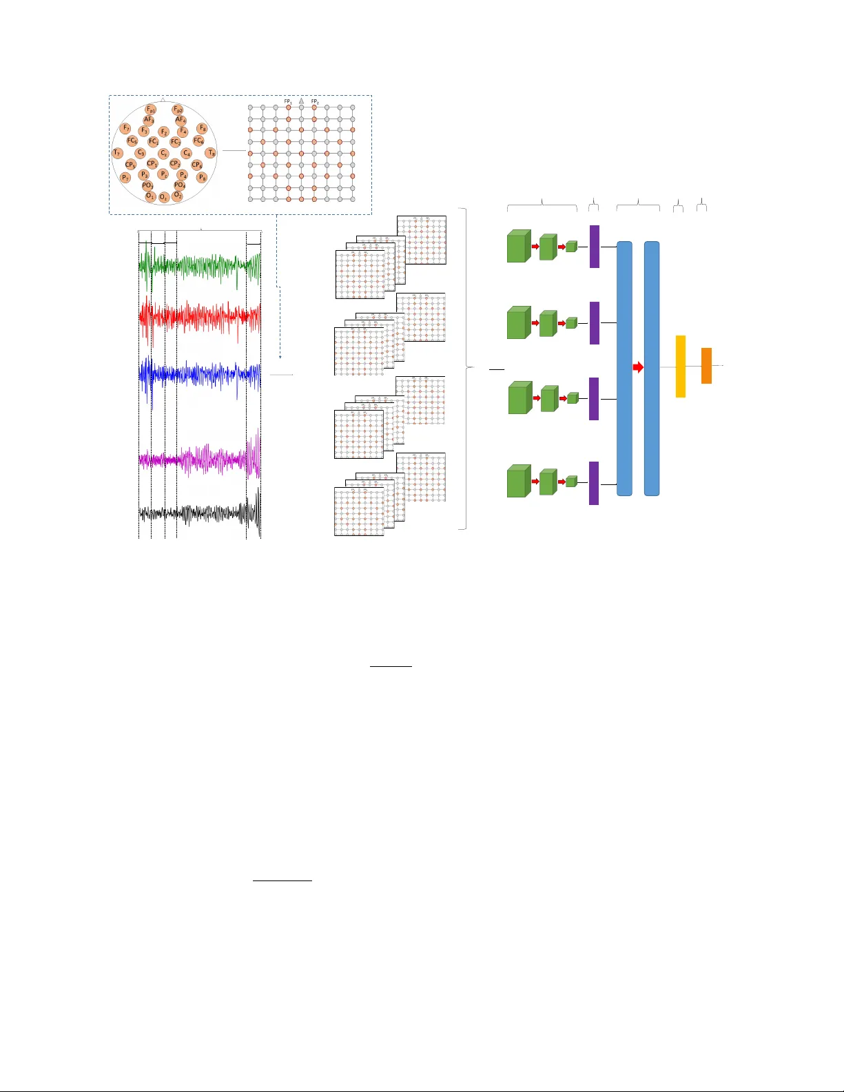
Authors: Theerawit Wilaiprasitporn, Apiwat Ditthapron, Karis Matchaparn
JOURNAL OF L A T E X CLASS FILES, VOL. 14, NO. 8, A UGUST 2015 1 Af fecti v e EEG-Based Person Identification Using the Deep Learning Approach Theerawit W ilaiprasitporn, Apiwat Ditthapron, Karis Matchaparn, T anaboon T ongb uasirilai, Nannapas Banluesombatkul and Ekapol Chuangsuwanich Abstract —Electroencephalograph y (EEG) is another mode f or performing P erson Identification (PI). Due to the nature of the EEG signals, EEG-based PI is typically done while the person is perf orming some kind of mental task, such as motor contr ol. Howev er , few works have considered EEG-based PI while the person is in different mental states (affecti ve EEG). The aim of this paper is to improv e the perf ormance of affective EEG- based PI using a deep lear ning approach. W e pr oposed a cascade of deep learning using a combination of Conv olutional Neural Networks (CNNs) and Recurr ent Neural Netw orks (RNNs) . CNNs are used to handle the spatial inf ormation fr om the EEG while RNNs extract the temporal inf ormation. W e ev aluated two types of RNNs, namely , Long Short-T erm Memory (CNN-LSTM) and Gated Recurrent Unit (CNN-GRU). The proposed method is evaluated on the state-of-the-art affective dataset DEAP . The results indicate that CNN-GR U and CNN-LSTM can perform PI from differ ent affective states and reach up to 99.90–100% mean Correct Recognition Rate (CRR), significantly outperforming a support vector machine (SVM) baseline system that uses power spectral density (PSD) features. Notably , the 100% mean CRR comes from only 40 subjects in DEAP dataset. T o reduce the number of EEG electrodes from thirty-two to five for more practical applications, the frontal region gives the best results reaching up to 99.17% CRR (fr om CNN-GR U). Amongst the two deep learning models, we find CNN-GR U to slightly outperform CNN-LSTM, while having faster training time. Furthermore, CNN-GR U overcomes the influence of affective states in EEG- Based PI reported in the previous works. Index T erms —Electroencephalography , P ersonal identification, Biometrics, Deep lear ning, Affecti ve computing, Con volutional neural networks, Long short-term memory , Recurrent neural networks I . I N T RO D U C T I O N I N today's world of lar ge and complex data-driven ap- plications, research engineers are inspired to incorporate multiple layers of artificial neural networks or deep learning (DL) techniques into health informatic-related studies such as bioinformatics, medical imaging, pervasi ve sensing, medical informatics and public health [1]. Such studies also include This work was supported by The Thailand Research Fund under Grant MRG6180028. T . W ilaiprasitporn and N. Banluesombatkul are with Bio-inspired Robotics and Neural Engineering Lab, School of Information Science and T echnology , V idyasirimedhi Institute of Science & Engineering, Rayong, Thailand (e-mail: theerawit.w@vistec.ac.th). A. Ditthapron is with the Computer Department, W orcester Polytechnic Institute, W orcester, MA, USA. K. Matchaparn is with the Computer Engineering Department, King Mongkut’ s University of T echnology Thonb uri, Bangkok, Thailand. T . T ongbuasirilai is with Department of Science and T echnology , Link ¨ oping Univ ersity , Sweden E. Chuangsuw anich is with the Computer Engineering Department, Chula- longkorn Univ ersity , Bangkok, Thailand. those relating to frontier neural engineering research into brain activity using the non-inv asi ve measurement technique called electroencephalography (EEG). The fundamental con- cept of EEG in volves measuring electrical activity (v ariation of v oltages) across the scalp. The EEG signal is one of the most complex in health data and can benefit from DL techniques in v arious applications such as insomnia diagnosis, seizure detection, sleep studies, emotion recognition, and Brain-Computer Interface (BCI) [2]–[7]. Howe ver , EEG-based Person Identification (PI) research using DL is scarcely found in literature. Thus, we are moti vated to work in this direction. EEG-based PI is a biometric PI system–fingerprints, iris, and face for example. EEG signals are determined by a person’ s unique pattern and influenced by mood, stress, and mental state [8]. EEG-based PI has the potential to protect encrypted data under threat. Unlike other biometrics, EEG signals are dif ficult to collect surreptitiously , since the y are concealed within the brain [9]. Besides the person’ s unique pattern, a passcode or pin can also be recognized from the same signal, while ha ving a lo w chance of being eav esdropped. EEG signals also lea ve no heat signal or fingerprint behind after use. The PI process shares certain similarities with the person verification process, but their purposes are different. Person verification validates the biometrics to confirm a person’ s identity (one-to-one matching), while PI uses biometrics to search for an identity match (one-to-many matching) on the database [10]. EEG-based PI system dev elopment has dramat- ically increased in recent years [11], [12]. Motor tasks (eye closing [13], hands movement [14], etc.), visual stimulation [15]–[17] and multiple mental tasks such as mathematical calculation, writing text, and imagining movements ( [18]) are three major tasks in stimulating brain responses for EEG- based PI [19]. T o identify a person, it is very important to in vestigate the stimulating tasks which can induce personal brain response patterns. Moods, feelings, and attitudes are usually related to personal mental states which react to the en vironment. Howe ver , emotion-elicited EEG has been rarely in vestigated to perform person identification. There are several reports on affecti ve EEG-based PI; one with a small affecti ve dataset [20], one reaching less than a 90% mean Correct Recognition Rate (CRR) [21] and another using the same dataset as our w orks with PSD-based feaures reached up to 97.97% mean CRR. Thus, the aim of this paper is to ev aluate the usability of EEG from elicited emotions for person identification applications. The study of affecti ve EEG- based PI can help us gain a greater understanding concerning JOURNAL OF L A T E X CLASS FILES, VOL. 14, NO. 8, A UGUST 2015 2 the performance of personal identification among different affecti ve states. This study mainly focuses on the state-of-the- art EEG dataset for emotion analysis named DEAP [22]. A recent critical survey on the usability of EEG-based PI resulted in se veral major signal processing techniques to help perform feature extraction and classification [12]. Power Spectral Density (PSD) methods [23]–[26], the Autoregressiv e Model (AR) [27]–[32], W av elet T ransform (WT) [33], [34] and Hilbert-Huang T ransform (HHT) [35], [36] are useful for feature extraction. For feature classification, k-Nearest Neighbour (k-NN) algorithms [37], [38], Linear Discriminant Analysis (LD A) [39], [40], Artificial Neural Networks (ANNs) with a single hidden layer [23], [41]–[43] and kernel methods [44], [45] are popular techniques. In this study , we propose a DL technique to perform both the feature extraction and classification tasks. The proposed DL model is a cascade of the CNN and GR U. CNN and GR U are supposed to capture spatial and temporal information from EEG signals, respectively . A similar cascade model based on CNN and LSTM has recently been applied in a motor imagery EEG classification aiming at BCI applications, howe ver , they did not study GR Us to perform this task [5]. The main contribution of this in vestigation can be summa- rized as follows: • W e propose an effecti ve EEG-based PI using a DL approach, which has not been in vestigated previously to any extent. • The proposed approach overcomes the influence of af fec- tiv e states in using EEG for PI task. • Using our proposed technique, we in vestigate whether any EEG frequency bands outperform others to perform affect EEG-based PI task. • W e performed e xtensiv e e xperimental studies using a set of fiv e EEG electrodes from different scalp areas. Specifically , these studies reports the feasibility of the proposed technique to handle real world scenarios. • W e provide the performance comparison of the proposed cascade model (CNN-GR U) against a spatiotemporal DL model (CNN-LSTM), and other systems proposed in literature [21], [46]. In summary , the experimental results guarantee that the CNN- GR U con ver ges faster than CNN-LSTM while ha ving a slightly higher mean CRR, especially when using a small amount of electrode. Furthermore, CNN-GRU ov ercomes the influence of affecti ve states in EEG-Based PI reported in the previous works [46], [47]. The structure of this paper is as follows. Sections II and III present the background and methodology , respecti vely . The results are reported in Section IV . Section V discusses the results from the e xperimental studies. Moreo ver , the beneficial points are highlighted for comparison over previous w orks for further inv estigation. Finally , the conclusion is presented in Section VI. I I . T H E D E E P L E A R N I N G A P P RO AC H T O E E G There has been a surge of deep learning-related methods for classification of EEG signals in recent years. Since EEG signals are recordings of biopotentials across the scalp o ver time, researchers tend to use DL architectures for capturing both spatial and temporal information. A cascade of CNN, followed by an RNN, often an LSTM, is typically used. These cascade architectures work according to the nature of neural networks, where the proceeding layers function as feature extractors for the latter layers. CNN are often used as the initial layers of deep learning architectures in order to e xtract meaningful patterns or fea- tures. The key element of CNN is the con v olution operation using small filter patches (kernels). These filters are able to automatically learn local patterns which can be combined to- gether to form more complex features when stacking multiple CNN layers together . Within the stack of con volution layers, pooling layers are often placed intermittently . The pooling layers subsample the output of the con volution layers by outputting only the maximum value for each small region. The subsampling allows the con volution layer after the pooling layer to work on a different scale than the layers before it. These features learned from the CNN can be used as input to other network structures to perform sophisticated tasks such as object detection or semantic segmentation [48]. For EEG signals, it makes sense to feed the local structures learned by the CNN to LSTMs, which can better handle temporal information. Zhang et al. also tried a 3D CNN to exploit the spatiotemporal information directly within a single layer . Howe ver , the results were slightly behind a cascade of the CNN-LSTM model [5]. This might be due to the fact that LSTMs are often better at handling temporal information since they can choose to remember and discard information depending on the context. Another type of recurrent neural network called the Gated Recurrent Unit (GR U) has also been proposed as an alternative to the LSTM [49]. The GR U can be considered as a simplified version of the LSTM. GR Us have two gates (reset and update) instead of three gates as in the LSTMs. GR Us directly output the captured memory , while LSTMs can choose not to output its content due to the output gate. Figure 1 (a) shows the interconnections of a GR U unit. Just as a fully connected layer is composed of multiple neurons, a GR U layer is composed of multiple GR U units. Let x t be the input at time step t to a GR U layer . The output of the GR U layer , h t , is a vector composing the output of each individual unit h j t , where j is the index of the GRU cell. The output activ ation is a linear interpolation between the acti v ation from the pre vious time step and a candidate activ ation, ˆ h j t . h j t = (1 − z j t ) h j t − 1 + z j t ˆ h j t (1) where an update g ate, z j t , decides the interpolation weight. The update gate is computed by z j t = F j ( W z x t + U z h t − 1 ) (2) where W z and U z are trainable weight matrices for the update gate, and F j () takes the j -th index and pass it through a non- linear function (often a sigmoid). The candidate activ ation is JOURNAL OF L A T E X CLASS FILES, VOL. 14, NO. 8, A UGUST 2015 3 also controlled by an additional reset gate, r t , and computed as follows: ˆ h j t = G j ( W x t + U ( r t h t − 1 )) (3) where represents an element-wise multiplication, and G j () is often a tanh non-linearity . The reset gate is computed in a similar manner as the update gate: r j t = F j ( W r x t + U r h t − 1 ) (4) On the other hand, LSTMs hav e three gates, input, output, and forget gates which are denoted as i j t , o j t , f j t , respectiv ely . They also ha ve an additional memory component for each LSTM cell, c j t . A visualization of an LSTM unit is shown in Figure 1 (b). The gates are calculated in a similar manner as the GR U unit except for the additional term from the memory component. i j t = F j ( W i x t + U i h t − 1 + V i c t − 1 ) (5) o j t = F j ( W o x t + U o h t − 1 + V o c t ) (6) f j t = F j ( W f x t + U f h t − 1 + V j c t − 1 ) (7) where V i , V o , and V j are trainable diagonal matrices. This keeps the memory components internal within each LSTM unit. The memory component is updated by forgetting the exist- ing content and adding a new memory component ˆ c j t : c j t = f j t c j t − 1 + i j t ˆ c j t (8) where the new memory content can be computed by: ˆ c j t = G j ( W c x t + U c h t − 1 ) (9) Note how the updated equation for the memory component is gov erned by the forget and input gates. Finally , the output of the LSTM unit is computed from the memory modulated by the output gate according to the following equation: h j t = o j t tanh ( c j t ) (10) Previous works using deep learning with EEG signals hav e explored the use of CNN-LSTM cascades [5]. Howe ver , GR Us hav e been shown in many settings to often match or e ven beat LSTMs [50]–[52]. GR Us hav e the ability to perform better with a smaller amount of training data and are faster to train than LSTMs. Thus, in this work, CNN-GR U cascades are also explored and compared against the CNN-LSTM in both accuracy and training speed. I I I . M E T H O D O L O G Y In this section, we first illustrate the DEAP affecti ve EEG dataset [22] that we used to conduct experimental studies and also describe the pre-processing step of our solution. Since DEAP was created for mental state classification purposes, we describe our data partition methodology used to make it more suitable to perform the PI task. Finally , we explain the proposed DL approach and its implementation. Input x Output h h ^ r z Previous output (a) GRU Input x Output h c ^ i Previous output Previous memory f c o (b) LSTM Fig. 1. Comparison between GR U and LSTM structures and their operations T ABLE I A FF EC T I V E E EG D AT A F O R M A T W IT H L A B E L Array Name Array Shape data 32 x 40 x 32 x 8064 participant x video/trial x EEG x data labels 32 x 40 x 2 participant x video/trial x (valence, arousal) A. Affective EEG Dataset In this study , we performed experiments using DEAP af- fectiv e EEG dataset which is considered as a standard dataset to perform emotion or affecti ve recognition tasks [53]. Thirty- two healthy participants participated in the experiment. They were asked to watch affecti ve elicited music videos and score subjectiv e ratings (v alence and arousal) for forty video clips during the EEG measurement. A summary of the dataset is giv en in T able I . The EEG dataset was pre-processed using the following steps: • The data was down-sampled to 128 Hz. • EOG artifacts were removed using the blind source sep- aration technique called independent component analysis (ICA). • A bandpass filter from 4.0–45.0 Hz w as applied to the original dataset. The signal was further filtered into different bands as follows: Theta (4–8 Hz), Alpha (8–15 Hz), Beta (15–32 Hz), Gamma (32–40 Hz), and all bands (4–40 Hz). • The data was averaged to a common reference. • The data was segmented into 60-second trials, and the 3-second pre-trial segments were removed. Most researchers hav e been using this dataset to de velop an affecti ve computing algorithm; howe ver , we used this affecti ve dataset for studying EEG-based PI. B. Subsampling and Cross V alidation Affecti ve EEG is categorised by the standard subjective measures of v alence and arousal scores (1–9), with 5 as the threshold for defining low (score < 5) and high (score ≥ 5) lev els for both valence and arousal. Thus, there were four affecti ve states in total, as stated in T able II. T o simulate practical PI applications, we randomly selected 5 EEG trials JOURNAL OF L A T E X CLASS FILES, VOL. 14, NO. 8, A UGUST 2015 4 T ABLE II N U MB E R O F P A RT IC I PAN T S I N EA CH S T A T E A F T E R S UB S A M PL I N G Affective States Number of Participants Low V alence, Lo w Arousal (LL) 26 Low V alence, High Arousal (LH) 24 High V alence, Low Arousal (HL) 23 High V alence, High Arousal (HH) 32 All States 32 per state per person (recorded EEG from 5 video clips) for the experiments. Thus, new users can spend just 5 minutes watching 5 videos for the first registration. T able II presents a number of subjects in each affecti ve state. The numbers were different in each state because some subjects had less than 5 recorded EEG trials categorized into the state. Furthermore, we aimed to identify a person from a short-length of EEG: 10-seconds. Each EEG trial in DEAP lasts long 60-seconds as a stimulus video. Thus, we simply cut one EEG trial into 6 subsamples. Finally , we had 30 subsamples (6 subsamples × 5 trials) from each participant in each of the affecti ve states. In summary , labels in our experiments (personal identifica- tion) are ID of participants. Data and labels that ha ve been used can be described as: • Data: number of participants × 30 subsamples × 1280 EEG data points (10-seconds with 128 Hz sampling rate) • Label: number of participants × 30 subsamples × 1(ID) In all experiments, the training, validation, and testing sets were obtained using stratified 10-fold cross-validation. As for the subsamples, 80% of them were used as training data. As for the validation and test sets, each of them contained 10% of the subsamples. In each fold, we make sure that the subsamples from each trial is not assigned to more than one set. That is, it can be either in the training, v alidation or test set. Thus, the subsamples in the training, the validation and the test sets were totally independent. C. Experiment I: Comparison of affective EEG-based PI among differ ent affective states Since datasets contains EEG from fiv e af fecti ve states as also shown in T able II, an experiment was carried out to ev aluate which affectiv e states would provide the highest CRR in EEG based PI applications. T o achie ve this goal, two approaches were implemented: deep learning and conv entional machine learning. EEG in the range of 4–40 Hz was used in this experiment. 1) Deep Learning Approac h: Figure 2 demonstrates the preparation of the 10-second EEG data before feeding into the DL model. In general, a single EEG channel is a one- dimensional (1D) time series. Howe ver , multiple EEG chan- nels can be mapped into time series of 2D mesh (similar to a 2D image). For each time step of the input, the data point from each EEG channel is arranged into one 2D mesh shape of 9 × 9. 2D mesh size is empirically selected according to the international standard of an electrode placements (10-20 system) with covering all 32 EEG channels. The mesh point (similar to the pixel) which is not allocated for EEG channel is assigned to zeros value throughout the sequences. The mean and variance for each mesh (32 channels) is normalised individually . In this study , a non-ov erlapping sliding window is used to separate the data into one-second chunks. Since the sampling rate of input data is 128 Hz, the windo w size is 128 points. Thus, for each 10-second EEG data, a 10 × 9 × 9 × 128- dimensional tensor is obtained. The deep learning model starts with three layers of 2D- CNN (applied to the mesh structure). Each mesh frame from the 128 windows is considered individually in the 2D-CNN. Since this is also a time series, the 2D-CNN is applied to each sliding window , one windo w at a time, but with shared parameters. This structure is called a TimeDistrib uted 2DCNN layer . After the TimeDistrib uted 2DCNN layers, a T imeDis- tributed Fully Connected (FC) layer is used for subsampling and feature transformation. T o capture the temporal structure, two recurrent layers (GR U or LSTM layers) are then applied along the dimension of the sliding windows. Finally , a FC layer is applied to the recurrent output at the final time step with a softmax function for person identification. The following specific model parameters are used in Exper- iments I–III. Three layers of T imeDistributed 2DCNNs with 3 × 3 kernels. W e set the number of filters to 128, 64 and 32 for the first, second and third layer respectively . ReLu nonlinearity is used. Batch normalization and dropout are applied after ev ery con volutional layer . For the recurrent layers, we used 2 layers with 32 and 16 recurrent units, respectiv ely . Recurrent dropout was also applied. The dropout rates in each part of the model were fixed at 0.3. W e used RMSprop optimizer with a learning rate of 0.003 and a batch size of 256. Although these parameters are held fixed, these settings were found to be good enough for our purposes. The effect of parameter tuning for DL models will be further explored in Experiment IV . 2) Con ventional Machine Learning Appr oach using Sup- port V ector Machine (SVM): The algorithm aims to locate the optimal decision boundaries for maximising the margin between two classes in the feature space [54]. This can be done by minimizing the loss: 1 2 w t w + C n X i =1 ξ i , (11) under the constraint y i ( w t φ ( x i ) + b ) ≥ 1 − ξ i and ξ i ≥ 0 , i = 1 , ..., n. (12) C is the capacity constant, w is the vector of coefficients, b is a bias offset, and y i represents the label of the i -th training example from the set of N training examples. The larger the C value, the more the error is penalized. The C value is optimized to avoid overfitting using the validation dataset described earlier . In the study of person identification, the class label repre- sents the identity number of the participant, considered as a multi-class classification problem. Numerous SVM algorithms can be used such as the “one-against-one” approach, “one-vs- the-rest” approach [54], or k-class SVM [55]. T o illustrate a strong baseline, the “one-against-one” approach, which re- quires higher computation, is chosen for its robustness tow ards JOURNAL OF L A T E X CLASS FILES, VOL. 14, NO. 8, A UGUST 2015 5 10 seconds . . . . . . Mapping scalp 2D mesh (shape = 9 x 9) F p1 F p2 AF 3 O z O 2 . . . . . . Output (person) 32 channels 1 st second 2 nd second 3 rd second 10 th second 1 st 2 nd 3 rd 10 th . . . shape = 9x9x128 time distributed 2D-CNN Mapping input shape = 10x9x9x128 FC stacks of GRU/ LSTM FC SoftMax . . . . . . . . . . . . . . . . . . . . . . . . . . . . . . . . Fig. 2. Implementation of the cascade CNN-GR U/LSTM model according to EEG data. Meshing is the first step in converting multi-channel EEG signals into sequences of 2D images. The 2D mesh time series is passed through the cascade of CNN and recurrent layers for training, validation, and testing. imbalanced classes and small amounts of data. The “one- against-one” SVM solves multi-class classification by building classifiers for all possible pairs of classes resulting in N ( N − 1) 2 classifiers. The predicted class label is the one most yielded from all classifiers. In this work, the W elch’ s method is employed as the feature extraction method for the SVM. It is a well-kno wn PSD estimation method, for reducing the variance in periodogram estimation by breaking the data into ov erlapped segments. Be- fore feeding into the SVM, a normalization step is performed. For normalization, Z-score scaling is adopted, because, exper - imentally , it performs better than other normalization methods such as min-max and unity normalization in EEG signal processing. x normal ized = x − ¯ x train s train (13) Normalization parameters, sample mean ( ¯ x train ) and sample standard deviation ( s train ) , are computed o ver the training set. The validation set is used to determine the best parameter C chosen from 0 . 01 , 0 . 1 , 1 , 10 . 100 for each experiment. Note: accor ding to the r esults fr om Experiment I (EX I), DL appr oaches perform perfectly even when using a mixtur e of affective state (all states). The affective states do not affect PI performance for DL models. Therefor e, the affective EEG states wer e not consider ed, and the all states setting is used in the remaining experiments. D. Experiment II: Comparison of af fective EEG-based PI among EEGs fr om differ ent frequency bands EEG is con ventionally used to measure variations in elec- trical acti vity across the human scalp. The electrical activity occurs from the oscillation of billions of neural cells inside the human brain. Most researchers usually di vided EEG into frequency bands for analysis. Here, we defined Theta (4–8 Hz), Alpha (8–15 Hz), Beta (15–32 Hz), Gamma (32–40 Hz) and all bands (4–40 Hz). T ypical Butterworth bandpass filter had incorporated to extract EEGs from different frequency bands. In this study , we question whether or not frequency bands affect PI performance. T o answer the question, we incorporate CNN-LSTM (stratified 10-fold cross-validation), CNN-GR U, and SVM (as performed in EX I) for CRR comparison. Note: accor ding to the results of Experiment II, all bands (4–40 Hz) pro vided the best CRR and we continued to use all bands for the remainder of the study . JOURNAL OF L A T E X CLASS FILES, VOL. 14, NO. 8, A UGUST 2015 6 O 2 F p1 F p2 AF 3 AF 4 F 3 F Z F 4 F 7 F 8 FC 5 FC 1 FC 2 FC 6 T 7 C 3 C z C 4 T 8 CP 5 CP 1 CP 6 CP 2 P z P 4 P 8 P 7 PO 3 PO 4 O 1 O z P 3 (a) Frontal (F) O 2 F p1 F p2 AF 3 AF 4 F 3 F Z F 4 F 7 F 8 FC 5 FC 1 FC 2 FC 6 T 7 C 3 C z C 4 T 8 CP 5 CP 1 CP 6 CP 2 P z P 4 P 8 P 7 PO 3 PO 4 O 1 O z P 3 (b) Central and P arietal (CP) O 2 F p1 F p2 AF 3 AF 4 F 3 F Z F 4 F 7 F 8 FC 5 FC 1 FC 2 FC 6 T 7 C 3 C z C 4 T 8 CP 5 CP 1 CP 6 CP 2 P z P 4 P 8 P 7 PO 3 PO 4 O 1 O z P 3 (c) T emporal (T) O 2 F p1 F p2 AF 3 AF 4 F 3 F Z F 4 F 7 F 8 FC 5 FC 1 FC 2 FC 6 T 7 C 3 C z C 4 T 8 CP 5 CP 1 CP 6 CP 2 P z P 4 P 8 P 7 PO 3 PO 4 O 1 O z P 3 (d) Occipital and P arietal (OP) O 2 F p1 F p2 AF 3 AF 4 F 3 F Z F 4 F 7 F 8 FC 5 FC 1 FC 2 FC 6 T 7 C 3 C z C 4 T 8 CP 5 CP 1 CP 6 CP 2 P z P 4 P 8 P 7 PO 3 PO 4 O 1 O z P 3 (e) Frontal and P arietal (FP) Fig. 3. Experimental Study III evaluates the CRR of the EEG-based PI in different sets of sparse EEG electrodes. Fiv e EEG electrode channels from each part of the scalp were grouped into fi ve different configurations (a-e) T ABLE III V A R I A T I ON I N T H E N UM B E R O F FI LT ER S FO R EA CH C NN L A Y ER S WH I L E FI X IN G TH E NU M B ER O F G RU / LS T M U N I T S CNN GRU/LSTM 128 32. 16 128, 64 32, 16 128, 64, 32 32, 16 E. Experiment III: Comparison of affective EEG-based PI among EEGs fr om sets of sparse EEG electr odes In this experiment, we hypothesized whether or not the number of electrodes could be reduced from thirty-two chan- nels to fiv e while maintaining an acceptable CRR . The lower the number of electrodes required, the more user -friendly and practical the system. T o in vestigate this question, we defined sets of fi ve EEG electrodes as sho wn in Figure 3, including Frontal (F) Figure 3(a), Central and Parietal (CP) Figure 3(b), T emporal (T) Figure 3(c), Occipital and Parietal (OP) Figure 3(d), and Frontal and Parietal (FP) Figure 3(e). According to EX I and II, the DL approach significantly outperforms the traditional SVM in PI applications. Thus, we incorporated only CNN-GR U and CNN-LSTM in this in vestigation. T ABLE IV V A R I A T I ON I N T H E N UM B E R O F G RU / L S TM U NI T S W H I LE FI XI N G T H E C N N L AYE R S CNN GRU/LSTM 128, 64, 32 16, 8 128, 64, 32 32, 16 128, 64, 32 64, 32 F . Experiment IV : Comparison of pr oposed CNN-GR U against CNN-LSTM and other r elevant approac hes towar ds affective EEG-based PI application First, we ev aluated our proposed CNN-GR U against a spa- tiotemporal DL model, namely which CNN-LSTM [5]. Both approaches have been previously described in detail in Section III and Figure 2. In this study , we measured the performance in terms of the mean CRR and the con vergence speed as we tuned the size of the models by varying the number of CNN layers and the number of GR U/LSTM units. W e also compared our best models against other con ventional machine learning methods and rele vant works, such as Mahalanobis distance- based classifiers, using either PSD or spectral coherence (COH) as features (reproduced from [25]) and DNN/SVM as proposed in [21]. 1) Deep Learning Appr oach: T o find suitable CNN layers for cascading with either GRU or LSTM, the numbers of CNN layers were varied as presented in T able III. The selected CNN layers were then cascaded to GR U/LSTM and the numbers of GR U and LSTM units varied, as can be seen in T able IV. 2) Baseline Appr oach: As previously mentioned, the Ma- halanobis distance-based classifier with either PSD or COH as features was used as a baseline. This approach was reported to provide the highest CRR among multiple approaches in a recent critical revie w paper on EEG-based PI [12]. Howe ver , it has never been applied on the DEAP affecti ve datasets. T o obtain the PSD and COH features, the same parameters were used as reported in [25], except that the number of FFT points was set to 128. Each PSD feature has N P S D = 32 elements (electrodes) and each COH feature has N C OH = 496 elements (pairs). Classification w as then performed on the transformed features. Fisher’ s Z transformation was applied to the COH features and a logarithmic function to the PSD features. After the transformed PSD and COH features for each element were obtained, the Mahalanobis distances, d m,n , were then computed as shown in Equation 14. d m,n = ( O m − µ n )Σ − 1 ( O m − µ n ) T (14) where O m is the observed feature vector , µ n is the mean feature vector of class n , and Σ − 1 is the inv erse pooled co- variance matrix. The pooled co variance matrix is the a veraged- unbiased cov ariance matrix of all class distributions. For each sample, the Mahalanobis distances were computed between the observed sample m and the class distribution n, thus a distance vector of size N where N = 32, representing the number of classes (participants) in the dataset. T wo different schemes were used in [25]. The first scheme was a single-element classification to perform the identifi- cation of each electrode separately . The other scheme was JOURNAL OF L A T E X CLASS FILES, VOL. 14, NO. 8, A UGUST 2015 7 T ABLE V C O MPA R IS O N O F TH E M E A N C O R RE C T R E C O GN I T IO N RAT E O R CRR ( W I T H S T A N DA R D E R RO R BA R ) A M O N G D I FFE R E NT A FFE C T I VE S T A T E S A N D D I FFE R E N T R EC O G N IS E D A P P ROA CH E S . C N N -G RU A ND C NN - L S TM S I GN I FI C AN T L Y OU T P E RF O R M ED TH E TR A D I TI O NA L SV M IN E VE RY A FF EC T I V E S T A T E ( I N C LU D I N G A L L S T ATE S ) , * N O TE S p < 0.01 . E E G I N T H E R A NG E O F 4– 4 0 H Z HA S BE E N U S E D I N T H I S E X PE R I M EN T . Mean CRR [%] States CNN-GRU CNN-LSTM SVM LL 99.90 ± 0.10* 99.79 ± 0.14* 33.02 ± 1.58 LH 99.71 ± 0.19* 100.0* 36.38 ± 1.71 HL 99.86 ± 0.14* 99.86 ± 0.14* 36.25 ± 2.45 HH 99.87 ± 0.12* 99.74 ± 0.26* 33.59 ± 1.65 All States 100.0* 99.79 ± 0.14* 33.02 ± 1.58 the all-element classification, combining the best subset of electrodes using match score fusion. W e chose the all-element classification scheme which yielded better performance. W e modified the scheme to be compatible to this w ork by selecting all electrodes instead of choosing just a subset. Stratified 10- fold cross-validation was also performed on the all-element classification to obtain the mean CRR . I V . R E S U L T S Experimental results are reported separately in each study . Then all of them are summarized at the end of the section. A. Results I: comparison of af fective EEG-based PI among differ ent affective states The comparison of the mean correct recognition rate or CRR (with standard error bar) among different affecti ve states and dif ferent recognized approaches had been shown in T a- ble V. Statistical testing named one way repeated measures ANO V A (no violation on Sphericity Assumed) with Bon- ferroni pairwise comparison (post-hoc comparison) had been implemented for comparison of mean CRR (stratified 10-fold cross-validation). In the comparison of CRR among different affecti ve states, the statistical results demonstrate that the EEG (4–40 Hz) fr om dif fer ent affective states does not affect the perfor- mance of affective EEG-based PI in all reco gnised appr oaches (F(4)=0.805, p = 0.530 , F(4)=0.762, p = 0.557 and F(4)=0.930, p = 0.457 for CNN-GR U, CNN-LSTM, and SVM, respec- tiv ely). Moreov er , in comparison of CRR among dif ferent ap- proaches, the statistical results show a significant difference in the mean CRR among CNN-GRU, CNN-LSTM, and SVM approaches. In pairwise comparison, CNN-GRU and CNN- LSTM significantly outperformed the traditional SVM in e very affecti ve state (including all states), p < 0.01 . Both CNN-GR U (in all states) and CNN-LSTM (in LH) reached up to 100% in mean CRR . Further reports on comparative studies of CNN- GR U and CNN-LSTM for EEG-based PI against previous works can be seen in Results IV . B. Results II: comparison of af fective EEG-based PI among EEGs fr om differ ent fr equency bands Here, we report the comparison of the mean correct recog- nition rate or CRR among dif ferent EEG frequency bands and T ABLE VI C O MPA R IS O N O F TH E M E A N C O R RE C T R E C O GN I T IO N RAT E O R C R R ( W IT H STA N DA RD E RR OR BA R ) A M O NG D IFF E R EN T EE G FR E Q UE N C Y BA N D S A N D D I FFE R E N T R E CO G N IS E D A P P ROA C HE S , N O D I FF E RE N C E S I N C N N- G RU , C N N - LS T M , A N D S V M W E R E F O U ND I N L OW FR E Q UE N C Y BA N D S ( T HE TA ( 4 – 8 H Z ) A N D A L P H A ( 8 –1 5 H Z ) ) . H OW E V ER , TH E Y S I GN I FI C AN T L Y OU T P E RF O R M ED TH E SV M IN B ETA ( 1 5 – 32 H Z ) , G A MM A (3 2 – 4 0 H Z ) , A N D A L L BA N D S ( 4 – 40 H Z ) , * N OT E S p < 0.01 . Mean CRR [%] CNN-GRU CNN-LSTM SVM 4-8 Hz 99.69 ± 0.22 99.69 ± 0.22 98.54 ± 0.35 8-15 Hz 99.58 ± 0.23 99.69 ± 0.22 98.75 ± 0.34 15-32 Hz 99.90 ± 0.10* 99.86 ± 0.16* 87.50 ± 0.64 32-40 Hz 100.0* 99.74 ± 0.14* 33.54 ± 1.57 all bands 100.0* 99.79 ± 0.14* 33.02 ± 1.58 different recognized approaches (shown in T able VI) using the same statistical testing as same as in Section IV A). In the comparison of CRR among different frequency bands, the statistical results demonstrate that EEG fr om dif ferent fr equency bands does not affect the performance of affective EEG-based PI in CNN-GR U and CNN-LSTM appr oaches ( F(4)=2.168, p = 0.092 and F(4)=0.144, p = 0.964 for CNN- GR U and CNN-LSTM, respectiv ely). Ho wev er , the SVM approach shows that Theta (4–8 Hz) and Alpha (8–15 Hz) pro- vide significantly higher CRR than Beta (15–32 Hz), Gamma (32–40 Hz), and all bands (4–40 Hz) ( F(4)=1309.747, p < 0.01 in ANO V A testing and p < 0.01 in all pairwise comparisons). Furthermore, in the comparison of CRR among different approaches, there were no differences in CNN-GRU, CNN- LSTM, and SVM for low frequency bands (Theta (4–8 Hz) and Alpha (8–15 Hz)). Ho wev er , CNN-GRU and CNN-LSTM significantly outperformed the SVM in Beta (15–32 Hz), Gamma (32–40 Hz), and all bands (4–40 Hz), p < 0.01 . CNN- GR U and CNN-LSTM reached up to 100% and 99.79%, respectiv ely , in all bands. C. Results III: Comparison of affective EEG-based PI among EEGs fr om sets of sparse EEG electr odes According to Figure 4, one-way repeated measures ANO V A with Bonferroni pairwise comparison (post-hoc) reported that fiv e electrodes in the F set provided a significantly higher mean CRR than the other sets in both CNN-GR U and CNN- LSTM p < 0.05 . CNN-GR U and CNN-LSTM reached up to (99.17 ± 0.34%) and (98.23 ± 0.52%) mean CRR , respectiv ely (stratified 10-fold cross-v alidation). T o reduce the number of EEG electrodes from thirty-two to five for more practical application, F 3 , F 4 , F z , F 7 and F 8 were the best fi ve electrodes for application in similar scenarios to this experiment. D. Results IV : Comparison of pr oposed CNN-GR U against CNN-LSTM and the other r elevant appr oaches towar ds affec- tive EEG-based PI application T able VII and T able VIII present mean CRR (stratified 10- fold cross-validation) from the proposed CNN-GRU against the conv entional spatiotemporal DL model, namely CNN- LSTM, in various parameter settings (number of CNN layers and GRU/LSTM units). Mean CRR s from CNN-GR U were JOURNAL OF L A T E X CLASS FILES, VOL. 14, NO. 8, A UGUST 2015 8 Mean CRR 0% 25% 50% 75% 100% GRU LSTM F CP T OP FP * - - * Fig. 4. Comparison of CRR among five sets of electrodes. The frontal part (F) provided significantly higher CRR compared to the others p < 0.05 . On the other hand, occipital and parietal (OP) provided significantly lower CRR compared to the others p < 0.05 . T ABLE VII C O MPA R IS O N O F M E A N CRR R E SU LT S B E TW E E N D I FFE R E NT C NN LAY ER S W I TH 3 2 E E G E L E C TR OD E S Mean CRR [%] CNN GRU/LSTM GRU LSTM 128 32, 16 100 ± 0.00 99.69 ± 0.16 128, 64 32, 16 99.90 ± 0.10 99.69 ± 0.16 128, 64, 32 32, 16 99.90 ± 0.10 99.90 ± 0.10 higher or equal compared to those from CNN-LSTM in all settings. The standard t-test indicated that the mean CRR from CNN-GR U was significantly higher ( p < 0.01 ) than that of the CNN-LSTM in 3 CNN layers with 128, 64, and 32 filters and 2 layers of GR U/LSTM with 16 and 8 units. In the comparison of training speed between the two approaches, CNN layers were fixed with 128, 64, 32 filters because the mean CRR was equal as shown in T able VII. Figure 5 and Figure 6 present a training speed comparison (in terms of training loss by epoch) from CNN-GR U and CNN-LSTM on 2 layers of GRU/LSTM with 16, 8 and 32, 16 units, respecti vely . It was obvious that training loss from CNN-GR U was decreasing faster than from CNN-LSTM. These results were also consistent with GR U/LSTM for 64, 32 units. T able IX demonstrates EEG-based PI performance using the proposed approach (CNN-GRU) against conv entional DL (CNN-LSTM) and the baseline approach. The baseline ap- proaches are reproducing Mahalanobis distance-based classi- fier using PSD/COH as features and typical non-linear clas- sifiers (DNN or ANN or SVM) from previous works [21], [46], with the same datasets. CNN-GRU/LSTM (constructed using CNN layers with 128, 64, 32 filters and 2 layers of GR U/LSTM with 32 and 16 units) produced a higher mean CRR than the others. Furthermore, the CNN-GRU was better than CNN-LSTM both in terms of training speed (as shown Figure 5) and mean CRR with a small number of electrodes (fiv e from the frontal area). Tr ai n in g l o s s 0 1 2 3 4 Epoch 1 31 61 91 121 151 181 CNN-GRU CNN-LSTM th Fig. 5. Comparison of training loss by epoch between CNN-GR U and CNN- LSTM. The configuration consists of 3 CNN layers with 128, 64, 32 filters and 2 layers of GR U/LSTM with 16 and 8 units. Tr ai n in g l o s s 0 1 2 3 4 Epoch 1 21 41 61 81 101 121 141 161 181 CNN-GRU CNN-LSTM th Fig. 6. Comparison of training loss by epoch between CNN-GR U and CNN- LSTM. The configuration consists of 3 CNN layers with 128, 64, 32 filters and 2 layers of GR U/LSTM with 32 and 16 units. V . D I S C U S S I O N From the experimental results, we will focus on two kinds of issues, namely physical and algorithmic issues for af fecti ve EEG-based PI applications. The physical issues refer to the EEG capturing such as the dif ferent affecti ve states, the frequency bands, and the electrode positions on the scalp. The algorithmic issues were about how to use the proposed approach (CNN-GR U) on EEG in an effecti ve way for PI applications and the advantages of CNN-GR U ov er the other T ABLE VIII C O MPA R IS O N O F ME A N CRR R E S ULT S B E T WE E N D I FF ER E N T G RU / L ST M U N IT S WI T H 3 2 EE G EL E C TR O DE S . * DE N OT E S T H A T T H E M E A N CRR I S S I GN I FI C AN T L Y HI G H E R , p < 0.01 . Mean CRR [%] CNN GRU/LSTM GRU LSTM 128, 64, 32 16, 8 97.29 ± 0.75 * 89.58 ± 1.81 128, 64, 32 32, 16 99.90 ± 0.10 99.90 ± 0.10 128, 64, 32 64, 32 99.90 ± 0.10 99.79 ± 0.25 JOURNAL OF L A T E X CLASS FILES, VOL. 14, NO. 8, A UGUST 2015 9 T ABLE IX C O MPA R IS O N O F ME A N CRR W I T H P RO P OS E D D L AP P RO AC H ( C NN - G RU ) , C O N V EN T I ON A L D L A P P ROAC H CN N - L ST M , C O NV E N T IO NA L MA C HI N E L E A RN I N G A N D P R E VI O U S W O RK S O N TH E S A ME DA TA SE T S . Appr oach Numbers of Electrodes Mean CRR [%] CNN-GR U 32 99.90 ± 0.11 CNN-GR U 5 99.10 ± 0.34 CNN-LSTM 32 99.90 ± 0.11 CNN-LSTM 5 98.23 ± 0.52 Mahalanobis-PSD 32 47.09 ± 2.34 Mahalanobis-COH 32 47.81 ± 3.29 DNN [21] 8 85.0 ± 4.0 SVM [21] 8 88.0 ± 4.0 SVM or ANN-PSD [46] 32 97.97 relev ant approaches. Regarding the physical issues, the experimental results indicate that DL approaches (CNN-GR U and CNN-LSTM) can deal with EEG (4–40 Hz) from different affecti ve states (valence and arousal lev els), reaching up to 100% mean CRR . On the other hand, a traditional machine learning approach such as SVM using PSD as features did not reach 50% mean CRR . Howe ver , the SVM approach was found to improve considerably when focusing on specific EEG frequency bands, namely Theta (4–8 Hz) and Alpha (8–15 Hz). The SVM reached up to 98% mean CRR with either Theta or Alpha EEG. As for CNN-GRU and CNN-LSTM, EEG frequency bands had little to no ef fect because that the DL approaches can capture v arious hidden features (including non-frequency re- lated features). Thus the hidden features can still maintain high percentages of CRR T o reduce the number of EEG electrodes from thirty-two to five for more practical applications, F 3 , F 4 , F z , F 7 and F 8 were the best fiv e electrodes. CNN-GRU and CNN-LSTM reached up to 99.17% and 98.23% mean CRR , respectiv ely . The results show that EEG electrodes from the frontal scalp provided higher mean CRR than other positions on the scalp, which is consistent with previous w ork on EEG- based PI [25]. Concerning the algorithmic issue, the proposed CNN-GRU and conv entional spatiotemporal DL models (CNN-LSTM) for EEG-based PI outperformed the state-of-the-art and rel- ev ant algorithms (Mahalanobis distance-based classifier using PSD/COH as features, DNN, and SVM [25] [21]) on the same dataset. In the comparison between CNN-GR U and CNN- LSTM, CNN-GRU was obviously better in terms of training speed while having a slightly higher mean CRR , especially in when using a small amount of electrode. Furthermore, CNN- GR U ov ercomes the influence of af fectiv e states in EEG-Based PI reported in the previous works [46], [47]. V I . C O N C L U S I O N In conclusion, we e xplored the feasibility of using af fectiv e EEG for person identification. W e proposed a DL approach called CNN-GR U, as the classification algorithm. EEG-based PI using CNN-GR U reached up to 99.90–100% mean CRR with 32 electrodes, and 99.17% with 5 electrodes. CNN-GRU significantly outperformed the state-of-the-art and relev ant al- gorithms in our experiments. In the comparison between CNN- GR U and the conv entional DL cascade model (CNN-LSTM), CNN-GR U was obviously better in terms of training speed. The mean CRR from CNN-GR U was slightly higher than from CNN-LSTM, especially when using only five electrodes. Furthermore, CNN-GRU ov ercomes the influence of affecti ve states in EEG-Based PI reported in the previous works. R E F E R E N C E S [1] D. Rav ` ı, C. W ong, F . Deligianni, M. Berthelot, J. Andreu-Perez, B. Lo, and G.-Z. Y ang, “Deep learning for health informatics, ” IEEE journal of biomedical and health informatics , vol. 21, no. 1, pp. 4–21, 2017. [2] F . Movahedi, J. L. Coyle, and E. Sejdi ´ c, “Deep belief networks for electroencephalography: A revie w of recent contributions and future outlooks, ” IEEE Journal of Biomedical and Health Informatics , vol. PP , no. 99, p. 1, 2017. [3] M. Shahin, B. Ahmed, S. T . B. Hamida, F . L. Mulaf fer, M. Glos, and T . Penzel, “Deep learning and insomnia: Assisting clinicians with their diagnosis, ” IEEE Journal of Biomedical and Health Informatics , vol. 21, no. 6, pp. 1546–1553, Nov . 2017. [4] N. Lu, T . Li, X. Ren, and H. Miao, “ A deep learning scheme for motor imagery classification based on restricted boltzmann machines, ” IEEE T ransactions on Neur al Systems and Rehabilitation Engineering , v ol. 25, no. 6, pp. 566–576, Jun. 2017. [5] D. Zhang, L. Y ao, X. Zhang, S. W ang, W . Chen, and R. Boots, “EEG- based intention recognition from spatio-temporal representations via cascade and parallel conv olutional recurrent neural networks, ” arXiv pr eprint , vol. arXiv:1708.06578, 2017. [6] Y . R. T abar and U. Halici, “ A novel deep learning approach for classi- fication of EEG motor imagery signals, ” J ournal of neur al engineering , vol. 14, no. 1, p. 016003, 2016. [7] R. T . Schirrmeister, J. T . Springenberg, L. D. J. Fiederer , M. Glasstetter , K. Eggensperger , M. T angermann, F . Hutter , W . Burgard, and T . Ball, “Deep learning with convolutional neural networks for EEG decoding and visualization, ” Human brain mapping , vol. 38, no. 11, pp. 5391– 5420, 2017. [8] Q. Gui, Z. Jin, and W . Xu, “Exploring eeg-based biometrics for user identification and authentication, ” in 2014 IEEE Signal Pr ocessing in Medicine and Biology Symposium (SPMB) , Dec 2014, pp. 1–6. [9] E. Maiorana, D. L. Rocca, and P . Campisi, “On the permanence of eeg signals for biometric recognition, ” IEEE T ransactions on Information F or ensics and Security , vol. 11, no. 1, pp. 163–175, Jan 2016. [10] J. R. V acca, Biometric technologies and verification systems . Elsevier , 2007. [11] P . Campisi and D. L. Rocca, “Brain wav es for automatic biometric- based user recognition, ” IEEE Tr ansactions on Information F orensics and Security , vol. 9, no. 5, pp. 782–800, May 2014. [12] S. Y ang and F . Deravi, “On the usability of electroencephalographic signals for biometric recognition: A survey , ” IEEE T ransactions on Human-Machine Systems , vol. 47, no. 6, pp. 958–969, Dec. 2017. [13] L. Ma, J. W . Minett, T . Blu, and W . S. W ang, “Resting state eeg- based biometrics for individual identification using conv olutional neural networks, ” in 2015 37th Annual International Conference of the IEEE Engineering in Medicine and Biology Society (EMBC) , Aug 2015, pp. 2848–2851. [14] V . Patel, M. Burns, R. Chandramouli, and R. V injamuri, “Biometrics based on hand synergies and their neural representations, ” IEEE Access , vol. 5, pp. 13 422–13 429, 2017. [15] B. K. Min, H. I. Suk, M. H. Ahn, M. H. Lee, and S. W . Lee, “Individual identification using cognitiv e electroencephalographic neurodynamics, ” IEEE T ransactions on Information F orensics and Security , vol. 12, no. 9, pp. 2159–2167, Sep. 2017. [16] Y . Chen, A. D. Atnafu, I. Schlattner, W . T . W eldtsadik, M.-C. Roh, H. J. Kim, S.-W . Lee, B. Blankertz, and S. Fazli, “ A high-security EEG-based login system with RSVP stimuli and dry electrodes, ” IEEE T ransactions on Information F orensics and Security , v ol. 11, no. 12, pp. 2635–2647, 2016. [17] R. Das, E. Maiorana, and P . Campisi, “Visually ev oked potential for eeg biometrics using conv olutional neural netw ork, ” in 2017 25th Eur opean Signal Pr ocessing Confer ence (EUSIPCO) , Aug 2017, pp. 951–955. [18] R. das, E. Maiorana, and P . Campisi, “Motor imagery for eeg biometrics using con volutional neural network, ” in 2018 IEEE International Con- fer ence on Acoustics, Speech and Signal Pr ocessing (ICASSP) , April 2018, pp. 2062–2066. [19] M. Del Pozo-Banos, J. B. Alonso, J. R. Ticay-Ri vas, and C. M. T ravieso, “Electroencephalogram subject identification: A revie w , ” Expert Systems with Applications , vol. 41, no. 15, pp. 6537–6554, 2014. JOURNAL OF L A T E X CLASS FILES, VOL. 14, NO. 8, A UGUST 2015 10 [20] M. DelPozo-Banos, C. M. Travieso, C. T . W eidemann, and J. B. Alonso, “EEG biometric identification: a thorough exploration of the time- frequency domain, ” Journal of neural engineering , vol. 12, no. 5, p. 056019, 2015. [21] Y . Li, Y . Zhao, T . T an, N. Liu, and Y . Fang, “Personal identification based on content-independent ee g signal analysis, ” Lecture Notes in Computer Science , vol. 19568, 2017. [22] S. Koelstra, C. Muhl, M. Soleymani, J. S. Lee, A. Y azdani, T . Ebrahimi, T . Pun, A. Nijholt, and I. Patras, “DEAP: A database for emotion analysis ;using physiological signals, ” IEEE T ransactions on Affective Computing , vol. 3, no. 1, pp. 18–31, Jan. 2012. [23] M. Poulos, M. Rangoussi, and N. Alexandris, “Neural network based person identification using EEG features, ” in Acoustics, Speech, and Signal Processing , 1999. Pr oceedings., 1999 IEEE International Con- fer ence on , v ol. 2. IEEE, 1999, pp. 1117–1120. [24] R. Palaniappan and D. P . Mandic, “Biometrics from brain electrical activity: A machine learning approach, ” IEEE transactions on pattern analysis and machine intelligence , vol. 29, no. 4, pp. 738–742, 2007. [25] D. La Rocca, P . Campisi, B. V egso, P . Cserti, G. K ozmann, F . Babiloni, and F . D. V . Fallani, “Human brain distincti veness based on EEG spectral coherence connectivity , ” IEEE T ransactions on Biomedical Engineering , vol. 61, no. 9, pp. 2406–2412, 2014. [26] G. Safont, A. Salazar, A. Soriano, and L. V ergara, “Combination of mul- tiple detectors for EEG based biometric identification/authentication, ” in Security T echnology (ICCST), 2012 IEEE International Carnahan Confer ence on . IEEE, 2012, pp. 230–236. [27] M. Poulos, M. Rangoussi, V . Chrissikopoulos, and A. Evangelou, “Parametric person identification from the EEG using computational geometry , ” in Electr onics, Circuits and Systems, 1999. Pr oceedings of ICECS’99. The 6th IEEE International Confer ence on , vol. 2. IEEE, 1999, pp. 1005–1008. [28] R. Paranjape, J. Maho vsky , L. Benedicenti, and Z. K oles, “The electroen- cephalogram as a biometric, ” in Electrical and Computer Engineering, 2001. Canadian Conference on , vol. 2. IEEE, 2001, pp. 1363–1366. [29] A. Riera, A. Soria-Frisch, M. Caparrini, C. Grau, and G. Ruffini, “Un- obtrusiv e biometric system based on electroencephalogram analysis, ” EURASIP Journal on Advances in Signal Processing , vol. 2008, p. 18, 2008. [30] P . Campisi, G. Scarano, F . Babiloni, F . D. F allani, S. Colonnese, E. Maiorana, and L. Forastiere, “Brain waves based user recognition using the “eyes closed resting conditions” protocol, ” in Information F or ensics and Security (WIFS), 2011 IEEE International W orkshop on . IEEE, 2011, pp. 1–6. [31] E. Maiorana, J. Sol ´ e-Casals, and P . Campisi, “EEG signal preprocessing for biometric recognition, ” Machine V ision and Applications , vol. 27, no. 8, pp. 1351–1360, 2016. [32] Z. Dan, Z. Xifeng, and G. Qiang ang, “ An identification system based on portable EEG acquisition equipment, ” in Intelligent System Design and Engineering Applications (ISDEA), 2013 Thir d International Confer ence on . IEEE, 2013, pp. 281–284. [33] C. N. Gupta, Y . U. Khan, R. Palaniappan, and F . Sepulveda, “W av elet framew ork for improved target detection in oddball paradigms using P300 and gamma band analysis, ” Biomedical Soft Computing and Human Sciences , vol. 14, no. 2, pp. 61–67, 2009. [34] S. Y ang and F . Deravi, “W av elet-based EEG preprocessing for biometric applications, ” in Emerging Security T echnolo gies (EST), 2013 F ourth International Conference on . IEEE, 2013, pp. 43–46. [35] P . Kumari, S. Kumar , and A. V aish, “Feature extraction using emprical mode decomposition for biometric system, ” in Signal Propa gation and Computer T echnology (ICSPCT), 2014 International Conference on . IEEE, 2014, pp. 283–287. [36] S. Y ang and F . Deravi, “Nov el HHT-based features for biometric identification using EEG signals, ” in P attern Recognition (ICPR), 2014 22nd International Conference on . IEEE, 2014, pp. 1922–1927. [37] A. Y azdani, A. Roodaki, S. Rezatofighi, K. Misaghian, and S. K. Setarehdan, “Fisher linear discriminant based person identification using visual ev oked potentials, ” in Signal Processing , 2008. ICSP 2008. 9th International Conference on . IEEE, 2008, pp. 1677–1680. [38] F . Su, L. Xia, A. Cai, and J. Ma, “Evaluation of recording factors in EEG-based personal identification: A vital step in real implementations, ” in Systems Man and Cybernetics (SMC), 2010 IEEE International Confer ence on . IEEE, 2010, pp. 3861–3866. [39] R. Palaniappan, “Electroencephalogram signals from imagined acti vities: A novel biometric identifier for a small population, ” in International Confer ence on Intelligent Data Engineering and Automated Learning . Springer , 2006, pp. 604–611. [40] H. J. Lee, H. S. Kim, and K. S. Park, “ A study on the reproducibility of biometric authentication based on electroencephalogram (EEG), ” in Neural Engineering (NER), 2013 6th International IEEE/EMBS Confer- ence on . IEEE, 2013, pp. 13–16. [41] R. Palaniappan, “Method of identifying indi viduals using VEP signals and neural network, ” IEE Pr oceedings-Science, Measur ement and T ech- nology , vol. 151, no. 1, pp. 16–20, 2004. [42] R. Palaniappan, J. Gosalia, K. Rev ett, and A. Samraj, “Pin generation using single channel EEG biometric, ” Advances in Computing and Communications , pp. 378–385, 2011. [43] Q. Gui, Z. Jin, and W . Xu, “Exploring EEG-based biometrics for user identification and authentication, ” in Signal Pr ocessing in Medicine and Biology Symposium (SPMB), 2014 IEEE . IEEE, 2014, pp. 1–6. [44] H. Jian-feng, “Comparison of different classifiers for biometric system based on EEG signals, ” in Information T echnology and Computer Science (ITCS), 2010 Second International Conference on . IEEE, 2010, pp. 288–291. [45] C. Ashby , A. Bhatia, F . T enore, and J. V ogelstein, “Lo w-cost elec- troencephalogram (EEG) based authentication, ” in Neural Engineering (NER), 2011 5th International IEEE/EMBS Confer ence on . IEEE, 2011, pp. 442–445. [46] M. DelPozo-Banos, C. M. Tra vieso, J. B. Alonso, and A. John, “Evidence of a task-independent neural signature in the spectral shape of the electroencephalogram, ” International Journal of Neural Systems , v ol. 28, no. 01, p. 1750035, 2018, pMID: 28835183. [Online]. A vailable: https://doi.org/10.1142/S0129065717500356 [47] P . Arnau-Gonzlez, M. Arev alillo-Herrez, S. Katsigiannis, and N. Ramzan, “On the influence of affect in eeg-based subject identification, ” IEEE T ransactions on Affective Computing , pp. 1–1, 2018. [48] R. Girshick, J. Donahue, T . Darrell, and J. Malik, “Rich feature hierarchies for accurate object detection and semantic segmentation, ” in Pr oceedings of the IEEE conference on computer vision and pattern r ecognition , 2014, pp. 580–587. [49] K. Cho, B. van Merrienboer , D. Bahdanau, and Y . Bengio, “On the properties of neural machine translation: Encoder-decoder approaches, ” Pr oceedings of SSST -8, Eighth W orkshop on Syntax, Semantics and Structur e in Statistical T ranslation , no. 103-111, 2014. [50] J. Chung, C. Gulcehre, K. Cho, and Y . Bengio, “Empirical evaluation of gated recurrent neural netw orks on sequence modeling, ” arXiv e-prints , vol. abs/1412.3555, 2014. [51] Z. T ang, Y . Shi, D. W ang, Y . Feng, and S. Zhang, “Memory visualization for gated recurrent neural networks in speech recognition, ” 2017 IEEE International Confer ence on Acoustics, Speech and Signal Pr ocessing (ICASSP) , no. 2736-2740, 2017. [52] H.-G. Kim and J. Y . Kim, “ Acoustic event detection in multichannel audio using gated recurrent neural netw orks with high-resolution spectral features, ” ETRI Journal , v ol. 39, no. 6, pp. 832–840, 2017. [53] “Deap dataset (datapreprocessed), ” http://www .eecs.qmul.ac.uk/mmv/ datasets/deap/readme.html#prep. [54] J. W eston and C. W atkins, “Multi-class support vector machines, ” Royal Hollow ay , Uni versity of London, Department of Computer Science Egham, Surrey TW20 0EX, England, T ech. Rep., 1998. [55] S. Knerr , L. Personnaz, and G. Dreyfus, “Single-layer learning revisited: a stepwise procedure for building and training a neural network, ” in Neur ocomputing . Springer , 1990, pp. 41–50. Theerawit Wiaiprasitpor n received the Ph.D. De- gree in Engineering from Graduate School of In- formation Science and Engineering, T okyo Institute of T echnology , Japan, in 2017. Now , he is work- ing as lecturer position at School of Information Science and T echnology at V idyasirimedhi Institute of Science and T echnology (VISTEC), Thailand. He is also a co-PI of Bio-inspired Robotics and Neural engineering (BRAIN) lab at VISTEC. His current research are Neural Engineering (BCI), Bio- Potential Applications, Biomedical and Health Infor- matics and Smart Li ving. JOURNAL OF L A T E X CLASS FILES, VOL. 14, NO. 8, A UGUST 2015 11 Apiwat Ditthapron is currently pursuing B.S. de- gree from the department of computer science, W orcester Polytechnic Institute, MA, USA. His cur- rent research interests include Computer V ision, Machine learning, Deep learning, and Data V isual- ization. Karis Matchaparn is currently studying in Un- dergraduate Program of Computer Engineering, King Mongkut’ s Uni versity of T echnology Thonburi, Thailand. He is now working to ward Deep Learning approach for EEG applications with BRAIN lab at School of Information Science and T echnology (IST), V idyasirimedhi Institute of Science and T ech- nology (VISTEC), Thailand. T anaboon T ongbuasirilai is a Ph.D. candidate in Media and Information T echnology at Link ¨ oping Univ ersity , Sweden. He received B.Sc. in Mathe- matics from Mahidol Uni versity , Thailand. In 2013, he recieved M.Sc. in Advanced Computer Graphics from Link ¨ oping University , Sweden. His research interests lie in the intersection of computer graphics and image processing. Nannapas Banluesombatkul recie ved the B.Sc. degree in Computer Science from Thammasat Uni- versity , Thailand in 2017. She is currently a Research Assistant with Bio-inspired Robotics and Neural engineering (BRAIN) lab, School of Information Science and T echnology at V idyasirimedhi Institute of Science and T echnology (VISTEC), Thailand. Her current research interests include biomedical signal processing and clinical diagnosis support system. Ekapol Chuangsuwanich received the B.S. and S.M. degree in Electrical and Computer Engineering from Carnegie Mellon University in 2008 and 2009. He then joined the Spoken Language Systems Group at MIT Computer Science and Artificial Intelligence Laboratory . He received his Ph.D. degree in 2016 from MIT . He is currently a Faculty Member of the Department of Computer Engineering at Chu- lalongkorn University . His research interests include machine learning approaches applied to speech pro- cessing, assistive technology , and health applica- tions.
Original Paper
Loading high-quality paper...
Comments & Academic Discussion
Loading comments...
Leave a Comment