$texttt{DeepSqueeze}$: Decentralization Meets Error-Compensated Compression

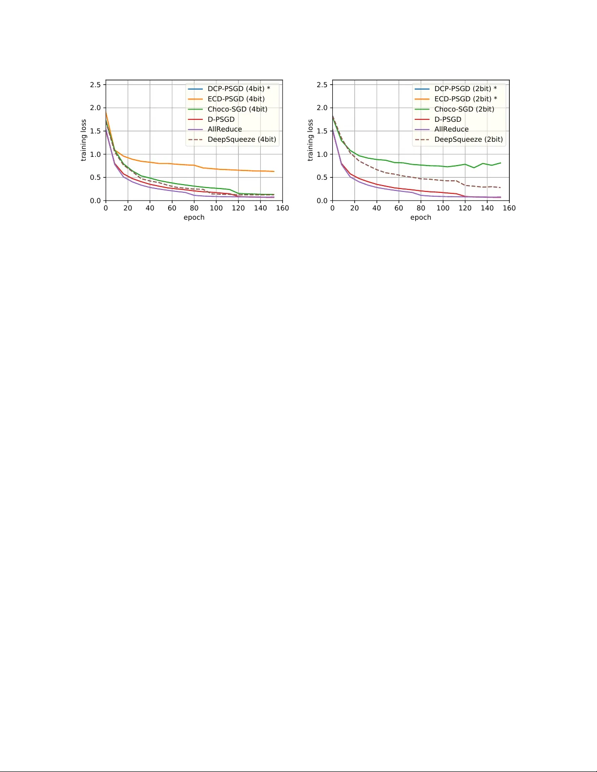
DeepSqueeze : Decen tralization Meets Error-Comp ensated Compression Hanlin T ang 1 , Xiangru Lian 1 , Sh uang Qiu 5 , Lei Y uan 3 , Ce Zhang 4 , T ong Zhang 2 , and Ji Liu 3,1 1 Departmen t of Computer Science, Universit y of Ro chester 2 Hong K ong Universit y of Science and T ec hnology 3 Seattle AI Lab, F eD A Lab, Kw ai Inc 4 Departmen t of Computer Science, ETH Zurich 5 Univ ersity of Mic higan August 6, 2019 Abstract Comm unication is a k ey b ottlenec k in distributed training. Recently , an err or-c omp ensate d compression tec hnology was particularly designed for the c entr alize d learning and receives h uge successes, by sho wing significan t adv an tages o ver state-of-the-art compression based methods in saving the comm unication cost. Since the de c entr alize d training has b een witnessed to be superior to the traditional centr alize d training in the communication restricted scenario, therefore a natural question to ask is “how to apply the error-comp ensated technology to the decentralized learning to further reduce the communication cost.” Ho wev er, a trivial extension of compression based centralized training algorithms do es not exist for the decen tralized scenario. key difference b et ween centralized and decentralized training makes this extension extremely non-trivial. In this pap er, we prop ose an elegan t algorithmic design to emplo y error-compensated sto c hastic gradient descen t for the decentralized scenario, named DeepSqueeze . Both the theoretical analysis and the empirical study are provided to sho w the prop osed DeepSqueeze algorithm outp erforms the existing compression based decentralized learning algorithms. T o the b est of our knowledge, this is the fi rst time to apply the error-comp ensated compression to the decentralized learning. 1 In tro duction W e consider the follo wing decen tralized optimization: min x ∈ R N f ( x ) = 1 n n X i =1 E ξ ∼D i F i ( x ; ξ ) | {z } =: f i ( x ) , (1) where n is the n umber of no de and D i is the local data distribution for no de i . n no des form a connected graph and eac h node can only comm unicate with its neigh b ors. Comm unication is a k ey bottleneck in distributed training [Abadi et al., 2016, Seide and Agarwal, 2016]. A p opular strategy to reduce communication cost is compressing the gradients computed on the lo cal w orkers and sending to the parameter serv er or a cen tral node. T o ensure the conv ergence, the compression usually needs to be unbiased and the compression ratio needs to b e c hosen very cautiously (it cannot b e to o aggressive), since the bias or noise caused b y the compression may significantly degrade the conv ergence efficiency . Recently , an error-comp ensated technology has been designed to make the aggressiv e compression 1 p ossible. The key idea is to store the compression error in the previous step and send the compressed sum of the gradient and the remaining compression error in the previous step [T ang et al., 2019]: g 0 ← C ω [ g + δ ] (compressed gradient on lo cal work er(s)) δ ← ( g + δ ) − C ω [ g + δ ] (remaining error on the lo cal work er(s)) x ← x − γ g 0 (up date on the parameter serv er) where g is the computed sto c hastic gradient. This idea has b een prov en to very effective and ma y significantly outp erform the traditional (non-error-comp ensated) compression centralized training algorithms such as Jiang and Agraw al [2018], Zhang et al. [2017]. The de c entr alize d training has b een pro v en to be superior to the c entr alize d training in terms of reducing the communication cost [Bo yd et al., 2006], especially when the model is huge and the net work bandwidth and latency are less satisfactory . The key reason is that in the decen tralized learning framework w ork ers only need to communicate with their individual neigh b ors, while in the cen tralized learning all w ork ers are required to talk to the cen tral node (or the parameter server). Moreo ver, the iteration complexit y (or the total computational complexity) of the decentralized learning is pro ven to b e comparable to that of the cen tralized coun terpart [Lian et al., 2017]. Therefore, giv en the recen t successes of the error-compensated tec hnology for the cen tralized learning, it motiv ates us to ask a natural question: How to apply the err or-c omp ensate d te chnolo gy to the de c entr alize d le arning to further r e duc e the c ommunic ation c ost? Ho wev er, k ey differences exist b et ween centralized and decentralized training, and it is highly non- trivial to extend the error-compensated tec hnology to decentralized learning. In this pap er, we prop ose an error-comp ensated decen tralized stochastic gradient metho d named DeepSqueeze b y com bining these t wo strategies. Both theoretical analysis and empirical study are pro vided to show the adv an tage of the prop osed DeepSqueeze algorithm ov er the existing compression based decentralized learning algorithms, including K olosko v a et al. [2019], T ang et al. [2018]. Our Con tribution: • T o the b est of our knowledge, this is the first time to apply the error-comp ensated compression tec hnology to decentralized learning. • Our algorithm is compatible with almost all compression strategies, and admits a muc h higher tolerance on aggressive compression ratio than existing work (for example, [T ang et al., 2018]) in b oth theory and empirical study . Notations and definitions Throughout this pap er, we use the following notations: • ∇ f ( · ) denotes the gradient of a function f . • f ∗ denotes the optimal v alue of the minimization problem (1). • f i ( x ) := E ξ ∼D i F i ( x ; ξ ) . • λ i ( · ) denotes the i -th largest eigen v alue of a symmetric matrix. • 1 = [1 , 1 , · · · , 1] > ∈ R n denotes the full-one v ector. • A n = 11 > n ∈ R n × n is an all 1 n square matrix. • k · k denotes the ` 2 norm for v ectors and the spectral norm for matrices. • k · k F denotes the v ector F rob enius norm of matrices. • C ω ( · ) denotes the compressing op erator. 2 The rest of the pap er is organized as follo ws. First w e review the related studies. W e then discuss our prop osed metho d in detail and pro vides k ey theoretical results. W e further v alidate our metho d in an exp erimen t and finally w e conclude this pap er. 2 Related W ork In this section, we review the recent works in a few areas that are closely related to the topic of this study: distributed learning, decentralized learning, compression based learning, and error-comp ensated compression metho ds. 2.1 Cen tralized P arallel Learning Distributed learning is an widely-used acceleration strategy for training deep neural netw ork with high computational cost. T w o main designs are dev elop ed to parallelize the computation: 1) cen tralized parallel learning [Agarw al and Duchi, 2011, Rech t et al., 2011], where all the work ers are ensured to obtain information from all others; 2) decentralized parallel learning [Dvurechenskii et al., 2018, He et al., 2018, Li and Y an, 2017, Lian et al., 2017], where eac h w orker can only gather information from a fraction of its neighbors. Centralized parallel learning requires a supporting net work architecture to aggregate all local models or gradien ts in each iteration. V arious implementations are dev elop ed for information aggregation in cen tralized systems. F or example, the parameter serv er [Abadi et al., 2016, Li et al., 2014], AllReduce [Renggli et al., 2018, Seide and Agarw al, 2016], adaptiv e distributed learning, differentially priv ate distributed learning, distributed pro ximal primal-dual algorithm, non-smo oth distributed optimization, pro jection-free distributed online learning, and parallel back-propagation for deep learning. 2.2 Decen tralized P arallel Learning Unlik e cen tralized learning, decentralized learning do es not require obtaining information from all w orkers in eac h step. Therefore, the netw ork structure w ould ha ve fewer restrictions than cen tralized parallel learning. Due to this high flexibilit y of the netw ork design, the decentralized parallel learning has b een the focus of man y recen t studies. In decentralized parallel learning, work ers only comm unicate with their neigh b ors. There are tw o main t yp es of decen tralized learning algorithms: fixed net w ork topology [He et al., 2018], or time-v arying [Lian et al., 2018, Nedić and Olshevsky, 2015] during training. Shen et al. [2018], W u et al. [2017] sho ws that the decen tralized SGD w ould con v erge with a comparable con vergence rate to the centralized algorithm with less needed communication to mak e large-scale mo del training feasible. Li et al. [2018] provide a systematic analysis of the decen tralized learning pip eline. 2.3 Compressed Comm unication Distributed Learning T o further reduce the comm unication o verhead, one promising direction is to compress the v ariables that are sent b et ween different work ers [Chen et al., 2018, W ang et al., 2018]. Previous w orks mostly focus on a cen tralized scenario where the compression is assumed to b e unbiased [Jiang and Agraw al, 2018, Shen et al., 2018, W angni et al., 2018, W en et al., 2017, Zhang et al., 2017]. A general theoretical analysis of centralized compressed parallel SGD can b e found in Alistarh et al. [2017]. Bey ond this, some biased compressing metho ds are also proposed and prov en to be quite efficient in reducing the comm unication cost. One example is the 1-Bit SGD [Seide et al., 2014], which compresses the en tries in gradien t v ector in to ± 1 depends on its sign. The theoretical guaran tee of this metho d is given in Bernstein et al. [2018]. Recen tly , another emerging area of compressed distributed learning is decen tralized compressed learning. Unlik e cen tralized setting, decentralized learning requires eac h w orker to share the mo del parameters, instead of the gradients. This differen tiating factor could p oten tial in v alidate the con vergence (see T ang et al. [2018] for example). Man y methods are proposed to solv e this problem. One idea is to use the difference of the 3 Algorithm 1 DeepSqueeze 1: Initialize : x 0 , learning rate γ , av eraging rate η , initial error δ = 0 , num b er of total iterations T , and w eight matrix W . 2: for t = 0 , . . . , T − 1 do 3: (On i -th no de) 4: Randomly sample ξ ( i ) t and compute lo cal sto c hastic gradien t g ( i ) t := ∇ F i ( x ( i ) t , ξ ( i ) t ) . 5: Compute the error-comp ensated v ariable up date v ( i ) t = x ( i ) t − γ g ( i ) t + δ ( i ) t . 6: Compr ess v ( i ) t in to C ω [ v ( i ) t ] and up date the error δ ( i ) t = v ( i ) t − C ω [ v ( i ) t ] . 7: Send compressed v ariable C ω [ v ( i ) t ] to the immediate neighbors of i -th node. 8: R e c eive C ω [ v ( j ) t ] from all neigh bors of i -th no de where j ∈ N ( i ) (notice that i ∈ N ( i ) ). 9: Up date lo cal mo del x ( i ) t +1 = x ( i ) t − γ g ( i ) t + η P j ∈N ( i ) ( W ij − I ij ) C ω [ v ( j ) t ] . 10: end for 11: Output : x . mo del updates as the shared information [T ang et al., 2018]. Kolosk o v a et al. [2019] further reduces the comm unication error b y sharing the difference of the mo del difference, but their result only considers a strongly con v ex loss function, which is not the case for no wada ys deep neural net work. T ang et al. [2018] also propose a extrap olation like strategy to control the compressing level. None of these w orks emplo y the error-comp ensate strategy . 2.4 Error-Comp ensated SGD In terestingly , an error-compensate strategy for AllReduce 1Bit-SGD is proposed in Seide et al. [2014], whic h can compensate the error in each iteration with quite less accuracy drop than training without the error- comp ensation. The error-comp ensation strategy is prov ed to b e able to potentially improv e the training efficiency for strongly conv ex loss function [Stich et al., 2018]. W u et al. [2018] further study an Error- Comp ensated SGD for quadratic optimization via adding t wo hyperparameters to comp ensate the error, but fail to theoretically verify the adv an tage of using error comp ensation. Most recently , T ang et al. [2019] give an theoretical analysis showing that in centralized learning, the error-compensation strategy is compatible with an arbitrary compression tec hnique and fundamentally proving why error-comp ensation admit an impro v ed con vergence rate with linear sp eedup for general non-con v ex loss function. Even though, their w ork only study the centralized distributed training. Whether error-compensation strategy can work b oth theoretically and empirically for decen tralized learning remains to b e inv estigated. W e will try to answ er these questions in this pap er. 3 Algorithm W e in tro duce our proposed DeepSqueeze algorithm details b elow. Consider that there are n w orkers in the netw ork, where each individual w orker (e.g., the i -th w ork er) can only comm unicate with its immediate neighbors (denotes work er i ’s immediate neigh b ors N ( i ) ). The connection can b e represented by a symmetric double sto c hastic matrix, the w eighted matrix W . W e denote b y W ij the weigh t betw een the i -th and j -th w orker. F or the i -th work er at time t , each w orker, sa y w orker i , need to maintain three main v ariables: the lo cal mo del x ( i ) t , the compression error δ ( i ) t , and the error-comp ensated v ariable v ( t ) t . The up dates of those v ariables follow the follo wing steps: 1. Lo cal Computation: Up date the error-compensated v ariable by v ( i ) t = x ( i ) t − γ ∇ F i ( x ( i ) t , ξ ( i ) t ) + δ ( i ) t where ∇ F i ( x ( i ) t , ξ ( i ) t ) is the stochastic gradient with randomly sampled ξ ( i ) t , and γ is the learning. 4 2. Lo cal Compression: Compress the error-comp ensated v ariable v ( i ) t in to C ω [ v ( i ) t ] , where C ω [ · ] is the compression op eration and up date the compression error b y δ ( i ) t = v ( i ) t − C ω [ v ( i ) t ] . 3. Global Comm unication: Send compressed v ariable C ω [ v ( i ) t ] to the neighbors of i -th no de, namely N ( i ) . 4. Lo cal Up date: Up date lo cal mo del by x ( i ) t +1 = x ( i ) t − γ g ( i ) t + η P j ∈N ( i ) ( W ij − I ij ) C ω [ v ( j ) t ] , where I denotes the iden tity matrix, and η is the a veraging rate. Finally , the prop osed DeepSqueeze algorithm is summarized in Algorithm 1. 4 Theoretical Analysis In this section, we introduce our theoretical analysis of DeepSqueeze . W e first prov e the updating rule of our algorithm to give an in tuitive explanation of ho w our algorithm w orks, then we present the final con vergence rate. 4.1 Mathematical form ulation In order to get a global view of DeepSqueeze , w e define X t := h x (1) t , x (2) t , · · · , x ( n ) t i ∈ R N × n , G ( X t ; ξ t ) := h ∇ F 1 ( x (1) t ; ξ (1) t ) , · · · , ∇ F n ( x ( n ) t ; ξ ( n ) t ) i , ∆ t := h δ (1) t , δ (2) t , · · · , δ ( n ) t i ∈ R N × n , ∇ f ( X t ) := E ξ G ( X t ; ξ t ) 1 n = 1 n n X i =1 ∇ f i  x ( i ) t  , x t := 1 n n X i =1 x ( i ) t . Then the up dating rule of DeepSqueeze follo ws X t +1 = X t − γ G t + η C ω [ X t − γ G t + ∆ t − 1 ] ( W − I ) ∆ t = X t − γ G t + ∆ t − 1 − C ω [ X t − γ G t + ∆ t − 1 ] , whic h can also be rewritten as X t +1 = ( X t − γ G t ) W eff + (∆ t − 1 − ∆ t )( W eff − I ) , where we denote W eff = (1 − η ) I + η W . 4.2 Wh y DeepSqueeze is b etter W e would b e able to get a b etter understanding ab out why DeepSqueeze is b etter than the other compression based decentralized algorithms, b y analyzing the clos ed forms of up dating rules. F or simplicity , we assume the initial v alues are 0 . Skipping the detailed deriv ation, we can obtain the closed forms: • D-PSGD [Lian et al., 2017] (without compression): X t = − γ t − 1 X s =0 G s W t − s eff . • DCD-PSGD [T ang et al., 2018] (with compression): X t = − γ t − 1 X s =0 G s W t − s eff − η t − 2 X s =0 ∆ s W t − s eff . 5 • CHCHO-SGD [Kolosk ov a et al., 2019] (with compression): X t = − γ t − 1 X s =0 G s W t − s eff − η t − 1 X s =0 ∆ s ( W eff − I ) W t − s eff . • Updating rule of DeepSqueeze (with error-comp ensated compression): X t = − γ t − 1 X s =0 G s W t − s eff − η ∆ t − 1 ( W eff − I ) + η t − 2 X s =0 ∆ s ( W eff − I ) 2 W t − s eff . W e can notice that if ∆ s = 0 , that is, there is no compression error, all compression based metho ds reduce to D-PSGD. Therefore the efficiency of compression based metho ds lie on the magnitude of k ∆ s k F (for D-PSGD) or k ∆ s ( W eff ) − I k F (for DeepSqueeze and CHCHO-SGD). Using the fact that W is doubly sto c hastic and symmetric, w e hav e k W eff − I k 2 = k η W − η I k ≤ η (1 − λ n ( W )) , whic h leads to   ∆ s ( W eff − I ) 2   2 F ≤   ( W eff − I ) 2   2 k ∆ s k 2 F ≤ (1 − λ n ( W )) 4 η 4 k ∆ s k 2 F ( DeepSqueeze ) k ∆ s ( W eff − I ) k 2 F ≤k W eff − I k 2 k ∆ s k 2 F ≤ (1 − λ n ( W )) 2 η 2 k ∆ s k 2 F (CHOCO-SGD) k ∆ s k 2 F ≤ k ∆ s k 2 F . (DCD-PSGD) whic h means our algorithm could be able to significan tly reducing the influence of the history compressing error b y controlling η . Actually , it will b e clear so on (from our analysis), η has to b e small enough if w e compress the information v ery aggressive. Before we introducing the final con vergence rate of DeepSqueeze , we first in troduce some assumptions that is used for theoretical analysis. Assumption 1. Thr oughout this p ap er, we make the fol lowing c ommonly use d assumptions: 1. Lipschitzian gr adient: Al l function f i ( · ) ’s ar e with L -Lipschitzian gr adients. 2. Symmetric double sto chastic matrix: The weighte d matrix W is a r e al double sto chastic matrix that satisfies W = W > and W 1 = W . 3. Sp e ctr al gap: Given the symmetric doubly sto chastic matrix W , we assume that λ 2 ( W ) ≤ 1 . 4. Start fr om 0: W e assume X 0 = 0 . This assumption simplifies the pr o of w.l.o.g. 5. Bounde d varianc e: Assume the varianc e of sto chastic gr adient to b e b ounde d E ξ ∼D i k∇ F i ( x ; ξ ) − ∇ f i ( x ) k 2 6 σ 2 , Inner varianc e 1 n n X i =1 k∇ f i ( x ) − ∇ f ( x ) k 2 6 ζ 2 , ∀ i, ∀ x , Outer varianc e 6. Bounde d Signal-to-noise factor: The magnitude of the c ompr ession err or is assume d to b e b ounde d by the original ve ctor’s magnitude: E k C ω [ x ] − x k 2 ≤ α 2 k x k 2 , α ∈ [0 , 1) , ∀ x . 6 Notice that these assumptions are quite standard for analyzing decentralized algorithms in previous w orks Lian et al. [2017]. Unlike K olosko v a et al. [2019], we do not require the gradien t to b e b ounded ( k∇ f ( x ) k ≤ G 2 ), whic h makes our result more applicable to a general case. It is worth p ointing out that man y of the previous compressing strategies satisfy the b ounded signal-to-noise factor assumption, suc h as GSpar, random sparsification [W angni et al., 2018], top- k sparsification and random quan tization [K olosko v a et al., 2019]. No w w e are ready to show the main theorem of DeepSqueeze . Theorem 1. F or DeepSqueeze , if the aver aging r ate η and le arning r ate γ satisfies η ≤ min ( 1 2 , α − 2 3 − 1 4 ) 1 − 3 C 2 L 2 γ 2 ≥ 0 γ ≤ 1 L , then we have  γ 2 − 3 C 3 γ 3  T X t =0 E k∇ f ( x t ) k 2 ≤ E f ( x 0 ) − E f ( x T ) +  Lγ 2 2 n + C 3 γ 3  σ 2 T + 3 C 3 γ 3 ζ 2 , wher e C 0 := η (1 − λ n ( W )) C 1 := α 2  1 − α 2 (1 + C 0 ) 2 (1 + 2 C 0 )  C 2 0 C 2 := 3 η 2 (1 − λ 2 ( W )) 2 + 6 C 1 C 3 := C 2 L 2 2 − 6 C 2 L 2 γ 2 . T o mak e the result more clear, w e c ho ose the learning rate γ appropriately in the follo wing: Corollary 1. A c c or ding to The or em 1, cho osing γ = 1 3 L √ C 2 + σ √ T n + ζ 2 3 T 1 3 and η = min  1 2 , α − 2 3 − 1 4  , we have the fol lowing c onver genc e r ate for DeepSqueeze 1 T T X t =0 E k∇ f ( x t ) k 2 .  1 √ nT + C 2 T  σ + C 2 ζ 2 3 T 2 3 + 1 T , wher e we have C 2 . 1 (1 − λ 2 ( W )) 2   1 + α 2  α − 2 3 − 1    . wher e L is tr e ate d to b e a c onstant. This result suggests that: 7 Linear sp eedup The asymptotical con vergence rate of DeepSqueeze is O  1 / √ nT  , which is exactly the same with Cen tralized P arallel SGD. Consistence with D-PSGD Setting α = 0 , our DeepSqueeze reduces to the standard decentralized SGD (D-PSGD), our result indicates that the con vergence rate admits O  σ √ nT + ζ 2 3 T 2 3  , which is sligh tly b etter than the previous one O  σ √ nT + n 2 3 ζ 2 3 T 2 3  in Lian et al. [2017]. Sup eriorit y o ver DCD-PSD and ECD-PSGD By using the error-comp ensate strategy , we prov e that the the dep endence to the compression ratio α is O  σ α 2 T + ζ 2 3 α 2 T 2 3  , and is robust to any compression op erator with α ∈ [0 , 1) . Whereas the previous work [T ang et al., 2018] only ensure a dep endence O  σ α 2 √ T + ζ 2 3 α 2 T 2 3  and there is a restriction that α ≤ (1 − λ 2 ( W )) 2 . Balance b et ween Communication and Computation: Our result indicates that when α → 1 , w e need to set η to be small enough to ensure the con vergence of our algorithm. How ever, too small η leads to a slo wer conv ergence rate, which means more iterations are needed for training. Our result could be a guidance for balancing the comm unication cost and computation cost for decen tralized learning under differen t situations. 5 Exp erimen ts In this section, we further demonstrate the superiority of the DeepSqueeze algorithm through an empirical study . Under aggressiv e compression ratios, we show the ep och-wise con vergence results of DeepSqueeze and compare them with centralized SGD (AllReduce), decentralized SGD without compression (D-PSGD [Lian et al., 2017]), and other existing decen tralized compression algorithms (ECP-PSGD, DCP-PSGD [T ang et al., 2018], and Cho co-SGD [Kolosk o v a et al., 2019]). 5.1 Exp erimen tal Setup Dataset W e b enchmark the algorithms with a standard image classification task: CIF AR10 using ResNet-20. This dateset has a training set of 50,000 images and a test set of 10,000 images, where each image is given one of the 10 lab els. Comm unication The communication is implemented based on NVIDIA NCCL for AllReduce and gloo for all other algorithms. The work ers are connected in a ring netw ork so that eac h w orker has t wo neighbors. Compression W e use bit compression for all the compression algorithms, where every element of the tensor sen t out or received by a w orker is compressed to 4 bits or 2 bits. A n um b er representing the Euclidean norm of the original tensor is also sen t together, so that when a work er receiv es the compressed tensor, it can scale it to get a tensor with the same Euclidean norm as the uncompressed tensor. Hardw are The experiments are done on 8 2080Ti GPUs, where eac h GPU is treated as a single w orker in the algorithm. 5.2 Con v ergence Efficiency W e compare the algorithms with 4bit and 2bit compression, and the conv ergence results are shown in Figure 1. W e use a batch size of 128 and tune the learning rate in a { 1 , 0 . 5 , 0 . 1 , 0 . 01 } set for eac h algorithm. The learning rate is decreased by 5x ev ery 60 ep o c hs. 8 0 20 40 60 80 100 120 140 160 epoch 0.0 0.5 1.0 1.5 2.0 2.5 training loss DCP-PSGD (4bit) * ECD-PSGD (4bit) Choco-SGD (4bit) D-PSGD AllReduce DeepSqueeze (4bit) 0 20 40 60 80 100 120 140 160 epoch 0.0 0.5 1.0 1.5 2.0 2.5 training loss DCP-PSGD (2bit) * ECD-PSGD (2bit) * Choco-SGD (2bit) D-PSGD AllReduce DeepSqueeze (2bit) Figure 1: Epo ch-wise conv ergence for the algorithms with 8 work ers connected on a ring netw ork. 4bit compression is on the left and 2bit compression is on the righ t. Note that DCP-PSGD (marked with *) do es not con v erge b elo w 4bit compression as stated in the original paper [T ang et al., 2018], and ECP-PSGD does not conv erge under 2bit compression, so they are not shown in the figure. Note that, compared with uncompressed metho ds, 4bit compression sav es 7/8 of the communication cost while 2bit compress ion reduces the cost b y 93.75%. The results show that under 4bit compression, DeepSqueeze con verges similar to uncompressed algorithms. DeepSqueeze is sligh tly b etter than Cho co-SGD [K olosko v a et al., 2019], and conv erges m uc h faster than DCP-PSGD and ECD-PSGD. Note that DCP-PSGD do es not conv erge under 4bit compression (as stated in the original pap er [T ang et al., 2018]), and ECD-PSGD do es not conv erge under 2bit compression. Under 2bit compression, DeepSqueeze con verges slow er than uncompressed algorithms, but is still faster than any other compression algorithms. The reason is that the less bits we hav e, the more we gain from the error compensation in DeepSqueeze , and consequen tly DeepSqueeze gets a faster con vergence. The experimental results further confirm that DeepSqueeze ac hieves outstanding comm unication cost reduction (up to 93.75%) without m uch sacrifice on conv ergence. 6 Conclusion This pap er applies the error-compensated compression strategy , whic h receiv es big successes in cen tralized training, to the decen tralized training. Through elab orated algorithm, the prop osed DeepSqueeze algorithms is pro ven to admit higher tolerance on the compression ratio than existing compression based decen tralized training. Both theoretical analysis and empirical study v alidate our algorithm and theorem. 9 References M. Abadi, P . Barham, J. Chen, Z. Chen, A. Da vis, J. Dean, M. Devin, S. Ghema wat, G. Irving, M. Isard, M. Kudlur, J. Leven b erg, R. Monga, S. Mo ore, D. G. Murray , B. Steiner, P . T uck er, V. V asudev an, P . W arden, M. Wick e, Y. Y u, and X. Zheng. T ensorflow: A system for large-scale mac hine learning. In Pr o c e e dings of the 12th USENIX Confer enc e on Op er ating Systems Design and Implementation , OSDI’16, pages 265–283, Berk eley , CA, USA, 2016. USENIX Association. ISBN 978-1-931971-33-1. A. Agarwal and J. C. Duchi. Distributed dela yed sto c hastic optimization. In A dvanc es in Neur al Information Pr o c essing Systems , pages 873–881, 2011. D. Alistarh, D. Grubic, J. Li, R. T omiok a, and M. V o jno vic. QSGD: comm unication-efficient SGD via gradien t quan tization and enco ding. In I. Guyon, U. v on Luxburg, S. Bengio, H. M. W allach, R. F ergus, S. V. N. Vish wanathan, and R. Garnett, editors, A dvanc es in Neur al Information Pr o c essing Systems 30: Annual Confer enc e on Neur al Information Pr o c essing Systems 2017, 4-9 De c emb er 2017, L ong Be ach, CA, USA , pages 1707–1718, 2017. J. Bernstein, J. Zhao, K. Azizzadenesheli, and A. Anandkumar. signsgd with ma jority vote is comm unication efficien t and byzan tine fault tolerant. 10 2018. S. Bo yd, A. Ghosh, B. Prabhak ar, and D. Shah. Randomized gossip algorithms. IEEE tr ansactions on information the ory , 52(6):2508–2530, 2006. T. Chen, G. Giannakis, T. Sun, and W. Yin. Lag: Lazily aggregated gradien t for communication-efficien t distributed learning. In S. Bengio, H. W allach, H. Laro c helle, K. Grauman, N. Cesa-Bianchi, and R. Garnett, editors, A dvanc es in Neur al Information Pr o c essing Systems 31 , pages 5055–5065. Curran Asso ciates, Inc., 2018. P . Dvurec henskii, D. Dvinskikh, A. Gasnik ov, C. Urib e, and A. Nedich. Decen tralize and randomize: F aster algorithm for w asserstein barycenters. In S. Bengio, H. W allach, H. Laro c helle, K. Grau- man, N. Cesa-Bianchi, and R. Garnett, editors, A dvanc es in Neur al Information Pr o c essing Sys- tems 31 , pages 10760–10770. Curran Asso ciates, Inc., 2018. URL http://papers.nips.cc/paper/ 8274- decentralize- and- randomize- faster- algorithm- for- wasserstein- barycenters.pdf . L. He, A. Bian, and M. Jaggi. Cola: Decentralized linear learning. In A dvanc es in Neur al Information Pr o c essing Systems , pages 4541–4551, 2018. P . Jiang and G. Agraw al. A linear sp eedup analysis of distributed deep learning with sparse and quan tized comm unication. In S. Bengio, H. W allach, H. Larochelle, K. Grauman, N. Cesa-Bianc hi, and R. Garnett, editors, A dvanc es in Neur al Information Pr o c essing Systems 31 , pages 2530–2541. Curran Asso ciates, Inc., 2018. A. Kolosk ov a, S. U. Stich, and M. Jaggi. Decentralized sto chastic optimization and gossip algorithms with compressed com m unication. CoRR , abs/1902.00340, 2019. URL . M. Li, D. G. Andersen, J. W. Park, A. J. Smola, A. Ahmed, V. Josifo vski, J. Long, E. J. Shekita, and B.-Y. Su. Scaling distributed mac hine learning with the parameter server. In OSDI , volume 14, pages 583–598, 2014. Y. Li, M. Y u, S. Li, S. A v estimehr, N. S. Kim, and A. Sch wing. Pip e-sgd: A decen tralized pip elined sgd framew ork for distributed deep net training. In S. Bengio, H. W allac h, H. Laro c helle, K. Grauman, N. Cesa-Bianchi, and R. Garnett, editors, A dvanc es in Neur al Information Pr o c essing Systems 31 , pages 8056–8067. Curran Asso ciates, Inc., 2018. Z. Li and M. Y an. A primal-dual algorithm with optimal stepsizes and its application in decentralized consensus optim ization. arXiv pr eprint arXiv:1711.06785 , 2017. 10 X. Lian, C. Zhang, H. Zhang, C.-J. Hsieh, W. Zhang, and J. Liu. Can dec en tralized algorithms outperform cen tralized algorithms? a case study for decentralized parallel sto c hastic gradien t descen t. In A dvanc es in Neur al Information Pr o c essing Systems , pages 5330–5340, 2017. X. Lian, W. Zhang, C. Zhang, and J. Liu. Async hronous decen tralized parallel sto c hastic gradient descent. In International Confer enc e on Machine L e arning , 2018. A. Nedić and A. Olshevsky . Distributed optimization o ver time-v arying directed graphs. IEEE T r ansactions on Automatic Contr ol , 60(3):601–615, 2015. B. Rech t, C. Re, S. W right, and F. Niu. Hogwild: A lo c k-free approac h to parallelizing stochastic gradient descen t. In A dvanc es in neur al information pr o c essing systems , pages 693–701, 2011. C. Renggli, D. Alistarh, and T. Ho efler. Sparcml: High-p erformance sparse comm unication for machine learning. arXiv pr eprint arXiv:1802.08021 , 2018. F. Seide and A. Agarw al. Cntk: Microsoft’s op en-source deep-learning toolkit. In Pr o c e e dings of the 22nd ACM SIGKDD International Confer enc e on Know le dge Disc overy and Data Mining , pages 2135–2135. A CM, 2016. F. Seide, H. F u, J. Dropp o, G. Li, and D. Y u. 1-bit sto c hastic gradient descen t and application to data-parallel distributed training of speech dnns. In Intersp e e ch 2014 , Septem b er 2014. Z. Shen, A. Mokhtari, T. Zhou, P . Zhao, and H. Qian. T ow ards more efficient sto c hastic decentralized learning: F aster con vergence and sparse communication. In J. Dy and A. Krause, editors, Pr o c e e dings of the 35th International Confer enc e on Machine L e arning , v olume 80 of Pr o c e e dings of Machine L e arning R ese ar ch , pages 4624–4633, Sto c kholmsmässan, Stockholm Sweden, 10–15 Jul 2018. PMLR. S. U. Stich, J.-B. Cordonnier, and M. Jaggi. Sparsified sgd with memory . In S. Bengio, H. W allach, H. Laro c helle, K. Grauman, N. Cesa-Bianchi, and R. Garnett, editors, A dvanc es in Neur al Information Pr o c essing Systems 31 , pages 4452–4463. Curran Asso ciates, Inc., 2018. H. T ang, S. Gan, C. Zhang, T. Zhang, and J. Liu. Communication compression for decentralized training. In S. Bengio, H. W allac h, H. Larochelle, K. Grauman, N. Cesa-Bianc hi, and R. Garnett, editors, A dvanc es in Neur al Information Pr o c essing Systems 31 , pages 7663–7673. Curran Asso ciates, Inc., 2018. H. T ang, X. Lian, T. Zhang, and J. Liu. Doublesqueeze: P arallel stochastic gradient descent with double-pass error-comp ensated compression. In Thirty-sixth International Confer enc e on Machine L e arning , 2019. H. W ang, S. Siev ert, S. Liu, Z. Charles, D. P apailiop oulos, and S. W righ t. Atomo: Communication-efficien t learning via atomic sparsification. In S. Bengio, H. W allac h, H. Laro chelle, K. Grauman, N. Cesa-Bianc hi, and R. Garnett, editors, A dvanc es in Neur al Information Pr o c essing Systems 31 , pages 9872–9883. Curran Asso ciates, Inc., 2018. J. W angni, J. W ang, J. Liu, and T. Zhang. Gradien t sparsification for comm unication-efficien t distributed optimization. In S. Bengio, H. W allac h, H. Laro c helle, K. Grauman, N. Cesa-Bianc hi, and R. Garnett, editors, A dvanc es in Neur al Information Pr o c essing Systems 31 , pages 1306–1316. Curran Asso ciates, Inc., 2018. W. W en, C. Xu, F. Y an, C. W u, Y. W ang, Y. Chen, and H. Li. T erngrad: T ernary gradien ts to reduce comm unication in distributed deep learning. In I. Guyon, U. V. Luxburg, S. Bengio, H. W allac h, R. F ergus, S. Vish wanathan, and R. Garnett, editors, A dvanc es in Neur al Information Pr o c essing Systems 30 , pages 1509–1519. Curran Asso ciates, Inc., 2017. J. W u, W. Huang, J. Huang, and T. Zhang. Error comp ensated quantized SGD and its applications to large-scale distributed optimization. In J. Dy and A. Krause, editors, Pr o c e e dings of the 35th International Confer enc e on Machine L e arning , volume 80 of Pr o c e e dings of Machine L e arning R ese ar ch , pages 5325–5333, Sto c kholmsmässan, Sto ckholm Sweden, 10–15 Jul 2018. PMLR. 11 T. W u, K. Y uan, Q. Ling, W. Yin, and A. H. Say ed. Decentralized consensus optimization with async hron y and delays. IEEE T r ansactions on Signal and Information Pr o c essing over Networks , PP:1–1, 04 2017. doi: 10.1109/TSIPN.2017.2695121. H. Zhang, J. Li, K. Kara, D. Alistarh, J. Liu, and C. Zhang. ZipML: T raining linear models with end-to-end lo w precision, and a little bit of deep learning. In D. Precup and Y. W. T eh, editors, Pr o c e e dings of the 34th International Confer enc e on Machine L e arning , v olume 70 of Pr o c e e dings of Machine L e arning R ese ar ch , pages 4035–4043, In ternational Con ven tion Cen tre, Sydney , Australia, 06–11 Aug 2017. PMLR. 12 Supplemen tary Material W e pro vide the pro ofs to our theorems in the supplemen tal material. Preliminaries Belo w w e w ould use some basic prop erties of matrix and v ector. • F or an y A ∈ R d × n and P ∈ R n × n , if P P > = I , then we ha ve k AP k 2 F = k AP > k 2 F = k A k 2 F . • F or an y t wo vectors a and b , w e ha ve k a + b k 2 ≤ (1 + α ) k a k 2 +  1 + 1 α  k b k 2 , ∀ α > 0 . • F or an y t wo matrices A and B , w e hav e k A + B k 2 F ≤ (1 + α ) k A k 2 F +  1 + 1 α  k B k 2 F , ∀ α > 0 . Before presenting our pro of, we first rewrite our updating rule as follo ws ∆ t =( X t − γ G t ) + ∆ t − 1 − C ω [( X t − γ G t ) + ∆ t − 1 ] X t +1 =( X t − γ G t ) W eff + η (∆ t − 1 − ∆ t )( W eff − I ) (2) where W eff := (1 − η ) I + η W. Pro of of Lemma 1 Lemma 1 is the key lemma for pro ving our Theorem 1. Lemma 1. F or algorithm that admits the up dating rule (2) , if W eff  0 , (2 − λ n ) 2 (3 − 2 λ n ) ≤ 1 α 2 , 1 − 3 C 5 L 2 γ 2 ≥ 0 , L ≤ 1 L then we have  γ 2 − 3 C 5 L 2 γ 3 2 − 6 C 5 L 2 γ 2  T X t =0 E k∇ f ( x t ) k 2 ≤ E f ( x 0 ) − E f ( x ∗ ) +  Lγ 2 2 + C 5 L 2 γ 3 2 − 6 C 5 L 2 γ 2 )  σ 2 T + 3 C 5 L 2 γ 3 ζ 2 T 2 − 6 C 5 L 2 γ 2 . 13 wher e C 4 := α 2 (1 − α 2 (2 − λ n ) 2 (3 − 2 λ n ))(1 − λ n ) 2 C 5 := 3 (1 − λ 2 ) 2 + 6 C 4 , and λ n = λ n ( W eff ) and λ 2 = λ 2 ( W eff ) for short. W e outline our proof of Lemma 1 as follo ws. The most challenging part of a decen tralized algorithm, unlik e the cen tralized algorithm, is that we need to ensure the local model on each no de to con verge to the av erage v alue x t . This is because E f ( x t +1 ) − E f ( x t ) ≤ − γ 2 E   ∇ f ( X t )   2 −  γ 2 − Lγ 2 2  E   ∇ f ( X t )   2 + γ L 2 2 n E k X t ( I − A n ) k 2 F + Lγ 2 σ 2 2 n . (3) So we first pro ve that T − 1 X t =0 n X i =1    x t − x ( i ) t    2 = T − 1 X t =0 E k X t ( I − A n ) k 2 F ≤ 3 γ 2 (1 − λ 2 ) 2 T − 2 X t =0 k G t k 2 F + 6 T − 1 X t =0 k ∆ t ( W eff − I ) k 2 F , and the compressing error can be upper bounded b y T − 1 X t =0 E k ∆ t ( W eff − I ) k 2 ≤ C 4 γ 2 T − 1 X t =0 E k G t k 2 F . With these t wo imp ortan t observ ations, w e finally prov e that T − 1 X t =0 E k X t ( I − A n ) k 2 F ≤ C 5 γ 2 nσ 2 T 1 − 3 C 5 L 2 γ 2 + 3 nC 5 γ 2 ζ 2 T 1 − 3 C 5 L 2 γ 2 + T − 1 X t =0 3 nC 5 γ 2 E k∇ f ( x t ) k 2 1 − 3 C 5 L 2 γ 2 . So taking the equation ab o ve in to (3) we could directly prov e Theorem 1. No w w e in tro duce the detailed pro of for Lemma 1. Pro of of Lemma 1 Pr o of. The updating rule of DeepSqueeze can be written as ∆ t = − γ G t + X t + ∆ t − 1 − C ω [ − γ G t + X t + ∆ t − 1 ] , X t +1 =( X t − γ G t ) W eff + (∆ t − 1 − ∆ t )( W eff − I ) , The up dating rule of x t can b e conducted using the equation abov e x t +1 = x t − γ G t . So we hav e E f ( x t +1 ) − E f ( x t ) ≤ − γ E  G t , ∇ f ( x t )  + Lγ 2 2 E   G t   2 14 = − γ E  ∇ f ( X t ) , ∇ f ( x t )  + Lγ 2 2 E   G t − ∇ f ( X t )   2 + Lγ 2 2 E   ∇ f ( X t )   2 = − γ E  ∇ f ( X t ) , ∇ f ( x t )  + Lγ 2 2 E   ∇ f ( X t )   2 + Lγ 2 σ 2 2 n . Using  ∇ f ( X t ) , ∇ f ( x t )  = 1 2    ∇ f ( X t )   2 + k∇ f ( x t ) k 2 −   ∇ f ( X t ) − ∇ f ( x t )   2  , then the equation abov e b ecomes E f ( x t +1 ) − E f ( x t ) ≤ − γ 2  E   ∇ f ( X t )   2 + E k∇ f ( x t ) k 2 − E   ∇ f ( X t ) − ∇ f ( x t )   2  + Lγ 2 2 E   ∇ f ( X t )   2 + Lγ 2 σ 2 2 n = − γ 2 E k∇ f ( x t ) k 2 −  γ 2 − Lγ 2 2  E   ∇ f ( X t )   2 + γ 2 E   ∇ f ( X t ) − ∇ f ( x t )   2 + Lγ 2 σ 2 2 n . (4) The differenc e b et ween ∇ f ( X t ) and ∇ f ( x t ) can b e upp er b ounded b y E   ∇ f ( X t ) − ∇ f ( x t )   2 = E      1 n n X i =1 ∇ f i ( x ( i ) t ) − ∇ f i ( x t )      2 ≤ 1 n 2 E      n X i =1 ∇ f i ( x ( i ) t ) − ∇ f i ( x t )      2 ≤ 1 n n X i =1 E    ∇ f i ( x ( i ) t ) − ∇ f i ( x t )    2 ≤ L 2 n n X i =1 E    x ( i ) t − x t    2 = L 2 n E k X t ( I − A n ) k 2 F . So (4) b ecomes E f ( x t +1 ) − E f ( x t ) ≤ − γ 2 E k∇ f ( x t ) k 2 −  γ 2 − Lγ 2 2  E   ∇ f ( X t )   2 + γ L 2 2 n E k X t ( I − A n ) k 2 F + Lγ 2 σ 2 2 n . Con tinuing using Lemma 7 to give upp er b ound for E k X t ( I − A n ) k 2 F , we hav e E f ( x t +1 ) − E f ( x t ) ≤ − γ 2 E   ∇ f ( X t )   2 −  γ 2 − Lγ 2 2  E   ∇ f ( X t )   2 + γ L 2 2 n E k X t ( I − A n ) k 2 F + Lγ 2 σ 2 2 n ≤ − γ 2 E k∇ f ( x t ) k 2 −  γ 2 − Lγ 2 2  E   ∇ f ( X t )   2 + Lγ 2 σ 2 2 n + C 5 L 2 γ 3 σ 2 2 − 6 C 5 L 2 γ 2 ) + 3 C 5 L 2 γ 3 ζ 2 2 − 6 C 5 L 2 γ 2 + 3 C 5 L 2 γ 3 E k∇ f ( x t ) k 2 2 − 6 C 5 L 2 γ 2 , 15 whic h can b e rewritten as  γ 2 − 3 C 5 L 2 γ 3 2 − 6 C 5 L 2 γ 2  E k∇ f ( x t ) k 2 ≤ E f ( x t ) − E f ( x t +1 ) −  γ 2 − Lγ 2 2  E   ∇ f ( X t )   2 +  Lγ 2 2 n + C 5 L 2 γ 3 2 − 6 C 5 L 2 γ 2 )  σ 2 + 3 C 5 L 2 γ 3 ζ 2 2 − 6 C 5 L 2 γ 2 . Summing up the equation ab o ve from t = 0 to t = T − 1 we get  γ 2 − 3 C 5 L 2 γ 3 2 − 6 C 5 L 2 γ 2  T X t =0 E k∇ f ( x t ) k 2 ≤ E f ( x 0 ) − E f ( x T ) +  Lγ 2 2 n + C 5 L 2 γ 3 2 − 6 C 5 L 2 γ 2  σ 2 T + 3 C 5 L 2 γ 3 ζ 2 T 2 − 6 C 5 L 2 γ 2 . ( γ ≤ 1 L ) This conclud es the proof. Belo w are some critical lemmas for the pro of of Lemma 1. Lemma 2. Given two non-ne gative se quenc es { a t } ∞ t =1 and { b t } ∞ t =1 that satisfying a t = t X s =1 ρ t − s b s , (5) with ρ ∈ [0 , 1) , we have D k := k X t =1 a 2 t ≤ 1 (1 − ρ ) 2 k X s =1 b 2 s . Pr o of. F rom the definition, w e ha ve S k = k X t =1 t X s =1 ρ t − s b s = k X s =1 k X t = s ρ t − s b s = k X s =1 k − s X t =0 ρ t b s ≤ k X s =1 b s 1 − ρ , (6) D k = k X t =1 t X s =1 ρ t − s b s t X r =1 ρ t − r b r = k X t =1 t X s =1 t X r =1 ρ 2 t − s − r b s b r ≤ k X t =1 t X s =1 t X r =1 ρ 2 t − s − r b 2 s + b 2 r 2 = k X t =1 t X s =1 t X r =1 ρ 2 t − s − r b 2 s ≤ 1 1 − ρ k X t =1 t X s =1 ρ t − s b 2 s ≤ 1 (1 − ρ ) 2 k X s =1 b 2 s . (due to (6)) 16 Lemma 3. F or any matrix se quenc e { M t } and p ositive inte ger c onstant m ∈ { 1 , 2 , · · · } , we have T − 1 X t =0      t X s =0 M s ( W eff − I ) m W t − s eff      2 F ≤ (1 − λ n ) 2 m − 2 T − 1 X t =0 k M t k 2 F . Pr o of. Since W eff is symmetric, so we decomp ose it as W eff = P Λ P > . Denote B s := M s P > and b ( i ) s b e the i th column of B s , we hav e      t X s =0 M s ( W eff − I ) m W t − s eff      2 F =      t X s =0 M s P > (Λ − I ) m Λ t − s P      2 F =      t X s =0 M s P > (Λ − I ) m Λ t − s      2 F =      t X s =0 B s (Λ − I ) m Λ t − s      2 F = n X i =1      t X s =0 b ( i ) s ( λ i − 1) m λ t − s i      2 = n X i =1 ( λ i − 1) 2 m      t X s =0 b ( i ) s λ t − s i      2 . So we hav e T − 1 X t =0      t X s =0 M s ( W eff − I ) m W t − s eff      2 F = T − 1 X t =0 n X i =1 ( λ i − 1) 2 m      t X s =0 b ( i ) s λ t − s i      2 = n X i =1 ( λ i − 1) 2 m T − 1 X t =0      t X s =0 b ( i ) s λ t − s i      2 ≤ n X i =1 ( λ i − 1) 2 m 1 (1 − λ i ) 2 T − 1 X t =0    b ( i ) t    2 ! (using Lemma 2) = n X i =1 ( λ i − 1) 2 m (1 − λ i ) 2 T − 1 X t =0    b ( i ) t    2 ≤ (1 − λ n ) 2 m − 2 T − 1 X t =0 n X i =1    b ( i ) t    2 =(1 − λ n ) 2 m − 2 T − 1 X t =0 k M t k 2 F . Lemma 4. F or AlgXX, we have the fol lowing upp er b ound for E k ∆ t ( W eff − I ) k 2 F : T − 1 X t =0 E k ∆ t ( W eff − I ) k 2 ≤ C 4 γ 2 T − 1 X t =0 E k G t k 2 F , 17 when (2 − λ n ) 2 (3 − 2 λ n ) ≤ 1 α 2 . Pr o of. F rom Assumption XXX, for ∆ t , we hav e E k ∆ t ( W eff − I ) k 2 F ≤ E α 2 k ( X t − γ G t + ∆ t − 1 ) ( W eff − I ) k 2 F = α 2 E      − γ t X s =0 G s W t − s eff ( W eff − I ) + t − 2 X s =0 ∆ s ( W eff − I ) 3 W t − 2 − s eff − ∆ t − 1 ( W eff − I ) 2 + ∆ t − 1 ( W eff − I )      2 F ≤ α 2 E  1 + 1 β 1       − γ t X s =0 G s W t − s eff ( W eff − I ) + t − 2 X s =0 ∆ s ( W eff − I ) 3 W t − 2 − s eff      2 F + α 2 (1 + β 1 ) E k ∆ t − 1 (2 I − W eff )( W eff − I ) k 2 F ≤ α 2  1 + 1 β 1  (1 + β 2 ) E      t − 2 X s =0 ∆ s ( W eff − I ) 3 W t − 2 − s eff      2 F + α 2  1 + 1 β 1   1 + 1 β 2  E      − γ t X s =0 G s W t − s eff ( W eff − I )      2 F + α 2 (1 + β 1 )(2 − λ n ) 2 E k ∆ t − 1 ( W eff − I ) k 2 . (7) Defining ∆ − 1 = ∆ − 2 = 0 , and b ound    P t − 2 s =0 ∆ s ( W eff − I ) 3 W t − 2 − s eff    2 F in the equation abov e using Lemma 3, whic h leads to T − 1 X t =0      t − 2 X s = − 2 ∆ s ( W eff − I ) 3 W t − 2 − s eff      2 F = T − 3 X t = − 2      t X s = − 2 ∆ s ( W eff − I ) 3 W t − s eff      2 F = T − 3 X t =0      t X s =0 ∆ s ( W eff − I ) 3 W t − s eff      2 F ( ∆ − 1 = ∆ − 2 = 0 ) ≤ (1 − λ n ) 2 T − 3 X t =0 k ∆ t ( W eff − I ) k 2 F . (8) Setting β 1 = β 2 = 1 − λ n , summing up both sides of equation (7) from t = 0 to t = T − 1 w e get T − 1 X t =0 E k ∆ t ( W eff − I ) k 2 F ≤ α 2  1 + 1 1 − λ n  (2 − λ n ) T − 1 X t =0 E      t − 2 X s =0 ∆ t ( W eff − I ) 3 W t − 2 − s eff      2 F + α 2 (2 − λ n ) 3 T − 1 X t =0 E k ∆ t − 1 ( W eff − I ) k 2 + α 2  1 + 1 1 − λ n  2 T − 1 X t =0 E      − γ t X s =0 G s W t − s eff ( W eff − I )      2 F ≤ α 2 (2 − λ n ) 2 (1 − λ n ) T − 3 X t =0 E k ∆ t ( W eff − I ) k 2 F + α 2 (2 − λ n ) 3 T − 1 X t =0 E k ∆ t − 1 ( W eff − I ) k 2 18 + α 2  1 + 1 1 − λ n  2 T − 1 X t =0 E      − γ t X s =0 G s W t − s eff ( W eff − I )      2 F ≤ α 2 (2 − λ n ) 2 (3 − 2 λ n ) T − 1 X t =0 E k ∆ t ( W eff − I ) k 2 + α 2 λ 2 n γ 2 (1 − λ n ) 2 T − 1 X t =0 E      t X s =0 G s W t − s eff ( W eff − I )      2 F ≤ α 2 (2 − λ n ) 2 (3 − 2 λ n ) T − 1 X t =0 E k ∆ t ( W eff − I ) k 2 + α 2 λ 2 n γ 2 (1 − λ n ) 2 T − 1 X t =0 E k G t k 2 F . (by Lemma 3 ) the equation ab o v e can also be written as  1 − α 2 (2 − λ n ) 2 (3 − 2 λ n )  T − 1 X t =0 E k ∆ t ( W eff − I ) k 2 ≤ α 2 λ 2 n γ 2 (1 − λ n ) 2 T − 1 X t =0 E k G t k 2 F . So if 1 − α 2 (2 − λ n ) 2 (3 − 2 λ n ) ≥ 0 (2 − λ n ) 2 (3 − 2 λ n ) ≤ 1 α 2 then we hav e T − 1 X t =0 E k ∆ t ( W eff − I ) k 2 ≤ C 4 T − 1 X t =0 E k G t k 2 F . Lemma 5. Under the Assumption 1, when using Algorithm 1, we have E k G ( X t , ξ t ) k 2 F ≤ nσ 2 + 3 L 2 E k X t ( I − A n ) k 2 F + 3 nζ 2 + 3 n E k∇ f ( x t ) k 2 . Pr o of. Notice that E k G ( X t , ξ t ) k 2 F = n X i =1 E    ∇ F i ( x ( i ) t ; ξ ( i ) t )    2 . W e next estimate the upp er bound of E    ∇ F i ( x ( i ) t ; ξ ( i ) t )    2 in the follo wing E    ∇ F i ( x ( i ) t ; ξ ( i ) t )    2 = E     ∇ F i ( x ( i ) t ; ξ ( i ) t ) − ∇ f i ( x ( i ) t )  + ∇ f i ( x ( i ) t )    2 = E    ∇ F i ( x ( i ) t ; ξ ( i ) t ) − ∇ f i ( x ( i ) t )    2 + E    ∇ f i ( x ( i ) t )    2 + 2 E D E ξ t ∇ F i ( x ( i ) t ; ξ ( i ) t ) − ∇ f i ( x ( i ) t ) , ∇ f i ( x ( i ) t ) E = E    ∇ F i ( x ( i ) t ; ξ ( i ) t ) − ∇ f i ( x ( i ) t )    2 + E    ∇ f i ( x ( i ) t )    2 ≤ σ 2 + E     ∇ f i ( x ( i ) t ) − ∇ f i ( x t )  + ( ∇ f i ( x t ) − ∇ f ( x t )) + ∇ f ( x t )    2 ≤ σ 2 + 3 E    ∇ f i ( x ( i ) t ) − ∇ f i ( x t )    2 + 3 E k∇ f i ( x t ) − ∇ f ( x t ) k 2 + 3 E k∇ f ( x t ) k 2 ≤ σ 2 + 3 L 2 E    x t − x ( i ) t    2 + 3 ζ 2 + 3 E k∇ f ( x t ) k 2 , 19 whic h means E k G ( X t , ξ t ) k 2 ≤ n X i =1    ∇ F i ( x ( i ) t ; ξ ( i ) t )    2 ≤ nσ 2 + 3 L 2 n X i =1 E    x t − x ( i ) t    2 + 3 nζ 2 + 3 n E k∇ f ( x t ) k 2 = nσ 2 + 3 L 2 E k X t ( I − A n ) k 2 F + 3 nζ 2 + 3 n E k∇ f ( x t ) k 2 . Lemma 6. F or any matrix se quenc e { M t } , we have T − 1 X t =0      t X s =0 M s ( I − A n ) W t − s eff      2 F ≤ 1 (1 − λ 2 ) 2 T − 1 X t =0 k M t k 2 F . Pr o of. Since W eff is symmetric, so w e decomp ose it as W eff = P Λ P > = n X i =1 λ i ( W eff ) v ( i )  v ( i )  > , where v ( i ) is the corresp onding eigenv ector of λ i ( W eff ) . Meanwhile, we hav e W 1 n = 1 n , whic h means W eff = A n + n X i =2 λ i ( W eff ) v ( i )  v ( i )  > . Since W t eff = P Λ t P > , we hav e for any r and s k M r W s eff − M s A n k 2 F = k M r ( W s eff − A n ) k 2 F =         M r P Λ s P > − M r P     1 , 0 , · · · , 0 0 , 0 , · · · , 0 · · · 0 , 0 , · · · , 0     P >         2 F =         M r P Λ s − M r P     1 , 0 , · · · , 0 0 , 0 , · · · , 0 · · · 0 , 0 , · · · , 0             2 F =           M r P       0 , 0 , 0 , · · · , 0 0 , λ s 2 , 0 , · · · , 0 0 , 0 , λ s 3 , · · · , 0 . . . . . . . . . . . . . . . . . . . . . . . 0 , 0 , 0 , · · · , λ s n                 2 F ≤   λ t 2 M r P   2 F = k λ s 2 M r k 2 F . (9) 20 Therefore, we can ha ve T − 1 X t =0      t X s =0 M s ( I − A n ) W t − s eff      2 F = T − 1 X t =0      t X s =0 M s W t − s eff − M s A n      2 F ≤ T − 1 X t =0 t X s =0   M s W t − s eff − M s A n   F ! 2 ≤ T − 1 X t =0 t X s =0 λ t − s 2 k M s k F ! 2 , (due to (9)) ≤ 1 (1 − λ 2 ) 2 T − 1 X t =0 k M t k 2 F , (due to Lemma 2) where the first equalit y holds due to A n W eff = A n [(1 − η ) I + η W ] = (1 − η ) A n + η A n = A n . Lemma 7. F or DeepSqueeze , if (2 − λ n ) 2 (3 − 2 λ n ) ≤ 1 α 2 , 1 − 3 C 5 L 2 γ 2 ≥ 0 , we have T − 1 X t =0 E k X t ( I − A n ) k 2 F ≤ C 5 γ 2 nσ 2 T 1 − 3 C 5 L 2 γ 2 + 3 nC 5 γ 2 ζ 2 T 1 − 3 C 5 L 2 γ 2 + T − 1 X t =0 3 nC 5 γ 2 E k∇ f ( x t ) k 2 1 − 3 C 5 L 2 γ 2 . Pr o of. F rom (7), we hav e X t ( I − A n ) = − γ t − 1 X s =0 G s W t − s eff ( I − A n ) + t − 2 X s =0 ∆ s ( W eff − I ) 2 W t − 2 − s eff ( I − A n ) − ∆ t − 1 ( W eff − I )( I − A n ) = − γ t − 1 X s =0 G s W t − s eff ( I − A n ) + t − 2 X s =0 ∆ s ( W eff − I ) 2 W t − 2 − s eff − ∆ t − 1 ( W eff − I ) , so we hav e k X t ( I − A n ) k 2 F ≤ 3 γ 2      t − 1 X s =0 G s W t − s eff ( I − A n )      2 F + 3      t − 2 X s =0 ∆ s ( W eff − I ) 2 W t − 2 − s eff      2 F + 3 k ∆ t − 1 ( W eff − I ) k 2 F , whic h leads to T − 1 X t =0 E k X t ( I − A n ) k 2 F ≤ 3 γ 2 T − 1 X t =0 E      t − 1 X s =0 G s W t − s eff ( I − A n )      2 F + 3 T − 1 X t =0 E      t − 2 X s =0 ∆ s ( W eff − I ) 2 W t − 2 − s eff      2 F 21 + 3 T − 1 X t =0 E k ∆ t − 1 ( W eff − I ) k 2 F . (10) F rom Lemma(T o o b e added) w e ha ve T − 1 X t =0      t − 1 X s =0 G s W t − s eff ( I − A n )      2 F ≤ 1 (1 − λ 2 ) 2 T − 2 X t =0 k G t k 2 F , (11) using Lemma 3, w e ha ve T − 1 X t =0      t − 2 X s =0 ∆ s ( W eff − I ) 2 W t − 2 − s eff      2 F ≤ T − 3 X t =0 k ∆ t ( W eff − I ) k 2 F . (12) T aking (11) and (12) in to (10) w e get T − 1 X t =0 E k X t ( I − A n ) k 2 F ≤ 3 γ 2 (1 − λ 2 ) 2 T − 2 X t =0 k G t k 2 F + 3 T − 3 X t =0 k ∆ t ( W eff − I ) k 2 F + 3 T − 1 X t =0 E k ∆ t − 1 ( W eff − I ) k 2 F ≤ 3 γ 2 (1 − λ 2 ) 2 T − 2 X t =0 k G t k 2 F + 6 T − 1 X t =0 k ∆ t ( W eff − I ) k 2 F . Using Lemma 4 to b ound P T − 1 t =0 k ∆ t ( W eff − I ) k 2 F , then w e get T − 1 X t =0 E k X t ( I − A n ) k 2 F ≤ 3 γ 2 (1 − λ 2 ) 2 T − 2 X t =0 k G t k 2 F + 6 C 4 γ 2 T − 1 X t =0 k G t k 2 F ≤  3 (1 − λ 2 ) 2 + 6 C 4  γ 2 T − 1 X t =0 k G t k 2 F . Using Lemma 5, the equation abov e b ecomes T − 1 X t =0 E k X t ( I − A n ) k 2 F ≤  3 γ 2 (1 − λ 2 ) 2 + 6 C 4 γ 2  nσ 2 T + 3 L 2 E k X t ( I − A n ) k 2 F T + 3 nζ 2 T + 3 n T − 1 X t =0 E k∇ f ( x t ) k 2 ! ≤ C 5 γ 2 nσ 2 T + 3 C 5 γ 2 L 2 E k X t ( I − A n ) k 2 F T + 3 nC 5 γ 2 ζ 2 T + 3 nC 5 γ 2 T − 1 X t =0 E k∇ f ( x t ) k 2 , whic h leads to  1 − 3 C 5 L 2 γ 2  T − 1 X t =0 E k X t ( I − A n ) k 2 F ≤ C 5 γ 2 nσ 2 T 1 − 3 C 5 L 2 γ 2 + 3 nC 5 γ 2 ζ 2 T 1 − 3 C 5 L 2 γ 2 + T − 1 X t =0 3 nC 5 γ 2 E k∇ f ( x t ) k 2 1 − 3 C 5 L 2 γ 2 . 22 So if 1 − 3 C 5 L 2 γ 2 ≥ 0 , then we hav e T − 1 X t =0 E k X t ( I − A n ) k 2 F ≤ C 5 γ 2 nσ 2 T 1 − 3 C 5 L 2 γ 2 + 3 nC 5 γ 2 ζ 2 T 1 − 3 C 5 L 2 γ 2 + T − 1 X t =0 3 nC 5 γ 2 E k∇ f ( x t ) k 2 1 − 3 C 5 L 2 γ 2 . Pro of of Theorem 1 Recall that the updating rule of DeepSqueeze can be written in an equiv alent form as follows ∆ t =( X t − γ G t ) + ∆ t − 1 − C ω [( X t − γ G t ) + ∆ t − 1 ] X t +1 =( X t − γ G t ) W eff + η (∆ t − 1 − ∆ t )( W eff − I ) where W eff := (1 − η ) I + η W. Belo w w e assume that η ≤ 1 2 , so that W eff  0 . Our pro of of Theorem 1 is mainly based on Lemma 1. W e giv e the pro of of Theorem 1 as follows. Pro of of Theorem 1 Pr o of. If η satisfies η ≤ min ( 1 2 , α − 2 3 − 1 4 ) , and λ n = (1 − η ) + η λ n ( W ) > 1 − η − η = 1 − 2 η , w e ha ve (2 − λ n ) 2 (3 − 2 λ n ) < (1 + 2 η ) 2 (1 + 4 η ) ≤ (1 + 4 η ) 3 ≤ 1 α 2 . So if (1 + 4 η ) 3 ≤ 1 α 2 , and η ≤ α − 2 3 − 1 4 . Then we can ensure that W eff  0 , (2 − λ n ) 2 (3 − 2 λ n ) ≤ 1 α 2 . Then Theorem 1 can b e easily v erified by replacing λ 2 = 1 − η + η λ 2 ( W ) and λ n = 1 − η + η λ n ( W ) in Lemma 1. 23 7 Pro of of Corollary 1 Pr o of. F rom Theorem1, we hav e  γ 2 − 3 C 2 L 2 γ 3 2 − 6 C 2 L 2 γ 2  T X t =0 E k∇ f ( x t ) k 2 ≤ E f ( x 0 ) − E f ( x ∗ ) +  Lγ 2 2 n + C 2 L 2 γ 3 2 − 6 C 2 L 2 γ 2  σ 2 T + 3 C 2 L 2 γ 3 ζ 2 T 2 − 6 C 2 L 2 γ 2 , whic h can b e rewritten as  1 − 3 C 2 L 2 γ 2 1 − 3 C 2 L 2 γ 2  T X t =0 E k∇ f ( x t ) k 2 ≤ 2 E f ( x 0 ) − 2 E f ( x ∗ ) γ +  Lγ n + C 2 L 2 γ 2 1 − 3 C 2 L 2 γ 2  σ 2 T + 3 C 2 L 2 γ 2 ζ 2 T 1 − 3 C 2 L 2 γ 2 . So if γ ≤ 1 3 L √ C 2 , 3 C 2 L 2 γ 2 ≤ 1 3 , w e ha ve 1 − 3 C 2 L 2 γ 2 1 − 3 C 2 L 2 γ 2 ≤ 1 − 1 2 = 1 2 . Cho osing γ = 1 3 L √ C 2 + σ √ T n + ζ 2 3 T 1 3 , it can be easily verified that 1 T T X t =0 E k∇ f ( x t ) k 2 .  1 √ nT + C 2 T  σ + C 2 ζ 2 3 T 1 3 + 1 + √ C 2 T . Since η = min { 1 2 , α − 2 3 − 1 4 } , so w e ha ve C 0 = η (1 − λ n ( W )) ≤ 2 η C 1 = α 2  1 − α 2 (1 + C 0 ) 2 (1 + 2 C 0 )  C 2 0 ≤ α 2 4  1 − α 2 (1 + 4 η ) 3  η 2 ≤ α 2 2  α − 2 3 − 1  , whic h giv es us C 2 = 3 η 2 (1 − λ 2 ( W )) 2 + 6 C 1 . 1 (1 − λ 2 ( W )) 2   1 + α 2 2  α − 2 3 − 1    24