Towards Distributed Stability Analytics of Dynamic Power Systems: A Phasor-Circuit Theory Perspective

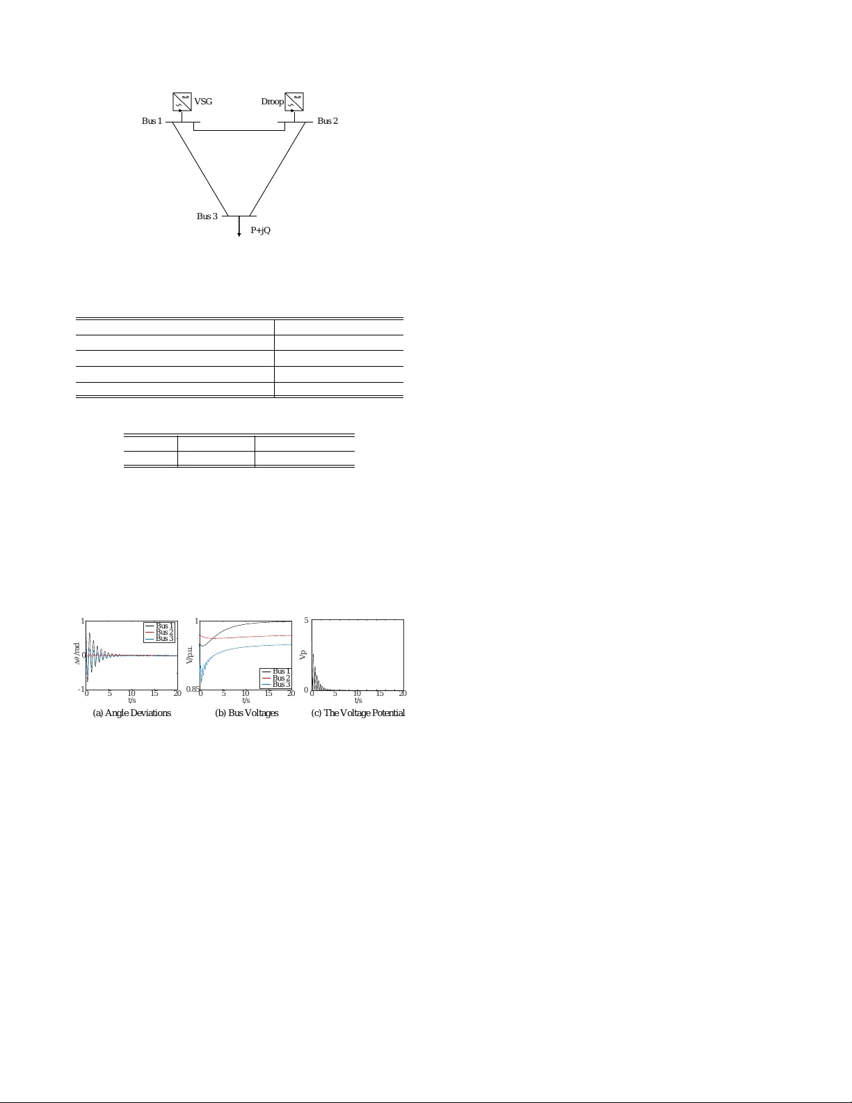
T owards Distrib uted Stability Analytics of Dynamic P ower Systems: A Phasor -Cir cuit Theory P erspectiv e Peng Y ang 1 , Feng Liu 1 , Zhaojian W ang 1 , Shicong Ma 2 1. Department of Electrical Engineering, Tsinghua Univ ersity , Beijing 100084, China E-mail: lfeng@tsinghua.edu.cn 2. China Electric Power Research Institute, Beijing 100192, China E-mail: mashicong@epri.sgcc.com.cn Abstract: W ith the rapid dev elopment of renewable and distributed energies, the underlying dynamics of power systems are no longer dominated by large synchronous generators, but by numerous dynamic components with heterogeneous characteristics. In such a situation, the traditional stability analysis method may fail due to the challenges of heterogeneity and scalability . In this paper , we handle this issue by fundamental circuit theory . Inspired by the work of Brayton and Moser in the nonlinear RLC circuit, we extend the concept of the voltage potential to phasor circuits and offer new results into the distributed stability analytics in power systems. W e show that under certain distrib uted passivity-lik e conditions the system-wide stability can be ensured. The simulation of a 3-bus system is also pro vided to verify our results. Key W ords: Power Systems Stability , Distrib uted Stability Criterion, Phasor-Circuit Theory , Con vexity , P assivity . 1 Introduction Stability is the primary concern in power systems. In re- cent years, howe ver , with the rapid development of rene wable energies and distributed energy technologies, the underlying dynamics of power systems are changing and deterioration of system-wide stability has been witnessed [1, 2]. T raditionally , the stability analysis only in v olves the dynam- ics of synchronous machines and is carried out in a centralized manner [3]. These center-based methods may fail since the dynamics of the po wer system will be no longer dominated by similar synchronous machines but most-likely consists of numerous heterogeneous dynamic components [4]. The chal- lenges under such a circumstance are mainly two folds: het- erogeneity and scalability . This motiv ates distributed stability analytic methods which adapt to heterogeneous components’ models and can be carried out distributedly while guarantee- ing the system-wide stability . Many ef forts ha ve been putting into this task recently . Meth- ods based on distributed analysis of the Jacobian matrix [5 – 7] and the transfer function [8, 9] have been proposed. These methods can analyze the small-signal stability of the intercon- nected system in by distributed conditions. Another approach is based on the concept of passivity or dissipativity [10–12]. In this approach, the system-wide stability is induced as long as each component meets certain passivity condition. The biggest challenge in this approach is to find the right passi vity condi- tion to minimize its conservati veness and improve its appli- cability while maintaining the system-wide stability . In ad- dition, methods based on linear matrix inequalities[13], sum- of-square technique and vector L yapunov functions [14] are also proposed. These computation-based methods decompose the task of system-wide stability assessment into se veral dis- This work is supported by the project ”Research on The Change of Sta- bility Characteristics in Po wer Systems with High Renewable Energy Penetra- tion”. tributed calculations. The aforementioned methods, howe ver , are still insufficient to meet the urgent requirement in hetero- geneous scalable power systems, since they either limit to the small-signal stability or suf fer from the computational burden. In this paper , we turn to fundamental circuit theories and present another perspective to handle the issue of distributed stability with concerns about heterogeneity and scalability . As we only concern the dynamics near the nominal frequency , the A C po wer system can be reg arded as a circuit in the sinusoidal quasi-steady state [3] and is essentially a phasor circuit as de- fined in this paper . W e extend the idea of Brayton and Moser [15, 16] , which was first proposed in 1964 to analyze the sta- bility of topologically complete nonlinear RLC circuits, to a class of phasor circuit with special applications to power sys- tems. W e first define the voltage potential of the phasor circuit following the line in [15]. Then we explore its properties with mathematical tools in complex analysis and dynamic systems. Based on that, we provide a passi vity-like condition for each component to guarantee the system-wide stability in power systems. Due to the space limit, we present sev eral claims without proof in this paper . The rest of this paper is organized as follows. Section 2 introduces some basic concepts and formulates the problem; the voltage potential of the phasor circuit is defined and ana- lyzed in Section 3; the distributed stability issue is addressed in Section 4; a numerical example is illustrated in Section 5; and Section 6 concludes this paper . Notations: j is the imaginary unit; R and C are the sets of real and complex numbers, respecti vely; R ≥ 0 is the set of non- negati ve real numbers; superscript ∗ is the complex conjugate; col ( x 1 , x 2 ) is a column vector with entries x 1 and x 2 ; 0 n ∈ R n denotes a vector with all zeros entries; for x ∈ C , Im x and Re x stand for the imaginary and the real part of x , respectiv ely . 2 Problem F ormulation 2.1 Phasor Representation of P ower Systems Consider a symmetric AC three-phase po wer system. Elec- trical quantities in such a system hav e the following form. Definition 1. [17] A function of time x abc : R ≥ 0 → R 3 is called a symmetric A C three-phase signal if it is described by x abc ( t ) =   x a ( t ) x b ( t ) x c ( t )   = A ( t )   sin( θ ( t )) sin( θ ( t ) − 2 π 3 ) sin( θ ( t ) + 2 π 3 )   (1) where A : R ≥ 0 → R ≥ 0 is called the amplitude and θ : R ≥ 0 → R is called the phase angle. Note that both the amplitude and phase angle may change with time. For the simplicity of notations, we will omit the time argument whene ver it is clear in the context. Due to the symmetry in (1), a coordinate transformation, known as the dq 0 -transformation, is introduced to simplify the analysis. Definition 2. [18] Let x : R ≥ 0 → R 3 and φ : R ≥ 0 → R . Consider the matrix function T dq 0 : R → R 3 × 3 T dq 0 ( φ ) = r 2 3   cos( φ ) cos( φ − 2 π 3 ) cos( φ + 2 π 3 ) sin( φ ) sin( φ − 2 π 3 ) sin( φ + 2 π 3 ) √ 2 2 √ 2 2 √ 2 2   Then, the mapping f dq 0 : R 3 × R → R 3 f dq 0 ( x ( t ) , φ ( t )) = T dq 0 ( φ ) x ( t ) (2) is called the dq 0 -transformation. Apply the dq 0 -transformation to the symmetric AC three- phase signal x abc yields x dq 0 =   x d x q x 0   = T dq 0 ( φ ) x abc = r 3 2 A   sin( θ − φ ) cos( θ − φ ) 0   (3) Since x 0 ( t ) ≡ 0 , a symmetric A C three-phase signal is totally dictated by its dq components as follows. x dq =  x d x q  = r 3 2 A  sin( θ − φ ) cos( θ − φ )  (4) Let a complex number ¯ X = q 3 2 Ae j ( θ − φ ) . It follo ws that ¯ X = x q + j x d (5) W e call it the phasor representation of x abc and refer ¯ X as a phasor , which is defined rigorously as follows. Definition 3. A function of time ¯ X : R ≥ 0 → C is called a phasor if it is described by ¯ X ( t ) = X ( t ) e j φ ( t ) (6) where X : R ≥ 0 → R ≥ 0 is called the magnitude and φ : R ≥ 0 → R is called the phase angle. W e also denote ¯ X ( t ) := X ( t ) ∠ φ ( t ) . Remark 1. Our definition of phasor follo ws the line in [19], where the magnitude and angle are both functions of time. Note, howe ver , in the study of the sinusoidal steady-state cir- cuit, a phasor usually means a constant complex number . It has been sho wn in [18] that the dynamic state variables of a symmetric A C three-phase power system can be ex- pressed as phasors via time-scale separation. This justifies all phasor-based dynamic models for po wer system stability anal- ysis, such as the well-known network-reduction and network- preserving model [20]. 2.2 Po wer Systems as Phasor Circuits Consider a power system represented in the phasor coordi- nate as introduced previously . W e now show that such a system can be regarded as a circuit with phasor electrical quantities which we call a phasor cir cuit in this paper . The symmetric AC three-phase power system can be ab- stracted as a directed graph G = ( V , E ) , where V is the set of nodes and E is the set of branches. Each branch stands for a symmetric three-phase component in the power system. As- sume graph G has b branches and n nodes. Among all nodes, one specific node corresponds to the gr ound which serves as a magnitude reference. Each branch µ ∈ E is associated with a symmetric AC three-phase voltage v µ abc and current i µ abc , as well as their phasor representation ¯ V µ and ¯ I µ . W e assume the voltages and currents take the associated reference direction 1 endowed by G . As components are interconnected electrically , their volt- ages and currents are constrained by the Kirchhoff ’ s current law (KCL) and the Kirchhof f ’ s voltage la w (KVL) as follows. X node ± i µ abc = 0 3 , X loop ± v µ abc = 0 3 (7) where ± means that the signal takes proper sign accordingly . Proposition 1. Consider a symmetric A C three-phase power system G = ( V , E ) . If the dq 0 -transformation (2) with a uni- form φ ( t ) is applied to each symmetric A C three-phase line current i µ abc and voltage v µ abc , then the corresponding phasors ¯ I µ and ¯ V µ satisfy the following KCL and KVL. X node ± ¯ I µ = 0 , X loop ± ¯ V µ = 0 (8) Pr oof. Clearly with a uniform φ ( t ) we hav e X ± x µ dq 0 = X ± T dq 0 ( φ ) x µ abc = T dq 0 ( φ ) X ± x µ abc = 0 3 which completes the proof. It shows that if the dq 0 -transformation with a uniform φ is applied to the po wer system, then the system can be regarded as a phasor circuit. That means the power system is essen- tially a graph G = ( V , E ) with branch currents and voltages as 1 The associated reference direction means that positiv e current is defined as flowing into the terminal which is defined to have positiv e voltage. Note that these directions may be different from the direction of the actual current flow and v oltage. phasors and obeys the fundamental KCL and KVL. In the asso- ciated reference direction, the inner product of branch voltage phasor and negativ e current phasor defines the complex power generation in the corresponding branch, S µ = − ¯ I ∗ µ ¯ V µ = P µ + j Q µ (9) where P µ and Q µ are the active and reactiv e power generated in branch µ , respectiv ely . A component in the power system is abstracted as a branch in G , which determines the relation between ¯ V µ and ¯ I µ locally . W e assume that the power system consists of dynamic voltage sources/loads, transmission lines, and constant power loads. All these components can be divided into two kinds: the static and the dynamic. W e denote the set of branches associated with static and dynamic components by S and D , respecti vely . W e have E = S ∪ D . The static component establishes a mapping between ¯ V µ and ¯ I µ , which is also called the voltage-current characteristic in the context of circuit theories. The static component can be generically modeled as g µ ( ¯ V µ , ¯ I µ ) = 0 (10) In this paper, we consider two kinds of static component in a power system. One is the linear admittance y µ which is used to model the transmission line in a power system [3]. It giv es a static relation as ¯ I µ − y µ ¯ V µ = 0 (11) The other is the constant power source/load ¯ I ∗ µ ¯ V µ − P 0 µ − j Q 0 µ = 0 (12) Denote the sets of these two type branches by S 1 and S 2 . The dynamic component relates ¯ V µ and ¯ I µ by differential equations. W e consider a generic model for the dynamic com- ponent as follows. ˙ x µ = f µ ( x µ , u µ ) (13) where x µ = col ( ξ µ , V µ , θ µ ) ∈ X µ × R > 0 × R is the state variable of dynamic component µ , and ξ µ ∈ X µ is the auxil- iary state v ariable which includes the heterogeneous dynamics of each component. The input is the power generation in the branch u µ = ( P µ , Q µ ) ∈ R 2 . f µ : X µ × R > 0 × R 3 → X µ × R > 0 × R is a continuously dif ferentiable function. Not- ing that ¯ I µ = − ( P µ + j Q µ V µ ) ∗ , component (13) determines a dy- namic relation between ¯ V µ and ¯ I µ . In a power system, the generic formulation (13) can repre- sent a wide variety of dynamics, such as the synchronous ma- chine [3], the inv erter-interfaced power source in grid-feeding mode [18], and loads with frequency and voltage response [10]. T o state our results, we make the follo wing assumption on the circuit topology of a power system. Assumption 1. The graph of the circuit is connected. And all dynamic branches ha ve one end connecting to the ground, i.e., they are connected to the po wer system in a parallel fashion. Assumption 1 is usually true for a power system since gen- erators and loads are usually connected to the ground. Combining all components’ relations and the circuit inter- connection constrain, the entire phasor circuit can be modeled by a set of differential algebraic equations (D AEs) as follo ws.          ˙ x µ = f µ ( x µ , u µ ) , µ ∈ D 0 = g µ ( ¯ V µ , ¯ I µ ) , µ ∈ S 0 = X node ± ¯ I µ , 0 = X loop ± ¯ V µ (14) Assumption 2. The D AEs (14) of a phasor circuit is of index-1 [21]. Assumption 2 is very common in the study of network- preserving po wer system model [20]. It ensures the mapping from the state variables to algebraic is one-to-one locally . 3 V oltage P otential of Phasor Circuits Consider a phasor circuit G . The set of branch voltages ¯ V = ( ¯ V 1 , ¯ V 2 , . . . , ¯ V b ) and the set of branch currents ¯ I = ( ¯ I 1 , ¯ I 2 , . . . , ¯ I b ) are vectors in C b . The KCL and the KVL of phasor circuits (8) put a linear constrain to the domain of ¯ I and ¯ V . Denote I and V as two subsets of C b such that ev ery ¯ I ∈ I and ¯ V ∈ V satisfies (8). W e have both I and V are subspaces of C b as (8) are linear . Define the inner product of two vectors in x, y ∈ C b as < x, y > = P b µ =1 xy ∗ . Follo wing the lines in [15, Therome 1] and [15, Therome 2], we have following two lemmas. Lemma 2. If ¯ I ∈ I and ¯ V ∈ V , then < ¯ V , ¯ I > = 0 , i.e. V ⊥ I . Lemma 3. Let Γ be a one-dimensional curve in C b , then we hav e Z Γ X µ ∈V ¯ I ∗ µ d ¯ V µ = 0 3.1 Line Integral of Static Components Now consider the phasor circuit composes of static and dy- namic components introduced in Section 2.2. By Assumption 2, the voltages and currents of all static network branches are determined by the voltages of dynamic branches. So we can specifically choose Γ from a fixed point in C b to a variable one in such a manner that Γ is a solution trajectory of (14). Along this Γ , we hav e Z Γ ¯ I ∗ µ d ¯ V µ = Z Γ y ∗ µ ¯ V ∗ µ d ¯ V µ , ∀ µ ∈ S 1 (15) As this comple x function clearly violates the Cauchy-Riemann equations, the above line integral is path-dependent [22]. How- ev er , Inspecting the real and imaginary part of this inte gral sep- arately , we ha ve the following proposition. Proposition 4. The real part of (15) is path-independent if and only if Im y µ = 0 . And the imaginary part of (15) is path- independent if and only if Re y µ = 0 . Pr oof. Denote y µ = g µ + j b µ and ¯ V µ = x + j y . Consider the imaginary part of (15) as an example. Im Z Γ y ∗ µ ¯ V ∗ µ d ¯ V µ = Im Z Γ ( g µ − j b µ )( x − j y ) d ( x + j y ) = Z Γ ( − b µ x − g µ y ) dx + ( g µ x − b µ y ) dy (16) By Green’ s theorem, the integral above is path-independent if and only if ∂ ( g µ x − b µ y ) ∂ x = ∂ ( − b µ x − g µ y ) ∂ y ⇔ g µ = − g µ ⇔ g µ = 0 Similarly , we can prove that the real part of (15) is path- independent if and only if all b µ = 0 . Remark 2. In the context of the power system, the preceding proposition states that the integral (16) is path-independent if and only if we ne glect all the transfer conductances or the sus- ceptances in the network. Since the integral (16) is related to the energy function in the transient stability analysis of power systems [23], the claim here is consistent with the common be- lief that the existence of non-zero transfer conductances leads to path-dependent term in energy functions. Assumption 3. W e assume the transmission lines in the power system are lossless, i.e. g µ = 0 , ∀ µ ∈ S 1 . Under this assumption, we hav e X µ ∈S 1 Im Z Γ ¯ I ∗ µ d ¯ V µ = X µ ∈S 1 Z Γ ( − b µ x ) dx + ( − b µ y ) dy = X µ ∈S 1 − 1 2 b µ ( x 2 + y 2 )    Γ = X µ ∈S 1 − 1 2 b µ | ¯ V µ | 2    Γ (17) which equals half of reactiv e power in the transmission lines. For constant po wer component, by (9) we have Im Z Γ ¯ I ∗ µ d ¯ V µ = − Im Z Γ P 0 µ + j Q 0 µ ¯ V µ d ¯ V µ , ∀ µ ∈ S 2 (18) The line integral is path-independent and if we denote ¯ V µ = V µ ∠ θ µ , the integral can be e xpress as Im Z Γ ¯ I ∗ µ d ¯ V µ = − P 0 µ θ µ − Q 0 µ ln V µ    Γ (19) Now we are ready to define the v oltage potential of a phasor circuit. Definition 4. Consider a phasor circuit satisfying Assumption 3. The function V p : C b → R is called the voltage potential of the phasor circuit. V p ( ¯ V ) = X µ ∈S Im Z Γ ¯ I ∗ µ d ¯ V µ = X µ ∈S 1 − 1 2 b µ | ¯ V µ | 2 − X µ ∈S 2 P 0 µ θ µ − Q 0 µ ln V µ (20) 3.2 Line Integral of Dynamic Components By Assumption 2, the end node of dynamic component µ is the ground. Suppose its non-ground terminal is indexed by i , then we have ¯ V µ = V i ∠ θ i , and P µ and Q µ are identical to the power generated from the node i.e. P µ + j Q µ = P i + j Q i . So for dynamic components, we hav e Im Z Γ ¯ I ∗ µ d ¯ V µ = − Im Z Γ P i + j Q i V i e j θ i d ( V i e j θ i ) = − Z Γ P i dθ i + Q i d ln V i (21) This integral is generally path-dependent and is dictated by dif- ferential equations (13). Now we are ready to present the key observation in this pa- per . The proof is straightforward by inv oking Lemma 3 and is omitted due to space limit. Theorem 5. Consider a phasor circuit (14) satisfying Assump- tion 1-3. For an y solution trajectory γ : R ≥ 0 → C b , we hav e X i ∈D Z γ ( t ) γ (0) P i dθ i + Q i d ln V i = V p ( γ ( t )) − V p ( γ (0)) (22) where V p is the voltage potential of this phasor circuit. 4 Distributed Stability Analytics 4.1 Distributed Criteria f or System-Wide Stability In this section, we propose distributed criteria for system- wide stability based on the voltage potential of phasor circuits. By law of cosines, the modulus of branches voltage can be rewritten in terms of node voltages. Assume ¯ V µ = V i ∠ θ i − V k ∠ θ k , we hav e | ¯ V µ | 2 = V 2 i + V 2 k − 2 V i V k cos θ ik (23) Substituting into (17) yields Im Z Γ ¯ I ∗ µ d ¯ V µ = 1 2 B ik ( V 2 i + V 2 k − 2 V i V k cos θ ik )    Γ (24) where B ik is element in the network admittance matrix and we hav e B ik = − b ik . Let x e := col ( ξ e , V e , θ e ) be an equilibrium of the phasor circuit system (14). For the voltage potential (20), define the initial point ¯ V 0 = V 0 ∠ θ 0 ∈ C b corresponding to x e , 2 New re- sults: it should be the initial point of the line integral, rather than the equilibrium. and formulate in the bus voltage coordi- nate (24) V p ( V , θ ) = X ( i,k ) ∈S 1 1 2 B ik ( V 2 i + V 2 k − 2 V i V k cos θ ik ) − X ( i,k ) ∈S 2 P 0 ik θ ik − Q 0 ik ln V ik (25) Now consider the Bregman diver gence [24] between z := col ( V , θ ) and z 0 := col ( V 0 , θ 0 ) w .r .t. V p as follows. W ( z ) = V p ( z ) − ( z − z 0 ) T ∇ V p ( z 0 ) − V p ( z 0 ) (26) 2 By Assumption 2 all algebraic variables is dictated by state v ariables. W e have W ( z 0 ) = ∇ W ( z 0 ) = 0 and ∇ 2 W ( z ) = ∇ 2 V p ( z ) . Further , the Bregman div ergence induced by V p has the fol- lowing property . Lemma 6. Consider a phasor circuit (14) satisfying Assump- tion 1-3. For an y solution trajectory γ : R ≥ 0 → C b , we hav e X i ∈D Z γ ( t ) γ (0) ∆ P i dθ i + ∆ Q i d ln V i = W ( γ ( t )) − W ( γ (0)) (27) where ∆ P i = P i − P e i , ∆ Q i = Q i − Q e i , and W is the Bregman div ergence induced by the voltage potential V p . Theorem 7. Consider a phasor circuit (14) satisfying Assump- tion 1-3. For an y bounded trajectory γ : R ≥ 0 → C b , if Z γ ( t ) γ (0) ∆ P i dθ i + ∆ Q i d ln V i ≤ 0 , ∀ i ∈ D , ∀ t ∈ R ≥ 0 . (28) and the largest in variant set of { ∆ P i dθ i + ∆ Q i d ln V i = 0 } only contains equilibrium, then the trajectory γ ( t ) will con- ver ge to the set of equilibrium. Since the lar gest in v ariant set condition in Theorem 7 is usu- ally satisfied for power system models [20], Theorem 7 in- dicates that the unstable patterns of bounded trajectory , such as oscillation, can be precluded if every dynamic component obeys the inte gral inequality (28). Consider again the Bre gman diver gence W ( z ) (26). W e de- note the set of equilibrium points which satisfy the con vexity condition E =  x e : ∇ 2 W ( z 0 ) ≥ 0  (29) where the only zero eigenv alue of ∇ 2 W ( z 0 ) comes from the rotational symmetry of phase angles [25]. The following theorem offers a distributed criterion for sta- bility w .r .t. any equilibrium in E . Theorem 8. Consider a phasor circuit (14) satisfying Assump- tion 1-3. For any x e ∈ E , if for all i ∈ D , there exists a continues differentiable scalar function W i ( x i ) such that W i is locally positiv e definite at local equilibrium x e i and satisfies ˙ W i ≤ ∆ P i ˙ θ i + ∆ Q i ˙ ln V i (30) then the system-wide equilibrium x e is stable. Note that in both Theorem 7 and Theorem 8, we do not spec- ify the dynamic models but propose generic criteria which can accommodate to the heterogeneity . Moreover , our criteria in- volv e only local information as shown in (28) and (30). Thus, it can be employed and assessed individually which fulfills the scalability requirement. Remark 3. Compared to the classical passi vity condition [26] , the left-hand side of (30) can be regarded as a supply rate, in which the input is (∆ P i , ∆ Q i ) , howe ver , the output is time deriv ativ es ( ˙ θ , ˙ ln V ) . Thus, the condition (30) is called a passivity-lik e condition in this paper . Remark 4. The con vexity condition (29) of equilibrium plays an important role in Theorem 8. It guarantees a well-defined distance such that the L yapunov argument can be employed. Roughly speaking, it is satisfied when the load is light. See [27] for more information about under what condition the power system satisfies (29). 4.2 Examples of Dynamic Components In this section, we giv e two specific examples of dynamic components and demonstrate ho w they meet the criterion in Theorem 8. W e first consider the inv erter-interfaced renewable energy sources which are controlled by the virtual synchronous gen- erator (VSG) technique [28] as follows.      ˙ θ i = ω i M i ˙ ω i = − D p i ω i + P e i − P i τ q i ˙ V i = − ( V i − V e i ) − D q i ( Q i − Q e i ) (31) where D p i is the droop coefficient, τ q i is the time constant, M i is the virtual inertial, and the superscript e stands for the equi- librium value. T o meet the criterion in Theorem 8, one can choose W i ( x i ) = 1 2 M i ω 2 i + k i D q i  V i V e i − ln V i  (32) where k i = V e i + D q i Q e i is a constant. One can verify that con- dition (30) holds and x e i = col (0 , V e i , θ e i ) is a local minimum of (32) when k i > 0 . Another example is the in verter -interfaced component with the droop controller [7] as follows. ( τ p i ˙ θ i = − ( θ i − θ e i ) − D p i ( P i − P e i ) τ q i ˙ V i = − ( V i − V e i ) − D q i ( Q i − Q e i ) (33) where D p i , D q i are droop coef ficients, τ p i , τ q i are time constants, and the superscript e stands for the equilibrium value. T o meet the criterion in Theorem 8, similarly one can choose W i ( x i ) = ( θ i − θ e i ) 2 2 D p i + k i D q i  V i V e i − ln V i  (34) where k i = V e i + D q i Q e i and one can verify that condition (30) holds and x e i = col ( V e i , θ e i ) is a local minimum of (34) when k i > 0 . 5 Case Study Consider a 3-bus power system as showed in Figure 1. Bus 1 and 2 are attached to a VSG (31) and a droop controlled (33) in verter source, respectiv ely . Bus 3 is connected to a constant power load P 0 3 + j Q 0 3 . The parameters and equilibrium of the system are listed in T able 1 and T able 2. One can verify that the equilibrium satisfies the conv exity condition (29). And both dynamic components meet the crite- rion in Theorem 8 with the giv en parameters. Thus, by Theo- rem 8, it follows that the interconnected power system should be stable. B us 1 B us 2 B us 3 V S G D r oop P + j Q Fig. 1: The schematic of the 3-bus system. T able 1: System Parameters Line Reactance 0.12 V irtual Inertial M 1 0.16 Droop Coefficients D p 1 , D q 1 , D p 2 , D q 2 0.076, 0.03, 0.02, 0.02 T ime Constants τ q 1 , τ p 2 , τ q 2 0.3, 6.56, 8 Load Profile P 0 3 , Q 0 3 0.03, 0.55 T able 2: System Equilibrium V e 1 ∠ θ e 1 V e 2 ∠ θ e 2 V e 3 ∠ θ e 3 1 ∠ 0 0 . 97 ∠ 0 . 001 0 . 95 ∠ − 0 . 0015 T o verify the theoretical result, suppose the system encoun- ters a fault and undergoes a transient process. The dynamic response is showed in Figure 2 (a) and (b). The system is sta- ble which is consistent with our claim. The voltage potential V p (20) is also depicted in Figure 2 (c). It is clear that V p tends to zero as the system con verges to the stable equilibrium. ( a ) A ngl e D e vi a t i on s ( c ) T he V ol t a ge P ot e nt i a l ( b ) Bus V ol t a ge s 0 5 10 15 20 t / s - 1 0 1 / ra d   Bus 3 Bus 2 Bus 1 0 5 10 15 20 t / s V / p . u . Bus 3 Bus 2 Bus 1 0 5 10 15 20 t / s V p 0 . 85 1 0 5 Fig. 2: (a) The angle de viations, (b) the v oltage de viations, and (c) the voltage potential during the transient process. 6 Concluding Remarks W e hav e presented a phasor-circuit theory perspectiv e to handle the stability issue of po wer systems. Based on the ob- servation that the symmetric AC three-phase power system can be regarded as a phasor circuit, we have extended and studied the concept of voltage potential with mathematical tools from complex analysis. Our results sho w that under the con vexity condition, the system-wide stability can be ensured if each dy- namic component meets a passivity-like condition, which can fit heterogeneous models and is scalable. In future works, we will relax the con vexity condition and enlarge the v alid scope of our criteria. W e belie ve that when the power system becomes more complex, in order to handle its stability issues, it is helpful or even necessary to revie w some basic circuit theories. References [1] Meegahapola, Lasantha, and Damian Flynn. ”Impact on transient and frequency stability for a po wer system at very high wind pen- etration. ” IEEE PES General Meeting . IEEE, 2010. pp. 1-8. [2] An, Zhi, et al. ”Analysis on Sub-Synchronous Oscillation Asso- ciated with Wind Farms Based on Direct-Driven W ind Genera- tors. ” 2018 37th Chinese Control Conference . IEEE, 2018. pp. 1282-1286. [3] Kundur , Prabha, Neal J. Balu, and Mark G. Lauby . P ower system stability and contr ol . V ol. 7. New Y ork: McGraw-hill, 1994. [4] Farhangi, Hassan. ”The path of the smart grid. ” IEEE P ower and Ener gy Magazine 8.1 (2010): 18-28. [5] Y . Song, D. J. Hill, T . Liu, and Y . Zheng. ”A Distributed Frame- work for Stability Ev aluation and Enhancement of Inv erter-Based Microgrids. ” IEEE T rans. Smart Grid , vol. 8, no. 6, pp. 3020- 3034, Nov . 2017. [6] M. D. Ili ´ c and Q. Liu. ”T ow ard standards for model-based control of dynamic interactions in lar ge electric power grids. ” in Pr oceed- ings of The 2012 Asia P acific Signal and Information Pr ocessing Association Annual Summit and Confer ence , 2012, pp. 1-8. [7] Y . Zhang and L. Xie. ”Online Dynamic Security Assessment of Microgrid Interconnections in Smart Distribution Systems. ” IEEE T rans. P ower Syst. , vol. 30, no. 6, pp. 3246-3254, Nov . 2015. [8] Pates, Richard, and Enrique Mallada. ”Rob ust Scale-Free Syn- thesis for Frequency Control in Power Systems. ” arXiv pr eprint arXiv:1804.00729 . 2018. [9] R. Pates and E. Mallada. ”Decentralised Robust In verter-based Control in Power Systems. ” IF A C-P aper sOnLine , vol. 50, no. 1, pp. 5548-5553, Jul. 2017. [10] A. Kasis, E. Dev ane, C. Spanias, and I. Lestas. ”Primary Fre- quency Regulation W ith Load-Side ParticipationPart I: Stability and Optimality . ” IEEE T rans. P ower Syst. , vol. 32, no. 5, pp. 3505-3518, Sep. 2017. [11] C. Spanias and I. Lestas. ”A System Reference Frame Approach for Stability Analysis and Control of Power Grids. ” IEEE T rans. P ower Syst. . v ol. 34, no. 2, pp. 1105-1115, Mar . 2019. [12] S. Y . Caliskan and P . T ab uada. ”Compositional T ransient Sta- bility Analysis of Multimachine Po wer Networks. ” IEEE T rans. Contr ol Network Syst. , vol. 1, no. 1, pp. 4-14, Mar . 2014. [13] Y . Zhang and L. Xie. ”A T ransient Stability Assessment Frame- work in Power Electronic-Interfaced Distribution Systems. ” IEEE T rans. P ower Syst. , vol. 31, no. 6, pp. 5106-5114, Nov . 2016. [14] S. Kundu and M. Anghel. ”A sum-of-squares approach to the stability and control of interconnected systems using vector L ya- punov functions. ” in 2015 American Control Conference, 2015, pp. 5022-5028. [15] R. K. Brayton and J. K. Moser . ”A theory of nonlinear networks. I. ” Quart. Appl. Math. , v ol. 22, no. 1, pp. 1-33, 1964. [16] R. K. Brayton and J. K. Moser . ”A theory of nonlinear networks. II. ” Quart. Appl. Math. , v ol. 22, no. 2, pp. 81-104, 1964. [17] Akagi, Hirofumi, Edson Hirokazu W atanabe, and Mauricio Are- des. Instantaneous power theory and applications to power con- ditioning . V ol. 62. John Wile y & Sons, 2017. [18] J. Schif fer, D. Zonetti, R. Orte ga, A. M. Stanko vi, T . Sezi, and J. Raisch. ”A surve y on modeling of microgridsFrom fundamental physics to phasors and voltage sources. ” Automatica , vol. 74, pp. 135-150, Dec. 2016. [19] Zhong, Qing-Chang, and T omas Hornik. Contr ol of power in- verters in renewable energy and smart grid inte gration . V ol. 97. John W iley & Sons, 2012. [20] Z. W ang, F . Liu, J. Z. F . Pang, S. H. Low , and S. Mei. ”Dis- tributed Optimal Frequency Control Considering a Nonlinear Network-Preserving Model. ” IEEE T rans. P ower Syst. , vol. 34, no. 1, pp. 76-86, Jan. 2019. [21] P . Kunk el and V . Mehrmann. Differ ential-algebraic Equations: Analysis and Numerical Solution. European Mathematical Soci- ety , 2006. [22] L. V . Ahlfors. Complex analysis: an intr oduction to the theory of analytic functions of one complex variable . McGraw-Hill, 1979. [23] Y .H. Moon, B.H. Cho, Y .H. Lee, and H.J. Kook. ”Deri vation of energy conservation law by complex line integral for the direct energy method of power system stability . ” in Pr oceedings of the 38th IEEE Conference on Decision and Contr ol , 1999, v ol. 5, pp. 4662-4667 vol.5. [24] J. W . Simpson-Porco. ”Equilibrium-Independent Dissipativity W ith Quadratic Supply Rates. ” IEEE T rans. Autom. Contr ol , v ol. 64, no. 4, pp. 1440-1455, Apr . 2019. [25] F . D ¨ orfler , M. Chertko v , and F . Bullo. ”Synchronization in com- plex oscillator networks and smart grids. ” PNAS , vol. 110, no. 6, pp. 2005-2010, Feb . 2013. [26] A. van der Schaft. L2-Gain and P assivity T echniques in Nonlin- ear Contr ol . Cham: Springer International Publishing, 2017. [27] K. Dvijotham and M. Chertkov . ”Con vexity of structure preserv- ing ener gy functions in power transmission: Novel results and applications. ” in 2015 American Contr ol Confer ence , 2015, pp. 5035-5042. [28] Q. Zhong and G. W eiss. ”Synchron verters: In verters That Mimic Synchronous Generators. ” IEEE T rans. Industrial Elec- tr onics . vol. 58, no. 4, pp. 1259-1267, April 2011.