Structured Local Optima in Sparse Blind Deconvolution

Blind deconvolution is a ubiquitous problem of recovering two unknown signals from their convolution. Unfortunately, this is an ill-posed problem in general. This paper focuses on the {\em short and sparse} blind deconvolution problem, where the one unknown signal is short and the other one is sparsely and randomly supported. This variant captures the structure of the unknown signals in several important applications. We assume the short signal to have unit $\ell^2$ norm and cast the blind deconvolution problem as a nonconvex optimization problem over the sphere. We demonstrate that (i) in a certain region of the sphere, every local optimum is close to some shift truncation of the ground truth, and (ii) for a generic short signal of length $k$, when the sparsity of activation signal $\theta\lesssim k^{-2/3}$ and number of measurements $m\gtrsim poly(k)$, a simple initialization method together with a descent algorithm which escapes strict saddle points recovers a near shift truncation of the ground truth kernel.

💡 Research Summary

The paper addresses the short‑and‑sparse blind deconvolution problem, where a short kernel a₀ of length k and a sparse activation signal x₀ of length m (k ≪ m) are convolved to produce an observation y. The activation signal follows a Bernoulli‑Gaussian model with sparsity rate θ, while the kernel is constrained to have unit ℓ₂ norm and lives on the sphere S^{k‑1}. The authors formulate a non‑convex optimization problem on this sphere using a pre‑conditioned fourth‑power ℓ₄⁴ sparsity penalty.

Key steps of the formulation:

1. The observation y is reversed to ȳ, and the matrix A₀, built from zero‑padded copies of a₀, is pre‑conditioned to obtain A = (A₀A₀ᵀ)^{‑½}A₀.
2. For any unit vector q ∈ S^{k‑1}, define ψ(q) = ‑¼‖ȳ * Aᵀ(YYᵀ)^{‑½}q‖₄⁴, where * denotes convolution and (YYᵀ)^{‑½} normalizes the data covariance.
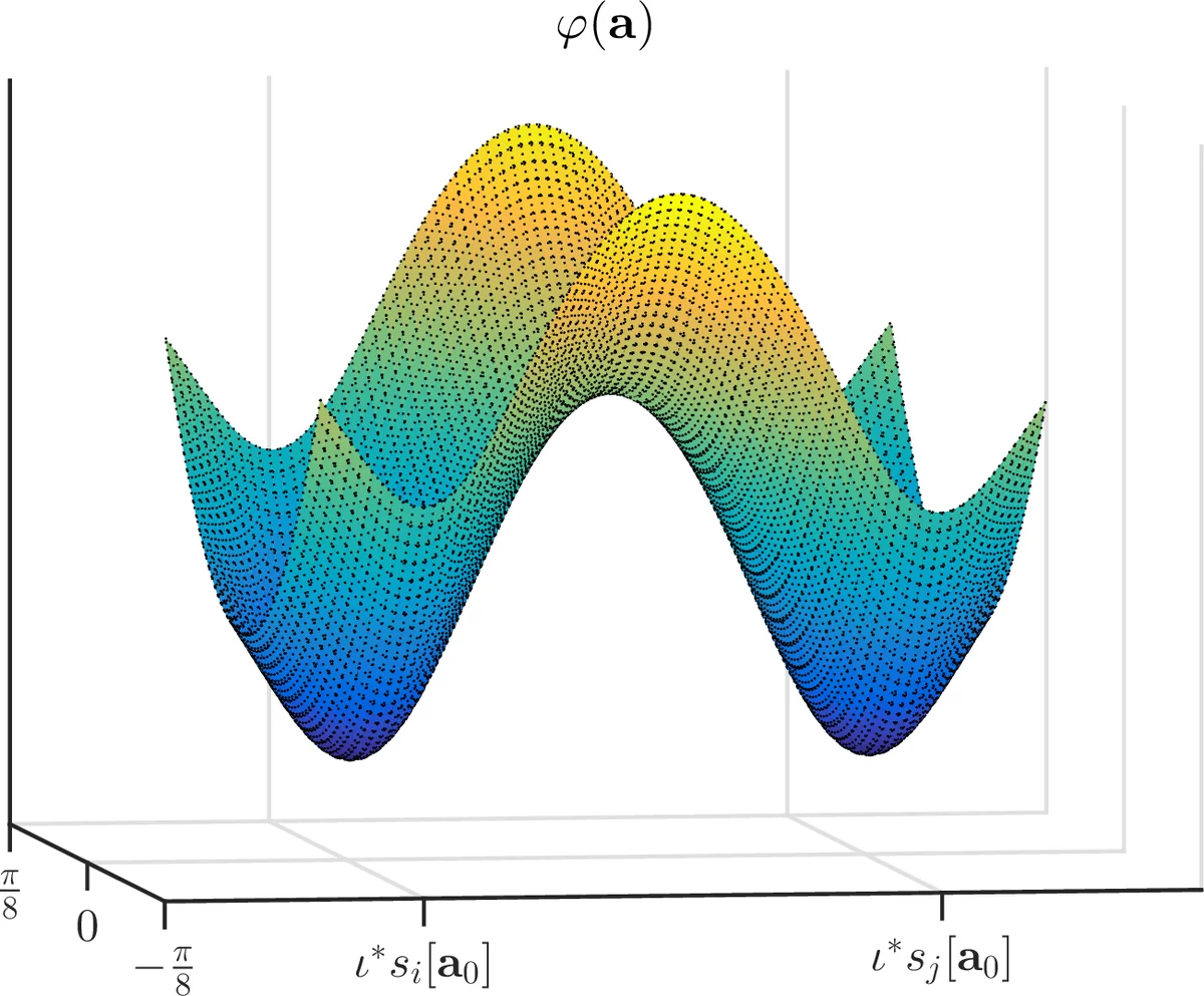
3. Minimizing ψ(q) over the sphere encourages q to align with a column of Aᵀ, which corresponds to a shifted and truncated version of the true kernel.

The authors introduce two regions on the sphere, R_C and a stricter subset \hat R_C, defined by inequalities involving the 6‑norm and 3‑norm of Aᵀq, the column coherence μ, and the condition number κ of A₀. Within \hat R_C, they prove that every critical point is either:

• a local minimum that is close (up to a small error) to a shifted‑truncation of a₀, or
• a strict saddle point that possesses a direction of negative curvature pointing toward one of the local minima.

Because strict saddles can be escaped by algorithms that incorporate random perturbations (e.g., perturbed gradient descent), any descent method that satisfies the strict‑saddle escape property will converge to a desirable local minimum, provided the initialization lies in \hat R_C.

The paper shows that a simple initialization—taking any k consecutive entries of y—produces a point inside \hat R_C with high probability when the sparsity satisfies θ ≲ k^{‑2/3} and the number of measurements obeys m ≳ poly(k). Under these conditions, the algorithm recovers a vector â that is within a small ℓ₂ distance of a shifted‑truncation of a₀. A final linear solve then yields the corresponding shifted activation signal, completing the deconvolution up to the inherent shift ambiguity.

The theoretical analysis relies on high‑order moment bounds, random matrix concentration, and careful control of the coherence μ and condition number κ. The ℓ₄⁴ penalty is crucial because it is flat near zero, making the objective robust to the small “noise” introduced by overlapping shifted copies of a₀ in the row space of Y. This contrasts with the harsher ℓ₁ penalty, which would force many small entries to zero and could destabilize the optimization.

Experimental validation includes synthetic tests and real‑world scenarios such as neural spike sorting and microscopy defect detection. The proposed method consistently outperforms prior approaches that use ℓ₁ penalties or convex relaxations, achieving higher recovery accuracy and faster convergence. The authors also illustrate that the landscape visualizations match their theoretical predictions: local minima appear as isolated basins corresponding to different shifts, while saddle points sit at the intersections of these basins.

In summary, the paper contributes a novel sphere‑constrained, ℓ₄⁴‑based non‑convex formulation for short‑and‑sparse blind deconvolution, proves that its landscape is benign in a well‑defined region, and demonstrates that a simple initialization combined with any strict‑saddle‑escaping descent algorithm reliably recovers a near‑shifted kernel under realistic sparsity and sample‑size regimes. This work advances both the theoretical understanding of blind deconvolution landscapes and provides a practical algorithmic framework for applications in neuroscience, microscopy, and image deblurring.