Integrating the Data Augmentation Scheme with Various Classifiers for Acoustic Scene Modeling

This technical report describes the IOA team’s submission for TASK1A of DCASE2019 challenge. Our acoustic scene classification (ASC) system adopts a data augmentation scheme employing generative adversary networks. Two major classifiers, 1D deep convolutional neural network integrated with scalogram features and 2D fully convolutional neural network integrated with Mel filter bank features, are deployed in the scheme. Other approaches, such as adversary city adaptation, temporal module based on discrete cosine transform and hybrid architectures, have been developed for further fusion. The results of our experiments indicates that the final fusion systems A-D could achieve an accuracy higher than 85% on the officially provided fold 1 evaluation dataset.

💡 Research Summary

The paper presents the IOA team’s solution to the DCASE2019 Task 1A acoustic scene classification (ASC) challenge, achieving over 85 % accuracy on the official fold 1 evaluation set. The core of the system is a data‑augmentation pipeline based on generative adversarial networks (GANs) and a set of complementary classifiers that operate on two distinct acoustic representations: mel‑filter‑bank (FBank) features and wavelet‑derived scalograms.

Two GAN variants are explored. The first is a conditional GAN (ACGAN) that receives the scene label as an additional condition; its loss combines a real/fake binary cross‑entropy term with a scene‑classification term, weighted by a factor γ. The second, called CV AE/ACGAN, augments the conditional GAN with an encoder‑decoder (variational auto‑encoder) structure. The encoder is regularized by a Kullback‑Leibler (KL) divergence to force the latent space toward a unit Gaussian, while a reconstruction loss (mean‑square error on a high‑level discriminator feature) ensures that generated samples preserve the fine‑grained structure of real data. Both models are trained on a “sub‑train” split of the data; generated samples are accepted only if they improve the performance of a base classifier on a corresponding “sub‑test” split, thereby preventing the inclusion of low‑quality synthetic data.

Feature extraction follows two parallel paths. For the FBank branch, short‑time Fourier transform (STFT) is computed with 20 ms windows and 40 ms hops, yielding 128 mel filters per frame. Stereo recordings are processed either as left/right channels or as average‑difference (ave‑diff) channels, and delta/delta‑delta coefficients are appended, resulting in tensors of size 500 × 2 × 128 (or 500 × 6 × 768 after augmentation). For the scalogram branch, STFT is performed with 185 ms windows and 555 ms hops, then a bank of 290 wavelet filters (dense at low frequencies, logarithmic at high frequencies) produces a time‑frequency map of size 58 × 2 × 290.

Classification networks are designed specifically for each feature type. The FBank‑FCNN adopts a VGG‑style 10‑layer 2‑D convolutional architecture with small kernels (5 × 5 or 3 × 3), batch normalization, ReLU activations, and dropout. After the convolutional stack, a 1 × 1 convolution reduces the channel dimension to ten, followed by global average pooling and a soft‑max output. The scalogram‑DCNN uses a series of 1‑D convolutions (kernel size 3) interleaved with pooling and dropout, then three fully‑connected layers (each 1024 units) before the final soft‑max. Frame‑wise predictions are accumulated across the 10‑second clip to obtain a segment‑level decision.

To improve robustness to unseen recording cities, an adversarial city‑adaptation branch is added to the scalogram‑DCNN. This branch consists of a gradient‑reversal layer and a shallow two‑layer city classifier; during training the gradient reversal forces the shared convolutional layers to produce city‑invariant representations while still preserving scene discriminability. A temporal module based on the discrete cosine transform (DCT) is also explored. After the final convolution, the feature map is transformed into the DCT domain, and an attention‑style weighting emphasizes frequency bins that are most informative for the scene classification task.

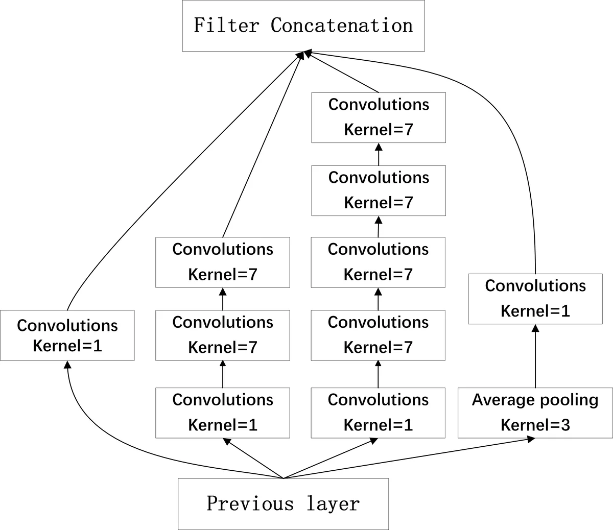
Hybrid network variants are constructed by inserting Inception modules (both 1‑D and 2‑D versions) into the tail of the DCNN and adding parallel recurrent layers (LSTM or GRU). The Inception modules increase receptive field without a large parameter increase, while the recurrent layers aim to capture longer‑range temporal dependencies that pure 1‑D convolutions may miss. Three hybrid configurations are evaluated: IncepLSTM (two Inception‑I modules + two LSTM layers), IncepGRU‑V1 (two Inception‑II modules + two GRU layers), and IncepGRU‑V2/V3 (mixed Inception‑I/II with 2‑D convolutions).

Training follows the official DCASE fold‑1 protocol: the development set is split into training and validation subsets, early stopping is applied if validation loss does not improve for five epochs, and each model is trained with three random seeds to reduce variance. Adam optimizer (β₁ = 0.9, β₂ = 0.999) with an initial learning rate of 1e‑3 is used, and the learning rate is decayed according to validation loss. No external data are employed.

Experimental results show that data augmentation consistently improves all models, with gains ranging from 0.5 % to 4 % absolute accuracy. The CV AE/ACGAN scheme yields a slight additional boost for the scalogram‑DCNN (84.28 % vs. 84.06 % for ACGAN alone). Among single models, the best performer is the scalogram‑avediff‑ACGAN‑DCNN (84.06 %). Adding the DCT temporal module or the adversarial city adaptation raises accuracy to the low‑84 % range, while hybrid Inception‑LSTM/GRU models achieve 83.8 %–83.9 %, slightly below the baseline DCNN. FBank‑based models lag behind, peaking at 80.10 % with ACGAN augmentation.

Ensemble strategies combine the top‑performing models using either simple averaging or weighted voting (weights learned on the fold‑1 validation set). Weighted voting yields marginally higher scores (≈ 0.04 % improvement). Four ensemble configurations (A–D) are reported:

• System A (average voting of seven models) – 85.07 %
• System B (weighted voting of six models) – 85.11 %
• System C (weighted voting of six models, different weight set) – 85.11 %
• System D (weighted voting of eight models) – 85.28 %

The authors conclude that (1) conditional GAN‑based data augmentation is crucial for bridging the domain gap, especially for unseen cities; (2) scalogram features combined with 1‑D DCNNs outperform traditional mel‑filter‑bank FCNNs; (3) adversarial city adaptation and DCT temporal processing provide modest but consistent gains; and (4) a well‑designed ensemble can push performance beyond the 85 % threshold. Future work is suggested to explore more efficient hybrid architectures and stronger domain‑invariant training mechanisms.