Image Super-Resolution Using Attention Based DenseNet with Residual Deconvolution

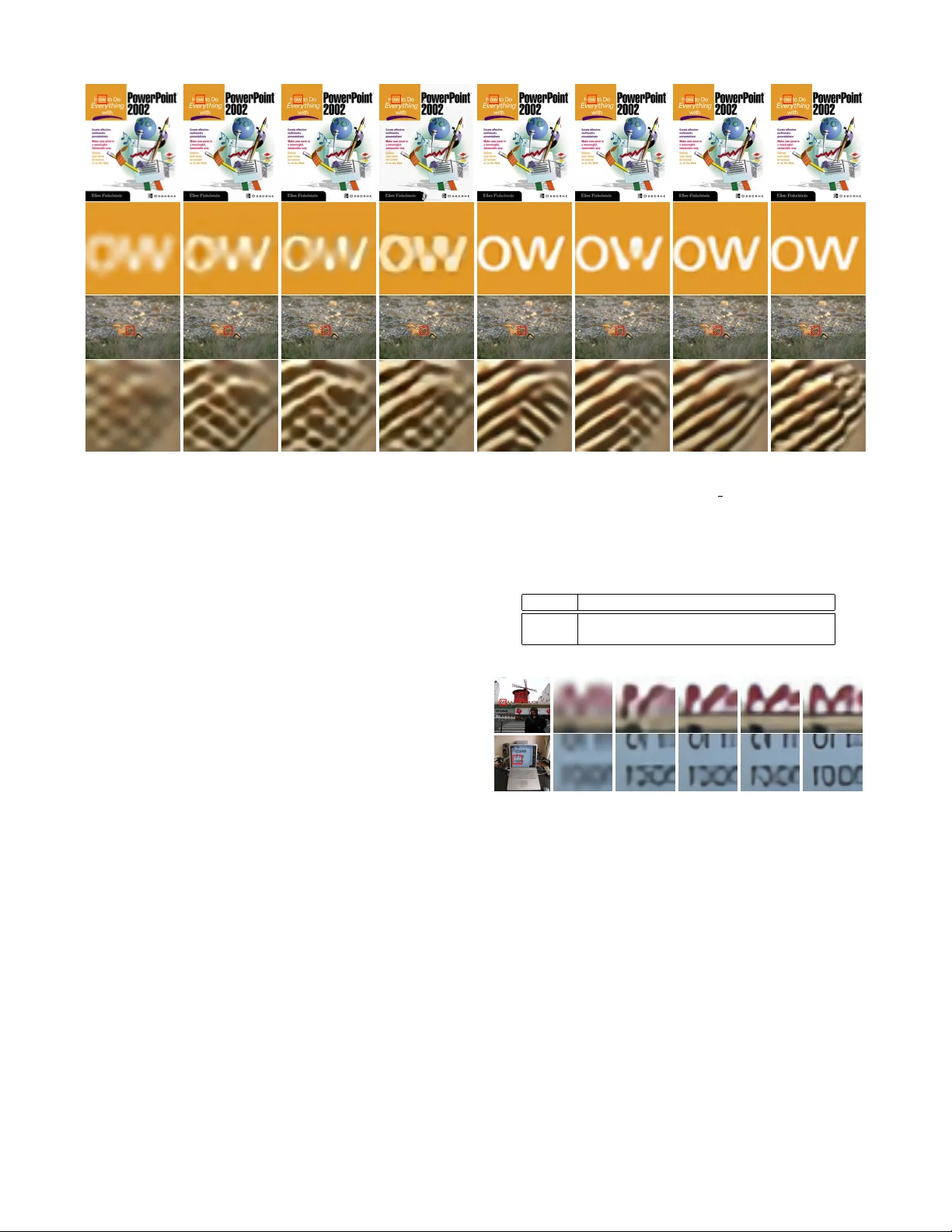
Image Super -Resolution Using Attention Based DenseNet with Residual Decon volution Zhuangzi Li 1 1 Beijing T echnology and Business University lizhuangzii@163.com Abstract Image super-resolution is a challenging task and has attracted increasing attention in research and industrial communities. In this paper , we propose a novel end-to-end Attention-based DenseNet with Residual Deconv olution named as ADRD. In our ADRD, a weighted dense block, in which the cur- rent layer receiv es weighted features from all previ- ous levels, is proposed to capture valuable features rely in dense layers adaptively . And a novel spatial attention module is presented to generate a group of attentive maps for emphasizing informativ e re- gions. In addition, we design an innov ativ e strate gy to upsample residual information via the decon vo- lution layer , so that the high-frequency details can be accurately upsampled. Extensiv e e xperiments conducted on publicly av ailable datasets demon- strate the promising performance of the proposed ADRD against the state-of-the-arts, both quantita- tiv ely and qualitativ ely . 1 Introduction Image super-resolution aims at recovering high-resolution (HR) images from it’ s low-resolution (LR) versions. By far , it has been widely applied to various intelligent im- age processing applications, e.g. license plate recognition [ Liu et al. , 2017 ] , video surveillance [ Zou and Y uen, 2012 ] . Howe ver , image super-resolution is an inherently ill-posed problem since the mapping from the LR to HR space can hav e multiple solutions. T o deal with this issue, various promising super-resolution approaches have been proposed in the past years [ Kim and Kwon, 2010; Y ang et al. , 2013; Freedman and Fattal, 2011; T ai et al. , 2017; Hui et al. , 2018 ] . In image super-resolution, recov ering high-frequency is a key problem that the super -resolved images should be full of edges, textures, and other details. Recently , conv olu- tional neural networks (CNNs) are gradually applied to im- age super-resolution relying on CNN’ s great approximating to capture high-frequency . Dong et al. firstly introduced CNN’ s architecture for the image super-resolution in [ Dong et al. , 2016a ] . Later , a series of CNNs [ Kim et al. , 2016a; Kim et al. , 2016b; T ai et al. , 2017; Lai et al. , 2017; Zhang et al. , 2018 ] try to solve the problem by increasing Bicubic RDN Ours HR Figure 1: Side-by-side image super-resolution comparisons of bicu- bic interpolation, the state-of-the-art RDN, our method and ground- truth HR image. network depth. Shortcut connections [ Kim et al. , 2016b; T ai et al. , 2017; Lai et al. , 2017; Zhang et al. , 2018 ] demon- strates the power of recovering high-quality images. As a kind of shortcut connections, dense connections are intro- duced in [ T ong et al. , 2017; Zhu et al. , 2018 ] to recover images by extracting additional information from hierarchi- cal features. Howe ver , the above methods treat all hierar- chical features equally and lack of the fle xibility to select valuable features. Moreov er, spatial features are not well ex- plored, resulting in the loss of high-frequency information during feedforward. Furthermore, high-frequency informa- tion can not be well upscaled by the con ventional decon vo- lution as stated in [ Dong et al. , 2016b; Mao et al. , 2016; T ong et al. , 2017 ] . T o practically tackle the abov e-mentioned problems, we propose a novel image super-resolution framew ork based on attention based densely connected network (DenseNet) with a residual decon volution (ADRD). As shown in Figure 1, our method can generate high-quality super-resolv ed im- ages compared with the state-of-the-art RDN [ Zhang et al. , 2018 ] . Specifically , weighted dense block (WDB) is pro- posed, where features from preceding layers are weighted into current layers. In such a way , dif ferent hierarchical fea- tures can be effecti vely combined by its significance. Then, we present a novel spatial attention module by learning fea- ture residual from the WDB, enhancing the informativ e de- tails for feature modeling, thus high-frequency regions can be highlighted. Further , an innov ative upsampling strategy is devised that allo ws abundant low-frequenc y information to be bypassed through interpolation and focus on accurately upsampling high-frequency information. T o summarize, the main contributions of this paper are three-fold: • W e propose ADRD for image super-resolution and Figure 2: Framework of our attention based DenseNet with Residual Decon volution (ADRD) for image super -resolution. achiev e state-of-the-art performance. • Proposing a weighted dense block to adaptively combine valuable features. • Presenting a spatial attention method to emphasize high- frequency information. • An innovati ve residual deconv olution algorithm is pro- posed for upsampling. Our anon ymous training and testing codes, final model, and supplementary experimental results are av ailable at web- site: https://github .com/IJCAI19-ADRD/ADRD . 2 Our method The framework of ADRD is shown in Figure 2, which con- tains 4 parts. The LR image is firstly fed into a 3 × 3 con volu- tion layer and PReLU [ He et al. , 2015 ] to get primary feature maps. Then, the primary feature maps are put into 4 -groups based feature transformation. In each group, weighted dense block (WDB) can obtain deeply di versified representations by weighted dense connec- tions. A bottleneck layer would compress increasing fea- ture maps extracted from the WDB. Next, the spatial at- tention (SA) module recei ves the compressed features and generate a residual output by attentive maps. The resid- ual output integrates with the compressed features, thus en- hanced features are obtained. For easy training and increas- ing the width of network, skip connections [ T ong et al. , 2017; Zhu et al. , 2018 ] are introduced to make the input feature maps of the WDB concatenate the enhanced features. In the end of feature transformation, a bottleneck layer works for compressing global features. The transformed features are upsampled by a residual de- con volution approach which amplifies feature maps to HR’ s sizes. Finally , the reconstruction component, a 3-channel out- put con volution layer , reconstructs feature maps to the RGB channel space, and the prospectiv e HR image can be ob- tained. Our contributions, weighted dense block, spatial at- tention module, as well as the residual decon volution strate gy , will be illustrated in next sections in detail. 2.1 W eighted dense block Dense connections can alleviate the v anishing-gradient prob- lem, strengthen feature propagation and substantially reduce the number of parameters [ Huang et al. , 2017 ] . Inspired by [ Zhu et al. , 2018 ] , we take advantage of dense connection for capturing div erse information from different hierarchies. In dense blocks of dense connection network, dense layers are sequentially stacked, and ha ve short paths from pre vious dense layers. Consequently , the ` -th dense layer receives the feature-maps of all preceding layers. Let’ s x 0 , ..., x ` − 1 de- note the input feature maps of the ` -th dense layer . Then the output of x l can be formulated as: x ` = H ` ([ x 0 , x 1 , ..., x ` − 1 ]) , (1) where [ x 0 , x 1 , ..., x ` − 1 ] denotes channel-wise concatenation of feature maps. H l denotes as composite function which consists of Rectified Linear Units (ReLUs), a 1 × 1 con- volution layer and a 3 × 3 con volution layer . A group of dense layers are combined as a dense block. Howe ver , in existing dense block based methods [ Zhu et al. , 2018; Zhang et al. , 2018 ] , they treat pre vious lev el features equally . Consequently , some beneficial features cannot be well repre- sented, and some vulgar features will restrain the final super- resolution performance. Figure 3: Calculation of WDB in the l -th dense layer . ⊗ denotes element-wise product. T o solv e the problem, we propose WDB. It aims to in- crease the fle xibility during feature combinations by adap- tiv ely learning a group of weights. As shown in Figure 3, each dense layer assigns a set of weights to the preceding layers. Thus, v aluable features will be adequately explored in the current le vel, while restrain unimportant features will be suppressed.. The WDB output of the l -th layer can be formu- lated as: x ` = H ` ([ ω 0 · x 0 , ω 1 · x 1 , ..., ω ` − 1 · x ` − 1 ]) , (2) where ω is the weight of preceding level features. From Eq. 1 and Eq. 2, we can see that dense connection is a special case of the weighted dense connections in the condition of ω = 1 . Notably , the channel number of x is called as growth rate G , which is equal in all block. 2.2 Spatial attention The spatial attention module aims to enhance the high- frequency information by learning a group of attentive maps. The attentiv e maps can give lar ge weights for informativ e re- gions. Flowchart of spatial attention is shown in Figure 4. Figure 4: Flowchart of spatial attention: (a) Residual features gen- eration. (b) Attenti ve maps generation. (c) Enhanced feature maps generation. Detailedly , the spatial attention module includes three stages: (a) Residual features generation. (b) Attentiv e maps generation and (c) Enhanced feature maps generation. In step (a), the information residual between the head layer in the WDB (denoted as X in ) and the features compressed from bottleneck layer (denoted as X bot ) is computed. The bottle- neck in here is composed by a 1 × 1 conv olutional layer and a ReLU function, which guarantees X bot should ha ve the same channel number as X in . The residual feature maps X res can be obtained as: X res = | X in − X bot | . (3) In step (b), the residual feature maps are then fed into an at- tention function f att , which contains two 3 × 3 conv olutional layers, and a 1 × 1 con volutional layer . Thus, attentive maps are generated and formulated as: X att = T anh( f att ( X res )) , (4) where T anh represents the tangent function, which has larger gradients than Sigmoid near to 0. In step (c), X att and X bot are combined to generate residual attentiv e features X ram : X ram = X att  X bot , (5) where  is Hadamard product. Based on the residual atten- tiv e feature maps and the X bot , the enhanced feature maps are then generated by: X enhanced = λX ram + X bot , (6) where λ is a hyper-parameter to keep an attention lev el. Our attention method can extract the content information of features, and learn to generate attentiv e maps. The super- resolved images tend to be clearer and sharper , because X enhanced contains more high-frequency information. 2.3 Residual decon volution Decon volution is a popular con ventional upsample method in image super-resolution [ Dong et al. , 2016b; Mao et al. , 2016; T ong et al. , 2017 ] . Howe ver , they equally treat high- frequency and low-frequenc y information. Therefore high- frequency details are hard to be fully explored to upscale. Moreov er, according to our experiments, we find the de- con volution easily destabilizes training process. T o solve these issues, we separately upscale high-frequency and lo w- frequency information by a pyramid structure for upsampling. Figure 5: Structure of the residual deconv olution strategy , the red parts are trainable. ⊕ denotes element-wise addition. As sho wn in Figure 5, the structure consists two blocks. In each block, it contains a deconv olution layer, a PReLU, and a 1 × 1 con volution layer . W e use a “nearest” interpolation function U p ( · ) and the 1 × 1 conv olution W 1 × 1 to upsample low-frequenc y information, it can be formulated as: x low = W 1 × 1 ∗ U p ( x in ) (7) where “ ∗ ” denotes con volutional operation, and x in is the in- put feature map. In addition, the decon volution layer and the PReLU can upsample high-frequency of the feature map by 2 × in each block: x hig h = PReLU( W deconv ∗ x in ) (8) where W deconv denotes the deconv olution layer’ s operation. W e perform element-wise addition for x hig h and x low , thus we get final upsampled output of each building block. No- tably , the input and output channel should be equal, and the two decon volution layers ha ve different weights. 3 Experiment 3.1 Data and evaluation metrics W e follo w work [ Haris et al. , 2018 ] to train our network using high-quality (2K resolution) DIV2K dataset [ T imofte et al. , 2017 ] and ImageNet dataset [ Deng et al. , 2009 ] . Data aug- mentation is adopted with random flip, rotation ( 90 ◦ , 180 ◦ , and 270 ◦ ). T o ev aluate our method, four benchmark datasets are adopted: Set5 [ Bevilacqua and et al., 2012 ] , Set14 [ Zeyde and et al., 2010 ] , BSD100 [ R. and et al., 2001 ] and Urban100 [ Huang et al. , 2015 ] datasets. Set5 [ Bevilacqua and et al., 2012 ] and Set14 [ Zeyde and et al., 2010 ] contain 5 and 14 different types of images, respecti vely . BSD100 includes 100 natural images. And the Urban100 contains 100 images of urban scenario. All experiments are performed using a 4 × up-scaling factor from low resolution to high resolution. The peak signal-to-noise ratio (PSNR) and structural similarity (SSIM) index are two criterion metrics for ev aluation. The PSNR and SSIM are calculated on the Y -channel of images. 3.2 Ablation in vestigation W e build a lightweight ADRD architecture to ev aluate each proposed module. It contains 4 dense block with 6 , 10 , 14 , and 10 dense layers. Experiments adopt 40 × 40 patches for training, and other settings are same as Section 3.5. WDB ev aluation. W e in vestigate WDB and with different growth rates G ( 12 , 24 , 48 ). T o verify the ef fectiveness of WDB, the e xperiment compares it with dense block (DB) which weights are fixed and equal to 1 . As shown in T able 1, by adopting a group of trainable weights, WDB can con- sistently achieve higher scores than DB when setting differ - ent gro wth rates. It achiev es more apparent PSNR promotion with growth rates increased. Index DB- 12 WDB- 12 DB- 24 WDB- 24 DB- 48 WDB- 48 PSNR 31 . 27 31 . 28 31 . 65 31 . 71 31 . 82 31 . 89 SSIM 0 . 8911 0 . 8916 0 . 8956 0 . 8957 0 . 8970 0 . 8975 T able 1: Inv estigations of WDB with different growth rates on Set5 with scaling factor 4 . Figure 6: W eight matrix of dif ferent blocks, the foregoing five dense layers are selected for exhibition. An example of weighted matrix es of WDB is shown in Fig- ure 6 which shows weights of the foremost fiv e layers. The red part in each dense block is the maximum weight and the yellow one is the minimum weight. The minimum value for the 1 -th, 2 -th, 4 -th dense block exists in the head layer while the biggest value comes from the nearest layer . As for the 3 -th block, the maximum and minimum values both appear in the nearest layer . It re veals that the weights of the near- est features are more sensiti ve and important than the preced- ing le vels. Conclusiv ely , WDB can learn meaningful weights adaptiv ely from training data. Spatial attention evaluation. W e adopt growth rate G = 16 , G = 20 and 32 to verify the effecti veness of SA. “noSA” denotes there is no SA in the network. Except for PSNR and SSIM ev aluation, we introduce relativ e content increas- ing rate (RCIR) to verify the ability of SA module for en- hancing high-frequency features. According to [ Ledig et al. , 2017 ] , they utilized a pre-trained VGG network to optimize the content loss to make super-resolved images have more high-frequency information. W e use this property to calculate RCIR. Firstly , we calculate the mean absolute error (MAE) between HR and interpolated images based on the content: E HR − Bic = MAE( φ VGG (I HR ) − φ VGG (I Bic )) , (9) where φ is the 31 -th layer’ s output from the VGG16, I HR is high-resolution image. Then, the MAE between HR and super-resolv ed images is calculated: E HR − SR = MAE( φ VGG (I HR ) − φ VGG (I SR )) . (10) where I SR is a super-resolved image. W e assume that E HR − Bic is larger than E HR − SR , and the value of E HR − Bic is not equal to zero. At last, the S can be calculated as: S = 1 − E HR − SR / E HR − Bic . (11) A model can achiev e high RCIR when it has relativ ely lo w er- ror between HR and SR. As shown in T able 2, SA improv es Index noSA-16 SA-16 noSA-20 SA-20 noSA-32 SA-32 PSNR 28 . 25 28 . 39 28 . 28 28 . 43 28 . 43 28 . 55 SSIM 0 . 7784 0 . 7820 0 . 7788 0 . 7830 0 . 7827 0 . 7848 RCIR 0 . 172 0 . 175 0 . 173 0 . 183 0 . 181 0 . 190 T able 2: Evaluation of SA with dif ferent growth rates on Set14 with 4 × up-scaling factor . PSNR more than 0 . 1 db in each growth rate, and it increases output RCIR with a large extent, thus high-frequency details of an image tend to be recov ered more clearly . Besides, com- pared SA ( G = 20 ) with noSA ( G = 32 ), the y hav e the almost same parameters ( 1 . 52 M and 1 . 54 M), b ut SA still achiev es higher RCIR and SSIM than no SA. Notably , increasing G can achieve better performance. Ho wever , it will construct a wide network and brings sev eralfold computational load, so utilizing SA modules is an effecti ve way to boost image SR performance without too much computational load. Residual decon volution evaluation. Residual decon volu- tion (RD) strategy bypasses low-frequency and focus on high-frequency decon volution. Here, we take WDB with16- growth rate and utilize SA module to exhibit training curves of decon volution (denotes D) and RD, as sho wn in Figure 7. Figure 7: Curve con vergence of PSNR and SSIM on Set5. The C 128 denotes 128 -channel features. Compared with decon volution, RD can not only make the network achie ve better results, but also stabilize the training process. Because it can reduce the influence of low frequency . Though RD-C 64 has only 64 channels, but it acquires comparable performance with D-C 128 , showing superiority of the proposed strate gy . Dataset Index Bicubic A+ SRCNN VDSR LapSRN SRDense SR-DDNet RDN D-DBPN ADRD Set5 PSNR 28 . 42 30 . 28 30 . 48 31 . 35 31 . 54 32 . 02 32 . 21 32 . 47 32.47 32 . 45 SSIM 0 . 8104 0 . 8603 0 . 8820 0 . 8855 0 . 8934 0 . 8982 0 . 8988 0 . 8990 0 . 8980 0.8999 Set14 PSNR 26 . 00 27 . 32 27 . 50 28 . 03 28 . 19 28 . 50 28 . 71 28 . 81 28 . 82 28.84 SSIM 0 . 7027 0 . 7491 0 . 7513 0 . 7701 0 . 7720 0 . 7782 0 . 7805 0 . 7871 0 . 7861 0.7923 BSD100 PSNR 25 . 96 26 . 82 26 . 90 27 . 29 27 . 32 27 . 53 27 . 69 27 . 72 27.72 27 . 69 SSIM 0 . 6675 0 . 7087 0 . 7101 0 . 7264 0 . 7280 0 . 7337 0 . 7396 0 . 7419 0 . 7401 0.7477 Urban100 PSNR 23 . 14 24 . 32 24.52 25 . 18 25 . 21 26 . 05 26 . 21 26 . 61 27 . 08 ? 27.26 ? SSIM 0 . 6577 0 . 7183 0 . 7221 0 . 7553 0 . 7561 0 . 7819 0 . 7884 0 . 8028 0 . 7972 0.8041 T able 3: Comparisons with the state-of-the-art methods by PSNR and SSIM ( 4 × ). Scores in bold denote the highest values ( ? indicates that the input is divided into four parts and calculated due to computation limitation of lar ge size images). 3.3 Comparisons with the state-of-the-arts W e compare ADRD with state-of-the-art methods, as shown in T able 3. Here, the bicubic interpolation is vie wed as a base- line for comparisons. A+ [ T imofte et al. , 2013 ] is introduced as a conv entional machine learning approach. Some CNN based methods, i.e. SRCNN [ Dong et al. , 2016a ] , VDSR [ Kim et al. , 2016a ] , LapSRN [ Lai et al. , 2017 ] , and D-DBPN [ Haris et al. , 2018 ] are introduced. SRDenseNet [ T ong et al. , 2017 ] (denotes as SRDense), SR-DDNet [ Zhu et al. , 2018 ] , and RDN [ Zhang et al. , 2018 ] are three different sizes of dense block based networks are also cited in the comparison list. ADRD achiev es the highest SSIM among all methods, it tends to ha ve better quality in human perception [ W ang et al. , 2004 ] . Because ADRD is adept at recov ering high-frequency information. Additionally , ADRD also outperforms D-DBPN nearly 0 . 2 db PSNR on Urban100 dataset that contains many large-size real-w orld images. Figure 8: Parameters and PSNR comparison on Set14. Comprehensiv ely , we visualize parameters and PSNR comparisons on the Set14 dataset ( 4 × ). As shown in Fig- ure 8, ADRD has less (about 9700 K) a half parameters than RDN, but it still sho ws a bit promotion. ADRD also out- performs dense block based network, i.e. SRDenseNet, SR- DDNet more than 0 . 3 db and 0 . 1 db , demonstrating the supe- riority of our method. V isual comparisons are shown in Fig- ure 10, in the first group comparison, ADRD clearly reco vers the word “W” but others exist breakage. The second group shows strong reco very capability of ADRD in te xtures, which is close to the HR image. 3.4 Robustness comparison The robustness is also essential for image super-resolution. W e ev aluate our method on different Gaussian noise lev els. Here, four kinds of noise variances are used: 5 × 10 − 5 , 1 × 10 − 4 , 2 × 10 − 4 , and 5 × 10 − 4 . The Bicubic is viewed as the baseline. Three state-of-the-art networks D-DBPN [ Haris et al. , 2018 ] , RDN [ Zhang et al. , 2018 ] , LapSRN [ Lai et al. , 2017 ] are introduced for comparisons. The detailed results are shown in T able 4. Lev el Bicubic LapSRN RDN D-DBPN ADRD 5 × 10 − 5 28 . 38 30 . 84 31 . 82 31 . 86 31.90 1 × 10 − 4 28 . 35 30 . 66 31 . 44 31 . 45 31.47 2 × 10 − 4 28 . 27 30 . 24 30 . 77 30 . 86 30.86 5 × 10 − 4 28 . 04 29 . 31 29 . 55 29 . 55 29.69 T able 4: PSNR results of dif ferent noise levels on Set5. ADRD outperforms all other methods in each noise level. Though RDN is also a dense block based network, it is easy to be attacked by noises. Despite D-DBPN surpasses ADRD on Set5 in PSNR as sho wn in T able 3, it is lo wer than ours in the noise conditions. V isual comparisons under the 5 × 10 − 4 noise lev el are shown in Figure 9. ADRD has less damage in local details. It is mainly due to the attention mechanism can reduce the weights for some noisy features by attentiv e maps. Therefore, ADRD is not only an effecti ve model, b ut also a robust one, sho wing superior anti-noise capability . LapSRN RDN D-DBPN ADRD HR Figure 9: V isual comparison of Set5 on 5 × 10 − 4 noise. 3.5 Implementation details Network setting. The final ADRD is trained specially for a 4 × scale factor super-resolution. The primary conv olution is composed of a 3 × 3 conv olutional layer and a ReLU. The proposed ADRD model contains 4 WDBs with 6 , 12 , 48 and 32 dense layers, respectiv ely . It utilizes 32-channel primary features, and the growth rate of WDB is set to 32 . The λ of Bicubic VDSR LapSRN SRDenseNet RDN D-DBPN ADRD HR Figure 10: V isual comparisons with up-scaling factor 4 × . From top to bottom: “ppt3” from Set14 and “img 093” from BSD100. SA is set to 0 . 5 and the channel number of global bottleneck layer is 256 . In our network, the sizes of the con volutional filters are set to 3 × 3 and 1 × 1 . For 3 × 3 con volutional filters, the padding is set to 1 . Notably , there is no batch nor- malization in ADRD, because it remo ves the range fle xibility of the features [ Haris et al. , 2018 ] . T raining detail. W e randomly crop a set of 200 × 200 patches for training, thus the size of LR patch is 50 × 50 . The training batch size is set to 16 in each back-propagation. All the weights of weighted dense connections are initialized by 1 . This network is trained via pixel-wise mean square error (MSE) loss between super-resolv ed HR images and ground- truth HR images. The Adam [ Kingma and Ba, 2014 ] is adopted for optimizing ADRD, and the initial learning rate is set to 0 . 0001 . For each 200 epochs, the learning rate will decrease by the scale of 0 . 5 . After 500 epochs, we randomly select 50000 images from ImageNet to fine-tune our networks using 30 × 30 patch size. Experiments are performed on two NVIDIA Titan Xp GPUs for training and testing. The training process costs about 48 hours for 200 epochs, and the average testing speed of an image on Set5 dataset is 0 . 17 s. 3.6 A pplication for recognition ADRD is also beneficial for low-resolution image recogni- tion. Here, we conduct the experiment on a real-world Pairs & Oxford dataset [ Philbin et al. , 2007; Philbin et al. , 2008 ] that totally contains 29 categories. A VGG16 is trained on the dataset. Then, we adopt different models to super resolve LR testing images. The super-resolv ed testing images will be fed into the VGG network to test recognition accurac y . As shown in T able 5, ADRD promotes 2 . 3% T op-1 ac- curacy , while the RDN only promotes 1 . 2% . The results demonstrate that ADRD is good at real-world image super- resolution. As sho wn in Figure 11, the super -resolved images hav e clear textures, and conform to human perception. Acc (%) Bicubic LapSRN RDN D-DBPN ADRD T op-1 53 . 4 52 . 1 54 . 6 55 . 1 55.7 T op-5 82 . 5 82 . 5 83 . 6 83 . 9 84.2 T able 5: Recognition accuracy on P airs & Oxford. Bicubic LapSRN RDN D-DBPN ADRD Figure 11: V isual results of different super -resolution approaches. 4 Conclusion W e propose a novel attention based DenseNet with a resid- ual decon volution for image super-resolution. In our frame- work, a weighted dense block is proposed to weight all the features from all preceding layers into current layer , so as to adaptiv ely combine informativ e features. A spatial attention module is presented to emphasize high-frequency informa- tion after each WDB. Besides, we e xhibit a residual decon vo- lution strategy to focus on high-frequency upsampling. Ex- perimental results conducted on benchmark datasets demon- strate that ADRD achieves state-of-the-art performance. Our future works will concentrate on more lightweight model de- sign and apply to low-resolution retrie val and recognition. References [ Bevilacqua and et al., 2012 ] Marco Bevilacqua and Aline Roumy et al. Low-complexity single-image super-resolution based on nonne gative neighbor embed- ding. In BMVC , 2012. [ Deng et al. , 2009 ] Jia Deng, W ei Dong, and Richard Socher et al. Imagenet: A lar ge-scale hierarchical image database. In CVPR , 2009. [ Dong et al. , 2016a ] Chao Dong, Chen Change Loy , Kaim- ing He, and Xiaoou T ang. Image super-resolution using deep con volutional networks. IEEE T rans. P attern Anal. Mach. Intell. , 38(2):295–307, 2016. [ Dong et al. , 2016b ] Chao Dong, Chen Change Loy , and Xi- aoou T ang. Accelerating the super-resolution conv olu- tional neural network. In ECCV , 2016. [ Freedman and Fattal, 2011 ] Gilad Freedman and Raanan Fattal. Image and video upscaling from local self- examples. ACM T rans. Graph. , 30(2):12:1–12:11, 2011. [ Haris et al. , 2018 ] Muhammad Haris, Greg Shakhnarovich, and Norimichi Ukita. Deep back-projection networks for super-resolution. In CVPR , 2018. [ He et al. , 2015 ] Kaiming He, Xiangyu Zhang, Shaoqing Ren, and Jian Sun. Delving deep into rectifiers: Surpass- ing human-le vel performance on imagenet classification. In ICCV , 2015. [ Huang et al. , 2015 ] Jia-Bin Huang, Abhishek Singh, and Narendra Ahuja. Single image super-resolution from transformed self-ex emplars. In CVPR , 2015. [ Huang et al. , 2017 ] Gao Huang, Zhuang Liu, Laurens van der Maaten, and Kilian Q. W einberger . Densely con- nected con volutional networks. In CVPR , 2017. [ Hui et al. , 2018 ] Zheng Hui, Xiumei W ang, and Xinbo Gao. Fast and accurate single image super-resolution via infor- mation distillation network. In CVPR , June 2018. [ Kim and Kwon, 2010 ] Kwang In Kim and Y ounghee Kwon. Single-image super -resolution using sparse regression and natural image prior . IEEE T rans. P attern Anal. Mach. In- tell. , 32(6):1127–1133, 2010. [ Kim et al. , 2016a ] Jiwon Kim, Jung Kwon Lee, and Ky- oung Mu Lee. Accurate image super-resolution using very deep con volutional networks. In CVPR , 2016. [ Kim et al. , 2016b ] Jiwon Kim, Jung Kwon Lee, and K y- oung Mu Lee. Deeply-recursiv e con v olutional network for image super-resolution. In CVPR , 2016. [ Kingma and Ba, 2014 ] Diederik P . Kingma and Jimmy Ba. Adam: A method for stochastic optimization. CoRR , abs/1412.6980, 2014. [ Lai et al. , 2017 ] W ei-Sheng Lai, Jia-Bin Huang, and Naren- dra Ahuja et al. Deep laplacian pyramid networks for fast and accurate super-resolution. In CVPR , 2017. [ Ledig et al. , 2017 ] Christian Ledig, Lucas Theis, and Fer- enc Huszar et al. Photo-realistic single image super- resolution using a generative adversarial network. In CVPR , 2017. [ Liu et al. , 2017 ] W u Liu, Xinchen Liu, Huadong Ma, and Peng Cheng. Beyond human-lev el license plate super- resolution with progressi ve vehicle search and domain pri- ori GAN. In A CM MM , 2017. [ Mao et al. , 2016 ] Xiao-Jiao Mao, Chunhua Shen, and Y u- Bin Y ang. Image restoration using con volutional auto- encoders with symmetric skip connections. CoRR , abs/1606.08921, 2016. [ Philbin et al. , 2007 ] James Philbin, Ondrej Chum, and Michael Isard et al. Object retriev al with large vocabu- laries and fast spatial matching. In CVPR , 2007. [ Philbin et al. , 2008 ] James Philbin, Ondrej Chum, Michael Isard, Josef Sivic, and Andrew Zisserman. Lost in quanti- zation: Improving particular object retrie val in large scale image databases. In CVPR , 2008. [ R. and et al., 2001 ] David R. and Martin et al. A database of human se gmented natural images and its application to e valuating segmentation algorithms and measuring eco- logical statistics. In ICCV , 2001. [ T ai et al. , 2017 ] Y ing T ai, Jian Y ang, and Xiaoming Liu. Image super-resolution via deep recursiv e residual net- work. In CVPR , 2017. [ T imofte et al. , 2013 ] Radu T imofte, V incent De Smet, and Luc J. V an Gool. Anchored neighborhood regression for fast example-based super -resolution. In ICCV , 2013. [ T imofte et al. , 2017 ] Radu Timofte, Eirikur Agustsson, and Luc V an Gool et al. NTIRE 2017 challenge on single im- age super -resolution: Methods and results. In CVPR W ork- shops , 2017. [ T ong et al. , 2017 ] T ong T ong, Gen Li, Xiejie Liu, and Qin- quan Gao. Image super-resolution using dense skip con- nections. In ICCV , 2017. [ W ang et al. , 2004 ] Zhou W ang, Alan C. Bovik, Hamid R. Sheikh, and Eero P . Simoncelli. Image quality assessment: from error visibility to structural similarity . IEEE T rans. Image Processing , 13(4):600–612, 2004. [ Y ang et al. , 2013 ] Jianchao Y ang, Zhe Lin, and Scott Co- hen. Fast image super-resolution based on in-place exam- ple regression. In CVPR , 2013. [ Zeyde and et al., 2010 ] Roman Zeyde and Michael Elad et al. On single image scale-up using sparse- representations. In International Conference on Curves and Surfaces , 2010. [ Zhang et al. , 2018 ] Y ulun Zhang, Y apeng Tian, and Y u Kong et al. Residual dense network for image super-resolution. In CVPR , 2018. [ Zhu et al. , 2018 ] Xiaobin Zhu, Zhuangzi Li, and Xi- aoyu Zhang et al. Generati ve adversarial image super- resolution through deep dense skip connections. Comput. Graph. F orum , 37(7):289–300, 2018. [ Zou and Y uen, 2012 ] W ilman W . W . Zou and Pong C. Y uen. V ery low resolution face recognition problem. IEEE T rans. Image Processing , 21(1):327–340, 2012.