Stacked autoencoders based machine learning for noise reduction and signal reconstruction in geophysical data

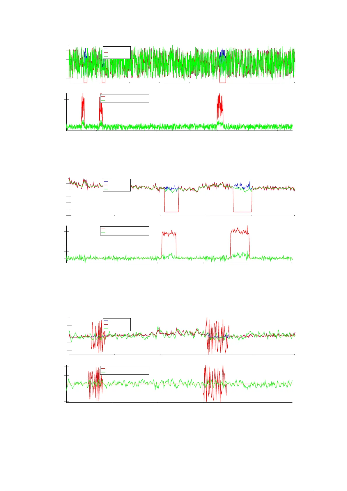
Stac k ed auto enco ders based mac hine learning for noise reduction and signal reconstruction in geoph ysical data Deb jani Bho wmick 1 † Deepak K. Gupta 2 † Saumen Maiti 3 Uma Shank ar 4 1 Cognitiv e Science & Artificial Intelligence, Tilburg Universit y , The Netherlands 2 Informatics Institute, Univ ersity of Amsterdam, The Netherlands 3 Dept. of Applied Geoph ysics, Indian Institute of T echnology (ISM) Dhanbad, India 4 Dept. of Geophysics, Banaras Hindu Universit y , V aranasi, India Abstract Auto encoders are neural netw ork formulations where the input and output of the netw ork are iden tical and the goal is to iden tify the hidden represen tation in the pro vided datasets. Generally , au- to encoders pro ject the data nonlinearly on to a low er dimensional hidden space, where the imp ortan t features get highligh ted and interpretation of the data becomes easier. Recent studies ha ve sho wn that even in the presence of noise in the input data, autoenco ders can be trained to reconstruct the noisefree comp onent of the data from the reduced-dimensional hidden space. In this pap er, we explore the application of autoenco ders within the scope of denoising geoph ysical datasets using a data-driv en methodology . The autoenco der formulation is discussed, and a stack ed v arian t of deep autoenco ders is prop osed. The prop osed metho d in volv es lo cally training the weigh ts first using basic auto encoders, eac h comprising a single hidden lay er. Using these initialized weigh ts as starting p oin ts in the optimization mo del, the full auto encoder netw ork is then trained in the second step. The applicability of denoising auto encoders has b een demonstrated on a basic mathematical example and several geophysical examples. F or all the cases, auto encoders are found to significantly reduce the noise in the input data. 1 In tro duction Mac hine learning has b een a trending topic in the past t wo decades, and it has widely b een used in v arious science and engineering disciplines for improv ed interpretation of big datasets. Creating a ma- c hine learning algorithm essentially refers to building a model that can output appro ximately correct information when fed with certain input data. These mo dels can b e thought of as black-boxes: input go es in and output comes out - although the mapping from input to output can b e fairly complex in itself. With the adv ent of p o werful computers, it has b ecome remark ably easy to train the computers to iden tify the hidden complex representations in pro vided datasets. F or an o verview of the applications of mac hine learning in v arious fields, see the recent review w orks presented in [58, 15, 26, 24, 25], among others. Among the v arious machine learning metho ds, neural netw orks in particular, ha ve receiv ed enormous atten tion. Here, we list some of the early works related to application of neural netw orks in v arious sectors. F or a detailed o verview, please see the citing references to these pap ers. In the finance sector, neural net works are used for bankruptcy prediction of banks/firms [50], future options hedging and pricing [20], credit ev aluation [23], in terest rate prediction [35], in ter-market analysis [49] and sto ck performance [5]. In human resources, the pro cesses of p ersonnel selection and w orkplace behavior prediction are automated using this tec hnique [40, 13]. In the information sector, neural netw orks ha ve widely b een used for authen tication or iden tification of computer users [43], recognition and classification of computer viruses [16], pictorial information retriev al [55], etc . Recently , neural net works hav e b een used to solve sev eral challenging problems in the field of medical imaging. F or example, with this p o werful tool, lung cancer can b e effectiv ely diagnosed and differentiated from lung benign diseases, normal con trol and gastroin testinal cancers [17]. There is an unending list of other applications where neural netw orks hav e pro ved to b e w orthy , and not all of these can be listed here. † During this research, D. Bhowmic k was affiliated with Indian Institute of T echnology , ISM Dhanbad, India and Coal India Limited, Ranc hi, India, and D. K. Gupta w as affiliated with Delft Univ ersity of T echnology , The Netherlands. 1 The discipline of geophysics is no exception and neural netw orks ha ve b een used on v arious geophys- ical problems, e.g. , in version of electromagnetic, magnetelluric and seismic data [39, 65, 46], w av eform recognition and first-break picking [34], trace editing [32], lithological classification [30], guide geoph ys- ical and geological modeling pro cess [42], creating ensem ble mo dels for the estimation of p etroph ysical parameters [8], etc . The ob jectiv e of most of the neural netw ork based form ulations is to mimic the in ternal represen ta- tion of the highly nonlinear mapping from input to output. It could either be a classification problem where the correct label needs to b e identified for a given input, or a regression problem where correct estimation of a resp onse is desired. An autoasso ciativ e net work (autoassociator) is an artificial neural net work form ulation which tries to learn the reconstruction of input using backpropagation. Thus, for an autoasso ciator, the input is same as the output and an approximation to the identit y mapping is obtained in a nonlinear setting. In the past, some researchers hav e used neural net works as autoasso- ciators with the aim of extracting sparse internal represen tations of the input data ( e.g. [3, 14, 12]). Ho wev er, the use of insufficient la yers restricted the generalization of these net works, therefore limiting their applicabilit y . Kramer [27] used three hidden lay ers comprising linear and nonlinear activ ations and show ed the applicability of their autoasso ciator for gross noise reduction in pro cess measuremen ts. Ho wev er, for cases where the features of a pro cess are related through a complex nonlinear function, the use of even three hidden la yers ma y not necessarily be sufficient for certain cases. Bengio [7] presented auto enc o der , a form of autoasso ciators in a deep net work framewor k, which allo wed learning more accurate internal representations of the input. Since ‘autoenco der’ is a more com- mon term in the recent literature, the rest of the paper uses it o v er ‘autoasso ciators’. Auto enco ders ha ve primarily b een used to reduce the dimensionalit y of large datasets. A pro jection to a lo w er dimensional space helps to iden tify sev eral hidden features and promotes improv ed in terpretation of the data. Vincen t et al. [61] used autoenco ders for denoising tasks b y c heaply generating input training data and corrupting it. This denoising procedure w as aimed at making autoenco ders more robust and allow ed reducing the dimension of data efficien tly even in the presence of noise. V alen tine and T ramp ert [59] presented the geoph ysical application of auto encoders for data reduction and qualit y assessmen t of wa veform data. The pap er presented a precise and clear o verview of the classical auto enco der theory , follow ed by its application on seismic wa veform data. Since then, auto encoders ha ve already been used for a few other problems e.g. analysis of top ographic features [60], identification of geochemical anomalies [64]. Amongst sev eral others, one of the biggest c hallenges in geophysics is the denoising of data. The problem of noise remov al from data is v ery common with v arious other disciplines, and has b een studied extensiv ely in the past. Some of these are based on lo cal smoothing to blur the noise e.g. nonlinear total v ariation based approac hes [48], anisotropic diffusion metho d [62], bilateral filtering [57], etc . Other category of denoising approaches in volv es learning on noise-free datasets and then exploitation of noisy datasets [63, 21, 47]. One such w ay is to learn using wa velets and then shrink age of the co efficien ts to remo ve the noise [37, 38]. W av elet based shrinking has b een used on v arious geophysical problems, e.g. seismic noise attenuation [6, 29]. In the context of denoising, limited researc h has b een done in the past to inv estigate the applicability of auto encoders. Recently , Burger et al. [10] used autoenco ders in a deep netw ork framework for denoising input images and the approach w as found to outp erform some and p erform equal to other state-of-art denoising metho ds. Sc huler et al. [53] presen ted a neural netw ork based non-blind image deconv olution approac h capable of sharp ening blurred images. The netw ork w as trained on large datasets comprising noisefree as w ell as noisy images, and it was found to w ork well for the task of denoising. Ojha and Garg [36] used auto encoders for denoising high-resolution m ultisp ectral images. It was sho wn in this pap er that after training the model on a large set of noisy and denoised images, results comparable to non-lo cal means algorithm are obtained in a significan tly lesser amount of time. Clearly , the works on denoising outlined abov e ha ve demonstrated the p otential of autoenco ders. In a recen t w ork, w e ha ve briefly sho wn that denoising autoenco ders work very well for geoph ysical problems [9], and it is of in terest to explore further in this direction. In this pap er, w e study in detail the application of auto enco ders for denoising geophysical data. This w ork revolv es around using autoenco ders to learn the representation of the signal, and separate the noise conten t. W e start with exploiting the p otential of shallo w auto enco ders for denoising purp ose. Based on the identified limitations of these net works, deep auto encoders with several differen t num b er of hidden lay ers are tested. T o further enhance the denoising c haracteristic of the auto encoders, a stack ed form ulation is presen ted, the application p oten tial of whic h is demonstrated on v arious numerical examples. Here, we discuss the outline for the rest of the paper. The theoretical details of autoenco ders are discussed in Section 2. This includes a brief description of the traditional autoenco ders (Section 2.1) 2 f θ ( x ) g θ 0 ( y ) x z y Figure 1: Schematic structure of a traditional neural net work. F or x ≈ z , the netw ork corresponds to an autoasso ciator/autoenco der. follo wed by its denoising v ariant (Section 2.2). The concept b ehind the stac king of auto encoders is discussed in Section 2.3. T o demonstrate the working of auto encoders for denoising tasks, a basic mathematical example is presen ted in Section 3. The applications on geophysical problems are discussed in Section 4 and the final discussions and conclusions are presented in Sections 5 and 6, resp ectiv ely . 2 Theory 2.1 Auto enco der Auto encoders aim at learning the in ternal represen tation of data, typically enco ding, and iden tify the imp ortan t hidden features [7]. In its simplest form, an autoenco der is v ery similar to a m ultilay er p erceptron (MLP), which consists of an input lay er, an output lay er, and one or more hidden lay ers. F or an ideal autoenco der, the input and output are same, which implies that the hidden units need to b e tuned such that an accurate nonlinear appro ximation to the iden tity function can be obtained. When neural net works are used, our interest is in learning an internal represen tation that relates the input to the output. Fig. 1 shows the schematic diagram of a neural netw ork, where x and z are the input and output vectors, respectively . The output vector z is obtained from x through a series of linear/nonlinear mappings denoted by f θ ( · ) and g θ 0 ( · ) functionals, resp ectiv ely . F or a deep net work, these mappings themselves could comprise several hidden lay ers. The v ector y in Fig. 1 corresp onds to a hidden lay er in the netw ork with reduced dimensionality . F or the netw ork sho wn in Fig. 1 to b e formulated as an autoenco der, x and z need to b e ideally the same. Generally , the dimensionalit y of the hidden la yers ( e.g. y ) is kept lo wer than that of the input and output, which allows auto enco ders to learn an appro ximate compressed representation of the input. As discussed in [61], a natural criterion that an y goo d representation should b e exp ected to meet is that a significan t amount of information ab out the input is retained. How ever, this condition alone is not sufficien t to yield a goo d representation. Using hidden la yers of same dimensionality or higher can lead to iden tity mapping, whic h is unlikely to lead to an y useful information. Although traditionally follo wed, it is not necessary to use hidden la yers of lo wer dimensions, rather, these can b e larger than the input. With the constrain t of reduced dimensionality in the hidden lay ers, autoenco ders can provide an alternativ e reduced-dimensional represen tation of the massive datasets, pro viding a no vel insigh t into the data. Adding sparsit y constraint allo ws using higher dimensionalities and it has b een observed that these can provide very useful feature representations ( e.g. [44]). An adv an tage of the sparse auto encoders is that they can handle v ariable-sized representations [61]. A simplified version of an auto enco der, where no nonlinear transformations are used and a squared-loss error function is emplo yed, is equiv alent to p erforming principal comp onen t analysis (PCA) [4]. How ever, this is generally not true for the traditional auto encoders where sigmoid-based nonlinearit y exists. A traditional autoasso ciator consists of tw o parts: an enc o der and a de c o der . Lo oking back at Fig. 1, let us assume that the sho wn neural net work corresponds to an autoenco der with one hidden la yer. Thus, y corresp onds to the hidden represen tation with reduced dimensionalit y . The mapping phase where the input x is transformed in to the hidden representation y is termed as an enco der. A decoder is the part of an auto encoder where the input is reconstructed back as z from its hidden representation y . In Fig. 1, the enco ding and decoding functions are denoted by f θ ( · ) and g θ 0 ( · ), resp ectively and these mappings are parametrized b y v ectors θ and θ 0 , resp ectively . Typically , the mapping functions comprise of affine 3 ˜ x = x + ∆x x y Enco der Deco der × × Figure 2: Sc hematic diagram of a denoising auto encoder showing the enco der and decoder segments. The netw ork comprises 3 hidden la yers of 7, 5 and 7 neurons, respectively . mapping follow ed b y certain nonlinearit y and can be expressed as: f θ ( x ) = S ( Wx + b ) , (1) g θ 0 ( y ) = S ( W 0 y + b 0 ) , (2) where, θ = { W , b } and θ 0 = { W 0 , b 0 } are parameter sets with W and W 0 denoting the w eight matrices and b and b 0 represen ting the bias v ectors, resp ectiv ely . Typically the nonlinear mapping S ( · ) is achiev ed using sigmoid or radial basis functions. The goal of the auto encoder presented in Fig. 1 is to minimize the reconstruction loss b et ween x and z . As error (loss) function, typically squared-error function or cross-entrop y loss are used dep ending on the type of problem. The auto encoder presen ted in Fig. 1 consists of a single hidden lay er. How ev er, for auto enco ders of higher complexit y , several hidden lay ers can b e used. Accordingly , the enco der and deco der will then comprise of a series of mappings in each. F or more details related to auto enco ders, see [61]. 2.2 Denoising auto enco der An y mo del can be considered as a goo d denoiser, if it can output clean signal from a noisy input. The first and foremost thing needed to build a denoising auto enco der is to iden tify a mapping from the noisy domain to the noisefree domain. The complexit y of this mapping dep ends on sev eral factors ( e.g. level of noise), and cannot be expressed using a simple form ula. How ever, if there exist a large num b er of data samples, auto encoders can be used to determine the fitting empirical mo del [10]. As outlined in [61], the concept of denoising auto encoders is based on the follo wing ideas: • The higher level representation of the input data ( i.e. primary signal) is generally assumed to b e more stable and robust to addition of noise. • Denoising approac h should b e able to capture the features associated with the primary signal in the inner hidden lay ers of the netw ork. T ypically , it is assumed that our primary signal has a certain well-defined representation, while noise may ha ve it or may not. F or non-coherent noise, the denoiser needs to b e trained to filter our the comp onen ts of input data which do not comprise any w ell-defined pattern. F or coherent noise, the denoiser has to b e trained such that it preserv es the represen tation of the signal, but filters out the noise component. Remo ving coheren t noise can b e a challenging problem, esp ecially when the signal-to-noise ratio is quite lo w. Fig. 2 sho ws the schematic netw ork representation for a basic denoising auto encoder. The auto en- co der comprises three hidden la yers of 7, 5 and 7 neurons resp ectiv ely , and the input consists of 9 features. Compared to the input,the dimensionalit y of the innermost representation is 44% low er, whic h means 4 ˜ x x ˆ y 1 ˆ y 1 ˆ y 1 ˆ y 2 ˆ y 2 ˆ y 2 ˆ y 3 ˆ y 2 ˆ y 2 ˆ y n + 1 2 ˆ y n − 1 2 ˆ y n − 1 2 g θ 0 1 f θ 1 g θ 0 2 f θ 2 g θ 0 3 f θ 3 g θ 0 n − 1 2 f θ n − 1 2 ˜ x x y 1 y n y 2 y n − 1 y n +1 2 y n +3 2 y n − 1 2 Step 1 : Recursively training the shallo w auto enco ders for the pre-initialization of weigh ts Step 2 : T raining the full netw ork with pre-initialized weigh ts obtained from Step 1 × × Figure 3: Schematic diagram of a stack ed denoising auto enco der showing the t wo steps in v olved in the denoising pro cess. The en tire deep net work is assumed to comprise n hidden la yers. During Step 1, the w eights are trained for one hidden la yer at a time, in a recursiv e manner. Finally , during Step 2, the en tire netw ork is trained at once using the pre-initialized weigh ts obtained from Step 1. that a compressed representation of the input will b e enco ded, and there can p ossibly b e a loss of certain features. The goal is to train this net work to construct clean output x from the corrupted v ersion ˜ x . Through a series of tw o pro jections (let us assume f θ ( ˜ x )), the noisy signal ˜ x is mapp ed on to a reduced dimensional space, and the result is y . The functional f θ ( · ) here refers to the encoder part of the auto enco der. Ideally , from the hidden represen tation y , the noisefree signal x needs to be constructed, and this process is referred to as decoding ( x = g θ 0 ( y )). During the optimization pro cess, this is ac hieved b y training the set of parameters θ and θ 0 and obtaining output z , such that the reconstruction error  ( x , z ) is minimized. Vincen t et al. [61] ha ve pro vided a nice geometrical in terpretation for denoising autoenco ders. This in terpretation is based on the so-called manifold assumption ([11]), according to which natural high- dimensional data concentrates close to a non-linear lo w-dimensional manifold. Generally , the noisefree data can be understo o d as a combination of sev eral principal components, and using a neural net work arc hitecture, it is possible to obtain these components. Noise is generally found to b e shifted a w ay from these manifolds, and in the pro cess of minimizing the loss, the optimization pro cess tends to not include the noise comp onen t in the reduced dimensionalit y . 2.3 Stac k ed auto enco ders T raining the autoenco der to remo ve noise from a giv en dataset can be highly nonlinear and is not an easy problem to solv e. Learning such complex representations requires deep m ulti-lay ered neural net works. The standard approach, comprising random initialization of w eigh ts and using gradient descent based bac kpropagation, is kno wn to pro duce p oor solutions for 3 or more hidden lay ers. In [28], this asp ect has b een studied in detail, and it has b een observed that if efficien t algorithms are used, deep architectures p erform better than shallo w ones. In this pap er, a stack ed formulation for auto encoders is prop osed, where m ultiple cycles of simple auto encoders are trained in a zoom-in fashion, follow ed b y training the whole net work at once. Fig. 3 sho ws the sc hematic diagram explaining the t wo steps of stac ked denoising auto encoder. It is assumed that the deep netw ork architecture of the auto encoder comprises n hidden lay ers. The details related to the tw o steps follo w b elo w. 5 2.3.1 Recursiv e pre-training of weigh ts and biases In this step, the w eights and biases of the net w ork are pretrained using simple autoenco ders comprising 1 hidden la y er each. F or n hidden la yers in the deep autoenco der net work, a total of ( n + 1) / 2 autoenco ders need to b e formulated due to symmetry in the netw ork architecture. Here, it is assumed that n is an o dd n umber as sho wn in Fig. 3. The w eights corresponding to the hidden la y ers are determined, starting with the outermost hidden lay ers and moving to wards the innermost represen tation in a recursiv e manner. Let ˜ x and x denote the noisy signal and its uncorrupted version, respectively . Let f θ 1 ( · ) and g θ 0 1 ( · ) denote the pro jection of x onto the first hidden lay er space (where the represen tation is denoted by ˆ y 1 ) and pro jection from the hidden lay er to the output space, resp ectiv ely . This implies that ˆ y 1 = f θ 1 ( ˜ x ) and x = g θ 0 1 ( ˆ y 1 ). Note here that after the autoenco der has been trained, there will still b e an approximation error, and g θ 0 ( ˆ y 1 ) may not necessarily b e equal to x . Once the parametrization vectors θ 1 and θ 0 1 ha ve b een trained, the next inner representation needs to b e optimized. F or training the next level representation, an auto encoder comprising a 3-la yer neural netw ork is form ulated. The input and output v ectors for this autoenco der are set to ˆ y 1 eac h. The resp ectiv e mappings on to the hidden space and the output space are denoted by f θ 2 ( · ) and g θ 0 2 ( · ) functionals, resp ectiv ely . The parameter v ectors θ 2 and θ 0 2 are optimized, and ˆ y 3 is computed. This whole pro cess of formulating an auto encoder and computing level hidden lev el representation is repeated n +1 2 times as sho wn in Fig. 3 and ˆ y 1 , ˆ y 2 , . . . , ˆ y n +1 2 are obtained. A t the same time, parameter vectors θ 1 , θ 2 , . . . , θ n +1 2 and θ 0 n +1 2 , θ 0 n − 1 2 , . . . , θ 0 1 ha ve been optimized to certain v alues. 2.4 T raining the full net w ork Once the parametrization vectors hav e been initialized, Step 2 inv olves further training the en tire deep net work at once. The deep net work arc hitecture has been shown in Fig. 3. The input and output vectors for this netw ork are set to ˜ x and x , respectively and the parameters for the lay ers from left to righ t are set to θ 1 , θ 2 , . . . , θ n +1 2 , θ 0 n +1 2 , θ 0 n − 1 2 , . . . , θ 0 1 . Accordingly , the mapping functionals from left to right of the net work are defined to be f θ 1 ( · ), f θ 2 ( · ), . . . , f θ n +1 2 ( · ), g θ 0 n +1 2 ( · ), g θ 0 n − 1 2 ( · ), . . . , g θ 0 1 ( · ), respectively . Once the whole netw ork has been set up and the parameters hav e b een initialized with the v alues computed in Step 1, optimization is p erformed and the ne w representations for the n hidden lay ers of the deep net work are obtained. These are denoted by y 1 , y 2 , · · · , y n . 3 A basic mathematical example T o pro vide a b etter understanding of ho w an autoenco der works, here we presen t a basic mathematical example. Since the goal of this pap er is t ypically to demonstrate the use of auto encoders for noise reduction and data reconstruction and excludes its usage as merely a dimensionalit y reduction tool, w e restrict ourselves to denoising auto encoders. F or readers interested in the application of autoenco ders for dimensionality reduction in geoph ysics, we advise looking at the w ork of [59]. T o start with, a simple mathematical problem of t wo parameters ( z and θ ) is chosen and a pro cess mo del of the follo wing form is used [18], x = tz sin θ + t 2 z cos θ , t = 0 . 05 : 0 . 05 : 1 , z ∈ [0 . 5 , 4 . 0] , θ ∈ [0 . 3 , 1 . 3] in radians. , (3) where, t and x are the input and output fields, resp ectiv ely , and z and θ are the mo del parameters. F or t , a range of 0.05 to 1 is c hosen with a sampling in terv al of 0.05. The input field t = { 0 . 05 , 0 . 1 , . . . , 1 . 0 } is then used to generate the output signal x = { x 1 , x 2 , . . . , x n } , where n denotes the num b er of sampling p oin ts. Once x is obtained, it is assumed that the pro cess model is not kno wn anymore. Next, an auto encoder is trained to learn the in ternal represen tation of x suc h that for any noisy v ariant ˜ x , the noise-free signal can b e reco vered. Learning the representation here refers to approximating the process mo del through a neural net work and rejecting the component of the input whic h does not fit w ell with the mo del. An autoenco der comprising 2 hidden lay ers is formulated. The num b er of neurons in each hidden la yers is k ept to b e equal to n . Note that c ho osing the n umber of neurons equal to the num b er of input units here does not lead to a plain identit y function due to the large noise added in some of the signals. T able 3 states the neural net work parameters used for this auto encoder. Nonlinear (sigmo dial) activ ation 6 T able 1: Parameters for the simple denoising autoasso ciativ e neural net work used in Section 3. P arameter V alue TRAINING PHASE No. of samples 20000 Noisy samples 10000 Noise type random noise (upto 25%) T raining samples 80% V alidation samples 20% No. of hidden lay ers 2 Hidden units { 20, 20 } Activ ation functions { sigmoid, sigmoid, linear } TEST PHASE T est samples 100 noise b et w een 10% and 25 % 20 40 60 80 100 0 20 40 60 80 test sample index η % (a) Noise reduction η for the test data 0 . 2 0 . 4 0 . 6 0 . 8 1 0 0 . 2 0 . 4 0 . 6 0 . 8 1 1 . 2 t x noise-free noisy AE corrected (b) T est sample 20 0 . 2 0 . 4 0 . 6 0 . 8 1 0 0 . 2 0 . 4 0 . 6 0 . 8 1 1 . 2 t x noise-free noisy AE corrected (c) T est sample 70 Figure 4: (a) Relativ e noise reduction η for the 100 noisy test samples, (b) noise-free, noisy and autoen- co der (AE) corrected data for sample index 20 and (c) for sample index 70. A denoising auto enco der comprising 2 hidden lay ers with 20 neurons in eac h is used. functions are used for pro jection from the input la yer to hidden la y er 1 and hidden la yer 1 to hidden lay er 2. F or obtaining the output z , linear activ ations are used. The error (loss) function J ( · , · ) is defined as J ( x , z ) = N s X i =1 ( x − z ) | ( x − z ) N s , (4) where, N s refers to the n umber of samples,and x and z refer to the noise-free and recov ered samples, resp ectiv ely . A set of 20000 samples is generated using the process mo del stated in Eq. 3, and is further divided in to 80% and 20% for training and v alidation samples, resp ectively . Random noise of upto 25% is added to the data p oin ts of 10000 samples and the other 10000 samples are k ept noise-free. F or 50% of the noisy-samples, the magnitude of added noise scales based on the lo cal v alue at the resp ectiv e p oin t of the sample. F or the remaining 50%, it scales with the mean of all the data points of the sample. F or optimization purp ose, the traditional gradien t descen t algorithm is used. Due to the simplicit y of the problem, no regularization is needed, and the conv ergence of the optimization problem is found to be v ery fast. T o test the accuracy of the learnt represen tation Φ , 100 test samples are generated, and noise, chosen randomly betw een the levels of 10% and 25%, is added to each of these samples. Next, these data samples ˜ x are passed through the learnt represen tation to reduce the noise and obtain the output z = Φ ( ˜ x ). The efficiency η of the learnt represen tation Φ for any noisy signal ˜ x is given b y η = 100 × ( z − x ) | ( z − x ) ( ˜ x − x ) | ( ˜ x − x ) % . (5) Fig. 4a sho ws the η v alues for 100 noisy samples measured using Eq. 5. F or these samples, the mean v alue of η is found to b e η = 90 . 27%, which means that the learnt auto encoder Φ can reduce the noise 7 r − r 0 r 0 P ( r ) θ d Figure 5: Schematic diagram of a buried vertical cylinder, also showing some of the parameters that c haracterize the 1D SP anomaly caused due to it. b y approximately 90%. This is a significant improv ement and clearly demonstrates the applicability of auto encoders for denoising purp ose. Figs. 4b and 4c sho w tw o data samples, their noisy versions as w ell as the auto enco der corrected signals. These data samples ha v e b een pick ed randomly from the set of 100 samples for demonstration purp ose . F rom the results, it is clear that the autoenco der has learn t to iden tify the signal pattern within the data, and reject any random noise. 4 Applications 4.1 Self-p oten tial problem In a self-p oten tial (SP) surv ey , the naturally o ccurring potential differences generated b y electro c hemical, electrokinetic and thermoelectric sources are measured. This approach has been used in a wide range of applications: in exploration mainly for sulphides and graphite [56], ground water inv estigations [52], detection of ca vities [22] and geothermal exploration [66]. F or some cases, SP anomaly can b e mo deled using simple geometries, e.g. sphere, cylinder and inclined sheet [51]. F rom the obtained field data, the set of parameters defining the buried source can be determined using v arious metho ds suc h as curve matc hing [33], gradien t-based metho ds [2], global optimization [19], etc. The SP data acquired in the field can also comprise noise from several sources, and without any post- pro cessing, it is possible that the inv erted set of parameters defining the buried source do not comply w ell with the actual properties. With the gradient-based methods, there exist high chances of getting stuc k in a local optimum. The global optimization methods as well hav e b een found to be sensitive to the lev el of noise in the data ( e.g. [51, 19]). T o circum ven t this problem, w e use auto encoders for reducing the noise conten t in the acquired data. In the con text of SP anomaly inv ersion, the application of auto encoders is demonstrated on data obtained for a 1D problem. A v ertical cylinder buried in the subsurface, as shown in Fig. 5, is considered. The forward mo del for the SP anomaly at a p oin t P ( r ) is computed as V ( r ) = K ( r − r 0 ) cos θ + d sin θ (( r − r 0 ) 2 + d 2 ) q , (6) where, d , θ , K and q denote depth, p olarization angle, current dip ole moment and shape factor, re- sp ectiv ely , and r 0 refers to the origin of the anomaly . These five v ariables are the parameters obtained generally by inv erting the SP data. Note that in this w ork, we are not dev eloping another efficient in version approac h. Rather, with the forw ard mo del kno wn, our goal is to train the neural net work to b e able to iden tify the component of data that complies with it, and reject the other parts. T o start with, w e define ranges for the parameters stated in Eq. 6, and these are shown in T able 2. Com binations of parameters’ v alues are randomly chosen from these ranges to generate data samples for training the neural netw ork. The v alue of r is v aried from -20.0 m to 20.0 m with a spacing of 2.5 m. As stated in T able 3, a total of 60000 samples are used, out of whic h 40000 samples are corrupted with random noise. The en tire dataset is divided into training and test sets in the ratio of 4:1. All the lay ers 8 T able 2: Range of v alues for the parameters characterizing the forward mo del for 1D SP anomaly caused due to the burial of a v ertical cylinder ([51]). P arameter Min Max depth d (m) 1 8 p olarization angle θ (degrees) 25 75 electric dip ole momen t K (mV) -1000 1000 shap e factor q 0.5 1.5 origin of the anomaly r 0 (m) -5 5 T able 3: Netw ork parameters for the v arious (stac ked) denoising autoenco ders used for reduction of noise in self-p oten tial data. P arameter V alue TRAINING PHASE No. of samples 60000 Noisy samples 40000 Noise type uniform random noise Noisy units p er sample 50% T raining samples 80% V alidation samples 20% Activ ations all sigmoid and last as linear TEST PHASE T est samples 1000 Noisy units p er sample 50% Noise random (upto 50) % comprise sigmoid activ ations, except the last one which has only a linear activ ation. The loss (error) at ev ery step of training is computed in a similar fashion as stated in Eq 4. F urther, to get the quantitativ e estimate of the noise reductions, w e use the function η stated in Eq. 5. Sev eral different auto encoder configurations are tested to understand ho w complexity and comp osition of the neural netw orks affect the performance of auto enco ders. T able 4 lists the num b er of neurons in eac h lay er for the v arious auto encoders used. It is observ ed that with shallow auto enco ders (SA), which comprise up to tw o hidden la yers, the reduction in noise is less than 60%. F or the net work with one hidden la yer comprising only 4 neurons, noise reduction level is merely around 17%. This happ ens b ecause such a compressed internal representation migh t not b e enough to fully capture the signal pattern. Increasing the num b er of hidden lay ers to 12 already pushes the efficiency η of the auto encoder beyond 50%. The use of deep autoenco ders (DE) with 3 or more lay ers has b een observed to further impro ve the p erformance. With 3-5 hidden la yers, η reac hes close to 65% (T able 4). An in teresting observ ation is that with increasing num b er of hidden lay ers, the v alue of η reduces. This is because as the netw ork grows, training it b ecomes more difficult due to the increased num b er of v ariables and v anishing gradients. Clearly , with these b ottlenec ks, the conv entional deep net works are not the right solution to obtain v ery efficien t auto enco ders for the SP problem. T o circum v ent the issue related to training the deep net works in a standard manner, w e explore the application of stack ed auto enco ders for denoising SP data. Several neural net work configurations are tested using the t w o step approach describ ed in Fig. 3. In the first step, the w eights corresp onding to ev ery hidden lay er are trained using basic auto enco ders with only one hidden lay er each. Once the w eights ha ve been initialized, a full-fledged deep neural net work is trained to reach the final solution. Stack ed auto encoders hav e b een found to push η beyond 70%. This can be impro ved further by regularizing the weigh ts and av oiding o ver-fitting. With 5 hidden la yers, the stack ed autoenco der could achiev e efficiencies close to 78%. Fig. 6 sho ws three data samples chosen randomly out of 1000 data samples in the test set. A stac ked deep net work with 5 hidden lay ers is used. It is observed that for the three cases, auto enco der could significan tly reduce noise in the data. Ho wev er, in Fig. 6c, certain amount of bias can be seen in some parts of the result obtained using auto encoder. Although the emplo y ed auto enco der could smo othen the data in that region, the asso ciated v alues deviate significan tly from the actual v alues. A reason could b e that the training set did not comprise samples resem bling this data, and the mo del w as not sufficiently trained for it. Clearly , a remedy would b e to further train the mo del in a feedback lo op based on the 9 T able 4: Information related to runs of denoising SP data using sev eral autoenco der configurations. Here, SA, D A, SD A and SDA-R refer to shallow auto enco ders, deep auto encoders, stack ed deep autoenco ders and stac ked deep autoenco ders with randomness, respectively . Also λ defines the exten t of regularization η denotes p ercen tage reduction in noise. Hidden no des Net work-t yp e λ η (in %) { 4 } SA 0.0 17.6 { 12 } SA 0.0 54.7 { 25 } SA 0.0 55.4 { 12, 12 } D A 0.0 58.4 { 20 25, 20 } D A 0.0 65.4 { 17, 20 25, 20 } D A 0.0 64.1 { 20 25, 30, 25, 20 } D A 0.0 63.7 { 20 25, 20 } SD A { 0.0, 0.0; 0.0 } 61.8 { 20 25, 20 } SD A { 0.05, 0.05; 0.0 } 70.9 { 20, 25, 30, 25, 20 } SD A { 0.05, 0.05; 0.05; 0.0 } 73.0 { 20, 25, 30, 25, 20 } SD A-R { 0.05, 0.05; 0.05; 0.0 } 78.5 { 25 20, 17, 20, 25 } SDA { 0.0, 0.0; 0.0; 0.0 } 72.1 { 35 25, 17, 25, 35 } SDA { 0.05, 0.05; 0.05; 0.0 } 77.2 { 35 25, 17, 25, 35 } SD A-R { 0.0, 0.0; 0.0; 0.0 } 80.6 { 35 25, 17, 25, 35 } SD A-R { 0.05, 0.05; 0.05; 0.0 } 81.3 − 20 − 10 0 10 20 0 2 4 6 8 10 r (in m) V ( r ) (in volts) noise-free noisy AE corrected (a) T est sample 27 − 20 − 10 0 10 20 0 50 100 150 r (in m) V ( r ) (in volts) noise-free noisy AE corrected (b) T est sample 73 − 20 − 10 0 10 20 − 600 − 400 − 200 0 200 r (in m) V ( r ) (in volts) noise-free noisy AE corrected (c) T est sample 282 Figure 6: Noise-free, noisy and autoenco der (AE) corrected data for samples with index 27, 73 and 282. These samples ha ve b een c hosen randomly out of the 1000 test samples. The noisy signal consists of upto 50% random noise in 50% of the p oin ts for each sample. A stack ed deep netw ork with the hidden structure of { 25, 20, 17, 20, 25 } is used. fitting obtained for such examples. W e also observ ed that for stack ed auto enco ders, perturbing the w eights obtained in step 1 improv es the conv ergence of ste p 2. Randomly 10% of the w eights corresp onding to each hidden la yer are sampled and perturb ed b y up to 5%. With this configuration, η v alue of 80.6% is obtained. This approach when com bined with regularization can remo ve more than 81% of the noise from SP data. With this level of impro vemen t in the data, it can b e claimed that stack ed auto encoders could b e a p oten tial denoising to ol for suc h problems. 4.2 Seismic data In this section, the applicabilit y of auto encoders is explored for the remov al of random noise from seismic data. As stated earlier, the application of autoenco ders on seismic w av eform data has been demonstrated in the past by [59], ho wev er, only in the context of dimensionality reduction. Here, our goal is to remo ve noise from seismic data. F or simplification purpose , w e do not discuss the headers associated with the data, rather w e treat the seismic data only as a tw o-dimensional matrix of amplitude v alues. Also, in this pap er, our scop e is restricted to non-coherent noise, and cases of coherent noise are not considered. Fig. 7 shows the seismic section that has been used in this study to generate training and test samples for the auto encoder net w ork. 10 time (in sec) T race n umber Figure 7: An example seismic section considered for generating the training and test samples for this study . n m ˜ n ˜ m ˜ s = 1 test image Figure 8: Sc hematic diagram demonstrating the extraction of small image slices from a test image of size m × n . F or the se ismic example case, m and n w ould denote time samples and num b er of traces, resp ectiv ely . The image slices are c hosen to b e of size ˜ m × ˜ n and stride ˜ s = 1. T able 5: Netw ork parameters for the v arious (stac ked) denoising autoenco ders used for reduction of noise in self-p oten tial data. P arameter V alue TRAINING PHASE Sample size 9 × 42 No. of samples 1.1 million Noisy samples 0.75 million Noise type monofrequency sinusoidal noise Noise frequency b et w een 100 and 220 Hz Noisy traces p er sample 1 T raining samples 95% V alidation samples 5% Activ ations all sigmoid and last as linear D A netw ork { 300, 400, 300 } SD A netw ork { 300, 400, 500, 400, 300 } Max. ep ochs 50000 TEST PHASE T est image size 99 × 42 Num b er of noisy traces 7 Noise type monofrequency sinusoidal noise Noise frequency b et w een 100 and 220 Hz windo w size 9 × 42 stride 1 11 10 20 30 40 10 20 30 40 50 60 70 80 90 (a) noise-free data 10 20 30 40 10 20 30 40 50 60 70 80 90 (b) noisy data 10 20 30 40 10 20 30 40 50 60 70 80 90 (c) corrected data obtained using a traditional deep auto encoder 10 20 30 40 10 20 30 40 50 60 70 80 90 (d) corrected data obtained using a stack ed deep auto enco der Figure 9: Denoising of corrupted seismic data using a traditional deep auto encoder and a stac ked deep auto encoder. F or the noisy data, some traces c hosen randomly , hav e b een corrupted b y replacing them with monofrequency sinusoidal traces in a frequency range of 100 to 220 Hz. 12 T able 6: Range of v alues for the three prop erty logs used to generate training dataset. Data source Porosit y (%) Clay fraction (%) Hydrate saturation (%) Syn thetic 1 30 - 60 50 - 80 0 - 20 K G basin (NGHP-01-05) 0 - 90 85 - 95 0 - 30 Mt. Elb ert-01, Alask a North Slop e 40 (approx.) 0 - 40 0 - 60 F or the purp ose of training the auto encoder, a total of 1.1 million small seismic samples are used. Details related to the training and test datasets are presen ted in T able 5. F rom the seismic section sho wn in Fig. 7, around 0.38 million smaller sample images are randomly chosen. Eac h sample image con tains 42 × 9 data p oin ts, 9 b eing the num b er of traces and 42 denoting the num b er of data points along the time axis for ev ery trace. These images are assumed to be the clean versions of data. F urther, eac h uncorrupted image is used to generate t wo noisy samples. A trace is randomly chosen from the clean image, and it is replaced b y a monofrequency trace with frequency in the range 100-220 Hz. The amplitude of the noisy trace is randomly c hosen b et ween 0 . 5 A max and A max , where A max refers to the maxim um amplitude observed in the seismic section. In this wa y , a total of around 1.1 million seismic samples are obtained. The en tire dataset is divided in to training and v alidation sets in the ratio 95:5. T o train the auto en- co der, first we start with 3 hidden lay ers comprising 300, 400 and 300 neurons, resp ectiv ely . All the activ ations are set to sigmoid, except the last one where linear activ ations are emplo yed. The w eigh ts are initialized randomly and the en tire netw ork is trained for up to 50000 ep o c hs. The trained mo del is then tested on a seismic image comprising 99 traces with 42 data p oin ts in each. Fig. 9a shows the clean image used for ge nerating test data. T able 5 lists complete details associated with testing the mo del. The noisy test data is generated by corrupting 7 traces in the noisefree test image as shown in Fig. 9b. The noisy traces corresp ond to monofrequency sinusoidal signals with frequency randomly chosen from the range 100-220 Hz. T o feed the test image to the trained mo del, compatible image slices need to be c hosen. These image slices are chosen using a windo w op erator, as shown in Fig. 8. This window is slid along the ro w and column directions of the image using a certain stride ˜ s . Here, ˜ s refers to the jump made b y the window p er step. F or a test image size of m × n , a window size of ˜ m × ˜ n and stride ˜ s = 1, a total of m − ˜ m +1 ˜ s × n − ˜ n +1 ˜ s image slices are fed to the trained mo del as shown in Fig. 8. Thus, the test seismic image used in this study is represented using 91 image slices. The output of the trained mo del is then summed up using a w eighted approach to obtain the output test image of the seismic section. The image slices are prop erly aligned and stack ed using w eights prop ortional to the n umber of times a data p oin t has been mapp ed in to an image slice. Fig. 9c sho ws the denoised v ersion of the noisy seismic image obtained using the auto encoder with 3 hidden la yers. It is seen that the chosen auto encoder netw ork could significan tly remo ve random noise from the data. Ho wev er, the auto enco der regularizes the seismic image due to which resolution of the image is lost to a certain exten t. Clearly , this is not desired, since the reduced resolution will lose information related to thin b eds as w ell as other fine features presen t in the seismic section. F urther, to test whether the random noise in seismic data can b e reduced without compromising to o m uch with the resolution of data, the potential of stac ked auto encoder net work is explored. A net work comprising 5 hidden la yers with 300, 400, 500, 400 and 300 neurons, respectively , is employ ed. In the first step of auto encoding, the w eights are initialized using sev eral traditional autoenco ders comprising single hidden la yer each. During the second step, the whole netw ork is trained using the pre-initialized w eights. The trained autoenco der is then used to denoise the test data. In the hidden la yer comprising 500 neurons, an additional sparsit y constrain t is added which ensures that not all the neurons of this la yer are activ ated at the same time. Fig. 9d sho ws the denoised seismic image obtained from the trained stac ked auto enco der. The random noise has b een significantly suppressed. Compared to Fig. 9c, it can also be seen that the resolution of the output image has significan tly increased. How ever, with this auto encoder configuration as w ell, the resolution of output seismic data is compromised to a certain extent. Nev ertheless, the stac ked auto encoder configuration shows p oten tial in suppressing noise in seismic data, and a future direction of research would be to design netw orks of even higher complexity that can pro duce b etter results. 13 f (1) φ (1) f (2) φ (1) f (3) φ (1) · · · · · · f ( n ) φ (1) f (1) φ (2) f (2) φ (2) . . . f (1) i − 1 f (2) i − 1 f (1) i f (2) i f (1) i +1 . . . f (2) i +1 f (1) ¯ φ (2) f (2) ¯ φ (2) f (1) ¯ φ (1) f (2) ¯ φ (1) f (3) ¯ φ (1) · · · f ( n ) ¯ φ (1) ¯ φ ( k ) = 2 i + m +1 2 − k φ ( k ) = 2 i − m − 1 2 + k Figure 10: Schematic diagram of an m × n image slice provided as a training sample to the denoising auto encoder. Here, the sup erscripts 1, 2, 3, . . . , n denote the features used for training. F or the w ell data denoising problem considered in this pap er, the features are p orosit y , saturation, p-wa ve v elo cit y and clay conten t. T o denoise the i th data p oin t in the well logs, the image slice includes information of m − 1 2 p oin ts ab o ve as w ell as b elo w this data point in the w ell logs. 4.3 W ell log data W ell logging is the practice of obtaining detailed information related to the geological formations in an area through sensors deplo yed in a borehole. This approac h has widely b een used to searc h for oil and gas, ground water, minerals as well as geotechnical studies. Sev eral differen t properties such as porosity , densit y , velocity , water saturation, etc. can b e estimated using well log data. Often for a certain geology , empirical linear/nonlinear relationships are established b et ween tw o or more suc h properties, and this is further used as a template to calculate one prop ert y if the other is kno wn. A detailed discussion on some such templates can be found in [31] and references therein. Amongst a set of logs acquired in a b orehole, it is p ossible that information in some parts of one log is either corrupted or missing. In case the data is missing, it can be calculated from other logs using appropriate empirical relationships. Here, the challenge is to identify the correct empirical relationship, since it dep ends very m uch on the lo cal geology . F or cases where one of the logs con tains some random noise, it might not be easy to iden tify it. In this paper, we explore the application of denoising auto encoders to solve the tw o issues outlined ab o v e. F or the first case, w e look at a suite of logs where parts of the data has b een corrupted. Next, w e train an auto encoder and use it to correct the data contained within this suite. In another test, parts of one of the logs are muted, and we let the trained auto encoder predict information in those parts. F or study purp ose, we use well log data from tw o gas h ydrate sites: NGHP-01-05 site in the Krishna-Go da v ari (K G) basin of India [54] and Mt. Elb ert (ME) site in the Alask a North Slop e region [45]. F or the t w o sites, the a v ailable logs are p orosit y ( φ ), shale volume ( V sh ) and p -wa ve velocity ( V p ). Using these logs, gas hydrate saturation v alues ( S h ) are calculated using the velocity-porosity transform prop osed in [41]. It comprises 3 relations b et ween v elo cit y and p orosit y , which are as follo ws. 0 ≤ φ < 0 . 37 , V p 1 = (1 − φ ) 2 V ma + φV f , (7) φ > 0 . 47 , 1 ρV 2 p 2 = φ ρ f V 2 f + 1 − φ ρ ma V 2 ma , (8) 0 . 37 ≤ φ ≤ 0 . 47 , 1 V p = φ − 0 . 37 0 . 1 V p 2 + 0 . 47 − φ 0 . 1 V p 1 , (9) where, V ma and V f denote matrix and fluid v elo cities, respectively . The data from the t wo sites has con trasting lithological comp osition, the K G basin sedimen t being shaly with around 80-90% cla y con tent in the ro c k matrix, and the ME data having lo w clay conten t and lo w p orosit y v alues. Due to this contrast, a single mo del that can fit these lithologies w ould hav e to be very nonlinear. 14 The goal of the denoising auto encoder for this case would b e to receiv e a suite of logs (4 logs for the examples ab o ve), and identify the parts of the data in the logs whic h do not satisfy the mo del of [41]. One reason could b e that one of the 4 logs for those parts of the data is corrupted with noise. Alternativ ely , it is p ossible that certain parts of the logs are missing, due to whic h the c heck cannot b e done. T o train the denoising autoenco der, a large set of training examples needs to be generated. Prior information related to the p ossible range of v alues for φ , S h , V p and V sh needs to be known. T able 6 lists the ranges for φ , S h and V sh that ha ve been used to generate the training set for this example. These ranges corresp ond to the range of v alues observed in KG basin and the ME site. In addition, a range of syn thetic data v alues has also b een added to make the auto encoder more robust and generalized. F rom these ranges, random v alues of φ , S h and V Sh are chosen and the corresponding v alue of V p is calculated using the model prop osed in [41]. The log prop erties are shifted using their resp ective means and normalized using their maximum and minimum v alues. The training samples need to b e fed to the autoenco der netw ork in the form of image slices of size m × n as sho wn in Fig. 10. Here, n denotes the num b er of prop ert y logs av ailable (equal to 4 for the example considered here). F or the i th data p oin t to be corrected, information from a total of m con tinuous data p oints needs to be considered, which includes m − 1 2 data p oin ts from ab o ve as well as b elo w the i th p oin t. In general, well log properties do not v ary muc h b et ween con tin uous data points. Although we include this fact in to our training data, we still allow the prop erties to v ary by up to 20% b et w een adjacent data p oin ts. In this manner, a total of 0.1 million clean images are generated. The auto encoder needs corrupted images as well for training. F or every clean image, 7 noisy images are generated. T o generate a noisy image, one of the 4 logs is randomly chosen, and b et ween 10% to 40% data p oin ts of this log prop ert y are mo dified. Either up to 10% random noise is added, or the data at these points is muted. The muted data p oints are set to -0.1 to differen tiate them from the rest of the data. Since there are 4 logs, n = 4. Tw o differen t auto enco der mo dels are trained with different v alues of m (3 and 70). The low v alue 3 is used to understand the lo cal c haracteristics of the data, and with 70, the goal is to understand the c haracteristics on a larger scale so that the noisy or m uted parts of the data can b e differen tiated from the noisefree parts. W e denote these m odels by Φ 3 and Φ 70 . The trained auto encoder is then tested on the test set. The real datasets from KG basin and ME site are used for this purp ose. Parts of the S h log from ME site and φ log from the K G basin site are m uted as shown in Figs. 11 and 12. Also, random noise is added in parts of the V p log of K G basin site as shown in Fig. 13. The ob jective of the trained auto encoders is to predict the correct information in these parts. F or quan titativ e impression of the added noise, the noisefree data is also sho wn in Figs. 11, 12 and 13. F rom the test dataset, several test image slices are generated as sho wn in Fig. 10. The concept of a sliding windo w, as discussed in Fig 8, is used with a stride of 1. Next, the tw o trained auto encoders Φ 3 and Φ 70 are applied on the input test data. The results obtained from the tw o trained auto enco ders are then summed up using w eigh ts 0.7 and 0.3, resp ectiv ely . These w eights ha ve b een obtained empirically using a trial and error method. The final denoised outputs are sho wn in Figs. 11, 12 and 13, resp ectiv ely . It is observ ed that the trained auto encoder can nicely predict the missing v alues of S h for the ME site and the error in prediction in the missing parts is found to be less than 10%. F or the K G site also, the v alues of V p and φ are predicted very well. How ever, for the KG site, it is observ ed that the log data gets regularized to a larger extent, and the resolution is reduced. F or all the test examples, some noise gets in tro duced in the noisefree parts of the data, how ev er, the magnitude of this noise is significan tly low. A direction of future research w ould be to minimize this undesired noise. Ne v ertheless, from these examples of w ell data, it is observ ed that auto enco ders can b e trained to effectiv ely reduce noise in well log data, as w ell as predict data in the missing parts of w ell logs. 5 Discussions In this pap er, the applicability of auto enco ders has b een inv estigated for the reduction of noise and signal reconstruction in geophysical data. A stac ked denoising v ariant of deep auto encoder netw ork has b een prop osed, whic h in volv es t wo-step training of the net work. Through sev eral n umerical examples, we ha ve sho wn that the prop osed metho dology works w ell on geoph ysical data. Ho wev er, there are certain limitations of the current metho dology , and sev eral researc h directions can b e outlined to improv e further on this study . In this section, we briefly look at some of these imp ortan t asp ects. 15 200 400 600 800 1 , 000 1 , 200 1 , 400 0 0 . 2 0 . 4 0 . 6 Log data samples S h (in fraction) noisefree corrupted AE corrected 200 400 600 800 1 , 000 1 , 200 1 , 400 0 0 . 2 0 . 4 0 . 6 Log data samples Error error in corrupted data error in AE corrected data Figure 11: Noisefree, noisy and auto enco der (AE) corrected S h v alues for the Mt. Elb ert (ME) site, and the error asso ciated with the corrupted and AE corrected logs. The noisy log comprises parts where the data is muted (set to -0.1) and the denoising auto enco der predicts information in these parts. 100 200 300 400 − 0 . 2 0 0 . 2 0 . 4 0 . 6 0 . 8 Log data samples φ (in fraction) noisefree corrupted AE corrected 100 200 300 400 0 0 . 2 0 . 4 0 . 6 0 . 8 Log data samples Error error in corrupted data error in AE corrected data Figure 12: Noisefree, noisy and auto encoder (AE) corrected porosity v alues φ for the Krishna-Go da v ari (K G) basin site, and the error associated with the corrupted and AE corrected logs. The noisy log comprises parts where the data is m uted (set to -0.1) and the denoising autoenco der predicts information in these parts. 100 200 300 400 1 . 3 1 . 4 1 . 5 1 . 6 Log data samples V p (in ms − 1 ) noisefree corrupted AE corrected 100 200 300 400 − 0 . 2 − 0 . 1 0 0 . 1 0 . 2 Log data samples Error error in corrupted data error in AE corrected data Figure 13: Noisefree, noisy and autoenco der (AE) corrected V p v alues for the Krishna-Go da v ari (KG) basin site, and the error associated with the corrupted and AE corrected logs. The noisy log comprises parts where the random noise has b een added to the data and the denoising auto encoder corrects the information in these parts. 16 F or b etter denoising in a deep netw ork regime, we presented a stac ked version of deep denoising auto encoders. Note that the presented stack ed denoising autoenco der should not b e confused with the w ork of [61], where the stack ed denoising formulation aimed at making the autoenco der more robust to noise for classification problems in particular. Moreov er, the stac ked form ulation presented in their w ork differs significan tly from the one presented in this pap er. As stated ab o v e, during the first step of our stac k ed denoising auto encoder, the w eigh ts of the full net work are trained in parts using basic auto encoders with one hidden la yer in eac h. Once the weigh ts are initialized, the second step inv olves training the full netw ork at once. W e hav e observ ed that randomly p erturbing some of the weigh ts obtained from the first step helps the conv ergence of the training pro cess in the second step. How ever, the exact effect of this randomness is unkno wn yet, and identifying the optimal type of randomness as w ell as its optimal magnitude is still b e to inv estigated. Another important asp ect that needs to b e looked in to is the quality c heck (QC) of the results obtained from the denoising auto encoders. While we confidently show that the prop osed autoenco ders can significan tly reduce noise in the c hosen examples, it is difficult to predict ho w the trained autoenco der will p erform on data not represented in the training set. This is a kno wn problem in the field of machine learning, and it would alwa ys be advised to limit the application of a trained net work to datasets whose represen tation ov erlaps well with the training set. F or physics-based problems, similar to the ones considered here, inaccurate remo v al of noise can c hange the internal representation of the data, and the whole mo deling pro cess can b e adversely affected. In this regard, a direction of future research would b e to devise a QC approach for mac hine learning approac hes applied on physics-based problems. This QC approac h w ould b e exp ected to pro vide the extent of uncertaint y in the auto enco der output based on the difference b et ween the pro vided input and the training set. The fo cus of this pap er has b een restricted to non-coherent noise, and to restrict the length of the pap er, we hav e only considered uniform random noise. Morever, we use mean squared errors which are particularly effectiv e with Gaussian noise. Thus, it needs to b e looked into whether choosing a differen t error function w ould help to further improv e the p erformance of the denoisers. The application of auto enco ders on other non-coherent noise t yp es has been briefly b een studied in [10]. How ev er, in the field of geophysics, removing coherent noise ( e.g. ) ground roll, multiples, etc . from seismic data is also a tough c hallenge. W e believe that it w ould be of interest to the geoph ysical comm unity to explore the application of stack ed denoising autoenco ders for the remov al of these t yp es of noises as w ell. Also, the v ariation of random data that forms an inclusive subset of the training data is limited for the examples considered in this pap er. F or example, for the seismic test problem considered here, we only assume noisy traces to comprise single frequency comp onen t. Ho wev er, the random noise might hav e a more complex representation comprising multifrequency comp onen ts or other functions. Noise based on suc h represen tations should also be considered for the robustness of the denoiser. Moreo ver, for the seismic problem, we assumed that only a maxim um of one trace is corrupt for ev ery small image slice used for training. Ho wev er, in reality , m ultiple adjacen t traces can b e corrupted, and suc h scenarios should also be modeled. W e believe this do es not v ary the concept demonstrated here, except that the v alues of ˜ m and ˜ n chosen for the seismic problem would hav e to b e significantly larger. Due to the av ailability of limited computational resources, restriction w as imp osed on the v alues of ˜ m and ˜ n , ho w ever, this w ould b e an in teresting direction to lo ok into. Cho osing larger image slices allows the auto enco der to interpret a more zo omed-out picture of the representation, thereb y pro viding the capabilit y to interpolate the v alues of multiple traces at the same time. A similar asp ect has b een lo ok ed in to for the w ell data correction problem considered in this pap er. One limitation observ ed in the seismic and well data results is that the resolution of the data is compromised during the denoising process. This issue could be suppressed to a certain exten t b y the use of larger training sets as well as larger training samples in the set. Using a larger training set allows to iden tify patterns from a wide range of frequencies, which cannot be identified in relativ ely smaller training sets. Having a wide frequency band plays an imp ortan t role in improving the resolution of the data. Hence, when larger training set size is used, the resolution of auto enco der output impro ves. A t the same time, it is also imp ortan t that the low frequency comp onents are preserved so that the zo omed-out represen tation of the data can be understo od. F or example, for cases of seismic or well data, where m ultiple adjacent traces are corrupted, it is important that the pattern of the data is identified on a more global level, and this w ould require iden tifying the low frequency represen tation of the data. F ew additional challenges ha ve b een identified that need further inv estigation for designing improv ed denoising autoenco ders. W e observ e that in the seismic and well data results obtained from the auto en- co der, some noise gets added in the clean parts of the data. This is an undesired noise and needs to b e prev ented. It is b eliev ed that mo difying the error (loss) function should help to tackle this issue, 17 and this is still to b e inv estigated. Another asp ect is on the choice of contin uity in the syn thetic w ell data used for training the autoenco der. In this pap er, it is assumed that the the prop erties b etw een t wo adjacen t samples do not v ary b y more than 20%. Based on some preliminary tests, w e ha ve observ ed that the trained autoenco der is very sensitive to the c hoice of this threshold v alue. Hence, a direction of researc h would be to obtain a detailed understanding on the effect of this parameter on auto enco der’s p erformance. 6 Conclusions Auto encoders are capable of learning the internal represen tation of even v ery complex datasets. Since auto encoders can nonlinearly pro ject data onto a low er dimensional space, several hidden features of the data can be identified, whic h cannot b e realized using the traditional dimensionality reduction tec hniques. This capability allo ws iden tifying the pattern of the signal in the provided data, and separate the noise comp onen t. In this pap er, the application of autoenco ders has b een explored in the con text of denoising geoph ysical data. A stack ed v arian t of denoising auto encoders has b een form ulated, and its application is demonstrated on sev eral numerical examples. F or a basic mathematical example, it has b een sho wn that more than 90% of the random noise can b e reduced using denoising autoenco ders. F or SP anomaly data, the deep net works formulated in this pap er could reduce around 80% of the random noise, when trained using appropriate forward mo del. The stack ed auto encoders are also found to p erform very well on seismic and w ell log data, reducing the random noise and reco vering the missing v alues to a significan t exten t. Clearly , the presented stack ed denoising autoenco ders help to tac kle the issue of noise reduction and reco very of missing v alues in geoph ysical data. F or future w ork, our goal is to explore the application of these autoenco ders on larger datasets, and in the presence of coheren t noise. Nevertheless, based on the results presen ted in this study , it can already b e argued that denoising auto encoders could serv e as an imp ortan t data-driven metho dology for the elimination of noise in geoph ysical datasets. Ac kno wledgemen ts P arts of the research in this pap er ha ve been carried out using T ensorFlow , an op en source softw are library for high p erformance numerical computation, esp ecially in the space of machine learning researc h [1]. W e would lik e to thank the developers of this softw are. Also, we express our thanks to Nikhil Kumar and Jai Gupta for their v aluable suggestions and help in the completion of this pap er. References [1] Abadi M, Agarwal A, Barham P , Brevdo E, Chen Z, Citro C, Corrado GS, Davis A, Dean J, Devin M, Ghema wat S, Goo dfello w I, Harp A, Irving G, Isard M, Jia Y, Jozefowicz R, Kaiser L, Kudlur M, Leven b erg J, Man ´ e D, Monga R, Mo ore S, Murray D, Olah C, Sc huster M, Shlens J, Steiner B, Sutsk ever I, T alwar K, T uck er P , V anhouck e V, V asudev an V, Vi ´ egas F, Vin yals O, W arden P , W atten b erg M, Wick e M, Y u Y, Zheng X (2015) T ensorFlow: Large-scale machine learning on heterogeneous systems. URL https://www.tensorflow.org/ , soft w are av ailable from tensorflo w.org [2] Ab delrehman EM, El-Araby TM, Hassaneen AG, Hafez MA (2003) New metho ds for shap e and depth determinations from SP data. Geoph ysics 68:1202–1210 [3] Ackley DH, Hin ton GE, Sejnowski TJ (1985) A learning algorithm for b oltzmann machines. Cogni- tiv e Sci 9:147–169 [4] Baldi P , Hornik K (1989) Neural netw orks and principal component analysis: Learning from exam- ples without lo cal minima. Neural Netw orks 2:53–58 [5] Bansal A, Kauffman RJ, W eitz RR (1993) Comparing the mo deling performance of regression and neural netw orks as data qualit y v aries: a business v alue approach. J Manage Inform Syst 10:11–32 [6] Beenamol M, Prabav athy S, Mohanalin J (2012) W av elet based seismic signal de-noising using shannon and tsallis entrop y . Comput Math Appl 64:3580–3593 18 [7] Bengio Y (2009) Learning deep architectures for AI. F oundations and T rends in Mac hine Learning 2(1):1–127 [8] Bhowmic k D, Shank ar U, Maiti S (2016) Revisiting sup ervised learning in the con text of predicting gas hydrate saturation. In: 78th EAGE Conf. Exhib., pp 1–4 [9] Bhowmic k D, Gupta DK, Maiti S, Shank ar U (2018) Deep autoasso ciative neural netw orks for noise reduction in seismic data. CoRR abs/1805.00291 [10] Burger CH, Sch uler CJ, Harmeling S (2012) Image denoising with m ulti-lay er perceptrons, part 1: comparison with existing algorithms and with bounds. CoRR 1211.1544 [11] Chap elle O, Scholk opf B, Zien A (2006) Semi-sup ervised learning. MIT Press, Cambridge, MA [12] Chauvin Y (1989) T ow ards a connectionist mo del of symbolic emergence. In: Proc. 11th Ann. Conf. of the Cognitive Science Soc., pp 580–1587 [13] Collins JM, Clark MR (1993) An application of the theory of neural computation to the prediction of w orkplace behavior: an illustration and assessment of netw ork analysis. P ers Psychol 46(3):503–522 [14] Cottrell GW, Munro P , Zipser D (1987) Learning in ternal represen tations from gray-scale images: an example of extensional programming. In: Pro c. 9th Ann. Conf. of the Cognitive Science So c., pp 461–473 [15] Crisci C, Ghattas B, Perera G (2012) A review of sup ervised machine learning algorithms and their applications to ecological data. Ecol Model 240:113–122 [16] Doumas A, Mavroudakis K, Gritzalis D, Katsik as S (1995) Design of a neural net work for recognition and classification of computer viruses. Comput Sec 14(5):435–448 [17] F eng F, W u Y, Nie G, Ni R (2012) The effect of artificial neural net work model combined with six tumor markers in auxillary diagnosis of lung cancer. J Med Syst 36:2973–2980 [18] Gupta DK, Arora Y, Singh UK, Gupta JP (2012) Recursiv e an t colon y optimization for estimation of parameters of a function. In: Pro c. RAIT-2012, IEEE, pp 1–7 [19] Gupta DK, Gupta JP , Arora Y, Shank ar U (2013) Recursive ant colon y optimization: a new tech- nique for the estimation of function parameters from geophysical field data. Near Surf Geophys 11:325–339 [20] Hutchinson J, Lo A W, Poggio T (1994) A non-parametric approach to pricing and hedging deriv ative securities via learning netw orks. J Finance 11:325–339 [21] Jain V, Sebastian S (2009) Natural image denoising with conv olutional netw orks. In: Koller D, Sc huurmans D, Bengio Y, Bottou L (eds) Adv ances in Neural Information Pro cessing Systems 21, Curran Asso ciates, Inc., pp 769–776 [22] Jardani A, Revil A, Santos F AM, F auchard C, Dup ont JP (2007) Detection of preferential infiltration path wa ys in sinkholes using join t in version of self-p oten tial and EM-34 conductivity data. Geoph y Prosp ec 55(5):749–760 [23] Jenson HL (1992) Using neural net works for credit scoring. Manag Finance 18(6):15–26 [24] Jones DE, Ghandehari H, F acelli JC (2016) A review of the applications of data mining and machine learning for the prediction of biomedical properties of nanoparticles. Comput Meth Prog Bio 132:93– 103 [25] Khan S, Y airi T (2018) A review on the application of deep learning in system health management. Mec h Syst Signal Pr 107:241–265 [26] Kourou K, Exarc hos TP , Exarc hos KP , Karamouzis MV, F otiadis DI (2015) Machine learning ap- plications in cancer prognosis and prediction. Comput Struct Biotec hnol J 13:8–17 [27] Kramer MA (1992) Autoassociative neural net works. Computers Chem Engng 16(4):313–328 19 [28] Laro c helle H, Erhan D, Courville A, Bergstra J, Bengio Y (2007) An empirical ev aluation of deep ar- c hitectures on problems with many factors of v ariation. In: Pro c. 24th In t. Conf. Machine Learning, ICML, pp 536–543 [29] Li J, Zhang Y, Qi R, Liu QH (2017) W av elet-based higher order correlativ e stacking for seismic data denoising in the curvelet domain. IEEE J Sel T op Appl [30] Maiti S, Tiw ari RK, K¨ ump el HJ (2007) Neural net work modelling and classification of lithofacies using well log data: A case study from ktb b orehole site. Geoph y J Int 169(2):733–746 [31] Mavk o G, Mukerji T, Dvorkin J (2009) The Ro ck Physics Handb o ok: T o ols for Seismic Analysis of P orous Media. Cam bridge Universit y Press, Cam bridge [32] McCormack MD, Zauc ha DE, Dushek D W (1993) First-break refraction ev en t pic king and seismic data trace editing using neural net w orks. Geophysics 58:67–78 [33] Meiser P (1962) A method of quantitativ e interpretation of self-potential measuremen ts. Geophys Prosp 10:203–218 [34] Murat ME, Rudman AJ (1992) Automated first arriv al pic king: A neural netw ork approac h. Geo- ph ys Prosp 40:587–604 [35] Nikolopoulos C, F ellrath P (1994) A h ybrid exp ert system for inv estment advising. Exp ert Syst 11(4):245–250 [36] Ojha U, Garg A (2016) Denoising high resolution multispectral images using deep learning approac h. In: 15th Int. Conf. Mac hine Learning and Appl., IEEE, pp 1–5 [37] Pizurica A, Philips W, Lemahieu I, Achero y M (2002) A joint inter- and intrascale statistical mo del for bay esian w av elet based image denoising. IEEE T Image Pro cess 11(5):545–557 [38] Portilla J, Strela V, W ainrigh t MJ, Simoncelli EP (2003) Image denoising using scale mixtures of gaussians in the wa velet domain. IEEE T Image Pro cess 12(11):1338–1351 [39] Poulton MM, Sternberg BK, Glass CE (1992) Lo cation of subsurface targets in geophysical data using neural netw orks. Geophysics 57:1534–1544 [40] Pro ctor RA (1991) An expert system to aid in staff selection: a neural netw ork approach. In t J Manp o w er 12(8):18–21 [41] Raymer LL, Hunt ER, Gardner JS (1980) An improv ed sonic transit time-to-p orosity transform. In: Pro c. SPWLA 21st Ann ual Logging Symposium, pp 1–13 [42] Reading AM, Cracknell MJ, Bom bardieri DJ, Chalk e T (2015) Combining mac hine learning and geoph ysical inv ersion for applied geoph ysics. In: Pro c. ASEG-PESA 2015 Conf., pp 1–4 [43] Rogers J (1995) Neural net work user authen tication. AI Exp ert 10:29–33 [44] Ronzato M, Poultney CS, Chopra S, LeCun Y (2007) Efficient learning of sparse representations with an energy-based mo del. In: Platt JC, Koller D, Singer Y, Row eis S (eds) Adv ances in Neural Information Pro cessing Systems 19 (NIPS06), MIT Press, pp 1137–1144 [45] Rose K, Boswell R, Collett T (2011) Mount elb ert gas hydrate stratigraphic test w ell, alask a north slop e: Coring op erations, core sedimentology , and lithostratigraphy . Mar Pet Geo 28(2):311 – 331 [46] R¨ oth G, T arantola A (1994) Neural net works and inv ersion of seismic data. J Geophys R 99:6753– 6768 [47] Roth S, Blac k MJ (2009) Fields of exp erts. In t J Comput Vision 82(2):205–229 [48] Rudin LI, Osher S, F atemi E (1992) Nonlinear total v ariation based noise remov al algorithms. Ph ysica D 60:259–268 [49] Ruggiero Jr MA (1994) T raining neural netw orks for intermark et analysis. F utures 23(9):42–44 20 [50] Salchen b erger LM, Cinar EM, Lash NA (1992) Neural net works: a new to ol for predicting thrift failures. Decis Sci 23:899–196 [51] Santos F AM (2010) In version of self-p oten tial of idealized bo dies’ anomalies using particle sw arm optimization. Comput Geosci 36:1185–1190 [52] Santos F AM, Almeida EP , Castro R, Nolasco M, Mendes-Victor L (2002) A hydrogeological inv es- tigation using em34 and sp surv eys. Earth Planets Space 54:655–662 [53] Sch uler CJ, Burger HC, Harmeling S, Scholk opf B (2013) A mac hine learning approac h for non-blind image deconv olution. In: Pro c. IEEE Conf. Comp. Vision Patt. Recog. (CVPR), pp 1067–1074 [54] Shank ar U, Gupta DK, Bhowmic k D, Sain K (2013) Gas hydrate and free gas saturations using ro c k ph ysics mo delling at site nghp-01-05 and 07 in the krishnagodav ari basin, eastern indian margin. J P etrol Sci Eng 106:62–70 [55] Stafylopatis A, Lik as A (1992) Pictorial information retriev al using the random neural netw ork. IEEE T rans Soft w Eng 18(7):590–600 [56] Sundarara jan N, Rao PS, Sunitha V (1998) An analytical metho d to interpret self-potential anoma- lies caused by 2d inclined sheets. Geophysics 63:1551–1555 [57] T omasi C, Manduchi R (1998) Bilateral filtering for gra y and color images. In: Proc. 6th In t. Conf. Comp. Vision (ICCV), pp 839–846 [58] Tsai C, Hsu Y, Lin C, Lin W (2009) In trusion detection b y machine learning: A review. Exp ert Syst Appl 36(10):11994–12000 [59] V alen tine AP , T ramp ert J (2012) Data space reduction, quality assessment and searching of seismo- grams: auto encoder netw orks for wa veformdata. Geophys J Int 189(3):1183–1202 [60] V alen tine AP , Kalnins LM, T ramp ert J (2013) Discov ery and analysis of topographic features using learning algorithms: A seamount case study. Geoph ys Res Lett 40(12):3048–3054 [61] Vincent P , Laro chelle H, La joie I, Bengio Y, Manzagol P A (2010) Stac ked denoising auto encoders: Learning useful representations in a deep net work with a lo cal denoising criterion. J Mach Learn Res 11:3371–3408 [62] W eic kert J (1998) Anisotropic diffusion in image pro cessing. ECMI Series, T eubner-V erlag, Stuttgart, Germany [63] W eiss Y, F reeman WT (2007) What mak es a go od mo del of natural images? In: Pro c. IEEE In t. Conf. Comp. Vis. Patt. Recog. (CVPR), pp 1–8 [64] Xiong Y, Zuo R (2016) Recognition of geochemical anomalies using a deep auto encoder net work. Comput Geosci 86:75–82 [65] Zhang Y, Paulson KV (1997) Magnetotelluric in version using regularized hopfield neural net works. Geoph ys Prosp 45:725–743 [66] Zlotnini J, Nishida Y (2003) Review on morphological insights of self-p oten tial anomalies on v olca- no es. Surv eys Geophy 24:291–338 21