Warm-Started Optimized Trajectory Planning for ASVs

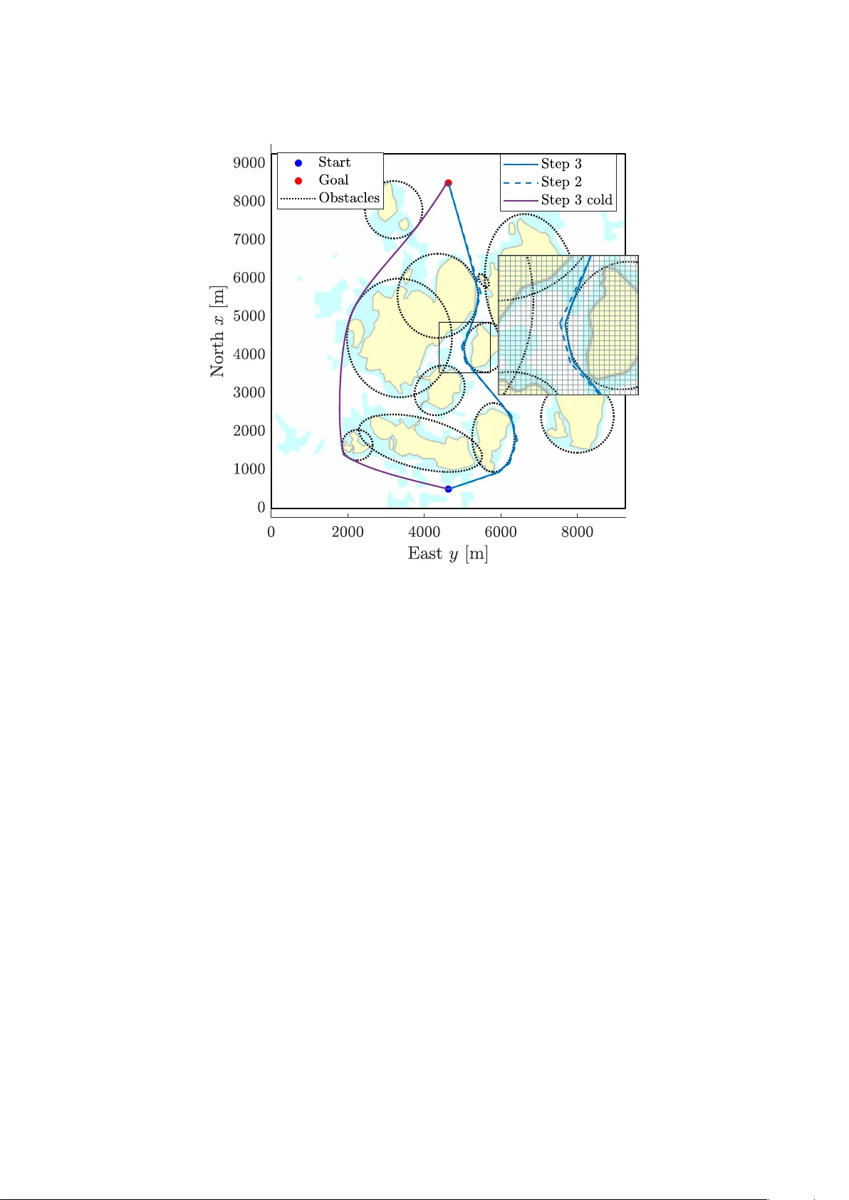
W arm-Started Optimized T ra jectory Planning for ASVs Glenn Bitar, V egard N. V estad, Anastasios M. Lekk as and Morten Breivik The authors are with the Centre for Autonomous Marine Operations and Systems, Department of Engineering Cybernetics, Norwegian Universit y of Science and T echnology (NTNU), NO-7491 T rondheim, Norw ay . E-mails: { glenn.bitar,anastasios.lekk as } @n tnu.no, vegardnitterv estad@gmail.com, morten.breivik@ieee.org c  2019 IF AC Abstract W e consider w arm-started optimized tra jectory planning for autonomous sur- face vehicles (ASVs) by combining the adv antages of tw o types of planners: an A ? implemen tation that quickly finds the shortest piecewise linear path, and an optimal con trol-based tra jectory planner. A nonlinear 3-degree-of-freedom under- actuated mo del of an ASV is considered, along with an ob jective functional that promotes energy-efficient and readily observ able maneuvers. The A ? algorithm is guaran teed to find the shortest piecewise linear path to the goal position based on a uniformly decomposed map. Dynamic information is constructed and added to the A ? -generated path, and provides an initial guess for warm starting the optimal con trol-based planner. The run time for the optimal control planner is greatly re- duced by this initial guess and outputs a dynamically feasible and lo cally optimal tra jectory . 1 In tro duction Motiv ated by p oten tial for reduced costs, as w ell as safer and more environmen tally friendly op erations, tec hnology for autonomous surface v ehicles (ASVs) is being devel- op ed at a rapid pace. Sev eral commercial actors are spearheading the search for solutions for safe, collision-free and reliable autonomous op erations. Rolls-Ro yce and Finferries demonstrated the world’s first autonomous car ferry “F alco” in 2018 (Jallal, 2018), whic h na vigated autonomously b etw een t wo ports in Finland b y combining adv anced sensor tec hnology and collision av oidance algorithms. A prerequisite for safe and efficien t op eration is a well-functioning path or tra jectory planning method. Suc h a method is resp onsible for pro viding the ASV with a safe tra jectory that av oids static obstacles such as land and shallow waters. Dep ending on the t yp e of op eration, one might wan t to optimize the tra jectory for v arious ob jectives, suc h as energy efficiency , speed or tra jectory length. 1 Uniform decomp osition V oronoi diagram RR T PRM P on try agin’s principle Dynamic programming Pseudosp ectral metho ds Multiple sho oting metho ds Com binatorial metho ds Sampling-based metho ds Analytical metho ds Appro ximate metho ds Roadmap metho ds Optimal con trol-based metho ds Pip elined optimization F ast, global Optimal, feasible Figure 1: Categorization of some planning algorithms. Numerous path and tra jectory planning algorithms ha ve been researched and are a v ailable for marine applications. One ma y categorize these planning algorithms as b e- ing roadmap-based or optimization-based. Figure 1 giv es an o verview of the categoriza- tion of some planning algorithm types. R o admap metho ds are based on exploring p oints in the geometric space in order to build a path b etw een the start and goal positions. There are tw o sub categories in roadmap metho ds. Combinatorial methods decomp ose an obstacle map using a preferred strategy , and perform a search in the resulting graph. The decomp osition strategies include e.g. uniform grids, V oronoi diagrams and visibil- it y graphs. The com binatorial methods explore the entire geometric space. The graph searc h is often p erformed using A ? , whic h is an efficient and w ell-known search algo- rithm widely used to solve path planning problems (Hart et al., 1968). A ? guaran tees to find the shortest path when using an admissible heuristic function. Hybrid A ? extends the A ? algorithm b y generating dynamic tra jectories to connect no des, thus adding dy- namic information to the search (Dolgo v et al., 2010). As opp osed to com binatorial metho ds, sampling-b ase d metho ds randomly explores p oints in the map to build a path to w ards the goal. Probabilistic roadmap (PRM) is a sampling-based planning metho d that draws samples from the configuration space and connects them using a lo cal plan- ner (Ka vraki et al., 1996). A graph searc h algorithm is applied to find the minimum cost path from start to goal in the resulting graph. Rapidly-exploring random tree (RR T) is another sampling-based metho d which calculates input tra jectories b etw een randomly sampled p oin ts and connects them in a tree until the start and goal positions are con- nected (LaV alle, 1998). Although RR T uses a cost function, the metho d is not optimal and will lock into the first connection b et w een start and goal. V arious flav ors of RR T are developed to amend this, e.g. RR T ? (Karaman and F razzoli, 2011). This metho d con tin uously performs tree rewiring and has probabilistic completeness, but con v erges slo wly . The other group of planning metho ds con tains algorithms based on optimal c ontr ol . This group may further b e divided into analytical and appro ximate metho ds. Analytical metho ds suc h as P ontry agin’s principle are only able to find solutions in very simple 2 Shortest piecewise linear path T ra jectory (initial guess) Energy- optimized tra jectory Scenario Ship mo del Step 1 Step 2 Step 3 A ? T ra jectory generation Optimal con trol Figure 2: Pip elined path planning concept. cases and are generally unpractical. Approximate methods such as e.g. pseudosp ectral optimal con trol (Bitar et al., 2018; Ross and Karpenko, 2012) are highly sensitive to initial guesses of the solution and will conv erge to a local optimum close to this guess. Without a go o d initial guess, they also exp erience long run times and are sensitiv e to problem dimensionality . Zhang et al. (2018) plan tra jectories for parking autonomous cars b y combining h ybrid A ? with an optimal control-based metho d. Motiv ated by the same goals of ex- ploiting the strengths and mitigate the weaknesses of optimal control-based algorithms, w e here atte mpt to solve the long-term tra jectory planning problem for ASVs as a tran- scrib ed optimal control problem (OCP), and w arm start the solver using the smoothed solution of an A ? geometric planner. In this three-step pip elined approach, the A ? plan- ner swiftly provides a set of wa yp oints representing the shortest path as Step 1. This path is conv erted in to a full state tra jectory by adding artificial and nearly feasible tem- p oral information as Step 2. Step 3 takes this tra jectory and uses it as the initial guess for an OCP solv er, which finds an optimized tra jectory near the globally shortest path. The structure of this pip elined concept is illustrated in Figure 2. The method is an off-line global planner, which assumes that information ab out the map and en vironmen t is known a priori. The rest of this pap er is organized as follows: Section 2 presents the mathematical mo del of the ASV used in sim ulations and planning. Finding the wa ypoints describing the shortest path with A ? is describ ed in Section 3, and Section 4 explains how the A ? solution is conv erted to a tra jectory . Section 5 shows how the OCP is transcribed to an nonlinear program (NLP), whic h yields an optimized tra jectory when solved. Sim ulation scenarios and results are presented in Section 6, while Section 7 concludes the paper. 2 ASV mo deling and obstacles In (Lo e, 2008), a simple nonlinear 3-degree-of-freedom ship mo del is iden tified to ap- pro ximate the dynamics of the ASV Viknes 830. Without loss of generality for the metho d describ ed in this paper, w e use that mo del to p erform tra jectory planning. The mo del has the form ˙ η = R ( ψ ) ν (1a) M ˙ ν + C ( ν ) ν + D ( ν ) ν = τ ( u ) . (1b) 3 The p ose v ector η = [ x, y , ψ ] > ∈ R 2 × S con tains the ASV’s p osition and heading angle in the Earth-fixed North East Down (NED) frame. The v elo cit y vector ν = [ u, v, r ] > ∈ R 3 con tains the ASV’s b o dy-fixed v elo cities: surge, sw a y and y aw rate, resp ectively . The rotation matrix R ( ψ ) transforms the bo dy-fixed velocities to NED: R ( ψ ) =   cos ψ − sin ψ 0 sin ψ cos ψ 0 0 0 1   . (2) The matrix M ∈ R 3 × 3 represen ts system inertia, C ( ν ) ∈ R 3 × 3 Coriolis and centripetal effects, and D ( ν ) ∈ R 3 × 3 represen ts damping effects. The ASV is con trolled b y the con trol vector u = [ X , N ] > ∈ R 2 , whic h contains surge force and ya w moment. The con trol v ector is mapp ed to a force v ector τ ( u ) = [ X , 0 , N ] > . The ASV’s states are collected in the vector x = [ x, y , ψ, u, v , r ] > , and we collect the dynamic mo del (1) in the following compact form for notational ease in the remainder of the pap er: ˙ x = f ( x , u ) = " R ( ψ ) ν M − 1  − C ( ν ) ν − D ( ν ) ν + τ ( u )  # . (3) 3 Step 1: A ? path planner T o quickly find the global shortest collision-free path betw een a start and goal p osition, w e use an A ? implemen tation on a uniformly decomposed grid. The A ? implemen tation is standard, and details may b e found in e.g. (Hart et al., 1968). The search algorithm lo oks for collision-free paths betw een no des in the uniform grid, and uses Euclidean distance as cost and heuristic functions. The decomp osition of the map affects the solution space and the run time for Step 1. Using a uniform grid with grid size ∆ d > 0 to o large will tak e paths going through narro w passages aw ay from the solution space, and the desired shortest path may not b e found. A smaller grid size will explore more options, but requires more ev aluation, giving a longer run time. This uniform grid is in our case chosen for simplicit y , ho w ev er exploring other decomp ositions suc h as V oronoi diagrams or a non-uniform grid migh t b e desirable for p erformance reasons. 4 Step 2: T ra jectory generation In order to use the shortest path generated b y Step 1 as an initial guess for the OCP, w e conv ert it to a tra jectory based on straight segmen ts and circle arcs using a nom- inal forw ard velocity u nom > 0. The tra jectory generation consists of three sub-steps: w a yp oin t reduction, w a ypoint connection, and adding dynamic information. 4.1 W aypoint reduction Algorithm 1 is emplo y ed to reduce the A ? path from Step 1 to a minimum num b er of w aypoints. The algorithm outputs a reduced path as an ordered set of w aypoints P =  p k ∈ R 2 | k = 1 , . . . , N r  where N r is the num b er of w aypoints. The A ? w a yp oin ts are denoted p ? k for k = 1 , . . . , N ? , ordered from start to goal, where N ? is the num b er of wa yp oints. 4 Algorithm 1 W aypoint reduction algorithm. 1: procedure Reduce 2: i ← N ? ; P ← InitializePath ( p ? i ) 3: do 4: for j = 1 to i − 1 do 5: if ¬ Collision ( p ? i , p ? j ) then 6: AddPoint ( P , p ? j ) 7: i ← j 8: break 9: while i > 1 4.2 W aypoint connection The w aypoints in the reduced path p k ∈ P are connected with straight segments and circle arcs to increase geometric feasibilit y . This is done b y calculating the parameters of a circle based on a radius of acceptance R acc > 0. The result is a path with discontin uous turn rate since the turn rate of such a curv e will exp erience jumps at the b eginning and end of the circle arcs. Ho wev er, if the circle arcs hav e a turning radius R turn > 0 larger than the minim um turning radius of the ASV R turn , min > 0, the resulting geometry of the path can be follow ed tightly . Additional information about such a path wa ypoint connection is a v ailable in (F ossen, 2011). F or eac h straigh t segmen t, the turn rate is 0. F or the circle arcs, the turn rate is u nom / R turn ,k , where R turn ,k > 0 is the turning radius for arc k . The tangent angles for the straigh t segmen ts are γ k ∈ S, and for the circle arcs, the tangen t angles mo v e b et w een γ k and γ k +1 , dep ending on ho w far along the curve it is ev aluated. Using this information, w e can concatenate a path c onsisting of alternations of straigh ts and circle arcs, and construct a path function parametrized by length with p osition p g : [0 , L path ] → R 2 , (4a) where L path > 0 is the total length of the path. F unctions for path tangential angle and turn rate are also constructed: γ g : [0 , L path ] → S , and (4b) r g : [0 , L path ] → R , (4c) resp ectiv ely . These functions are subscripted b y ( · ) g to indicate that they are based on the path geometry . 4.3 Adding temp oral information After obtaining an arc-length parametrized path w e add temporal information b y as- suming a constant surge velocity u nom , a swa y velocity v of zero, and piecewise constan t y a w rate r . The nominal surge velocity is determined by u nom = L path t max , where t max > 0 is the tunable time to complete the tra jectory , whic h is v alid on t ∈ [0 , t max ]. The distance 5 tra v eled will be L ( t ) = u nom · t , and the states will then ha v e tra jectories  x w ( t ) y w ( t )  > = p g ( L ( t )) (5a) ψ w ( t ) = γ g ( L ( t )) (5b) u w ( t ) = u nom (5c) v w ( t ) = 0 (5d) r w ( t ) = r g ( L ( t )) . (5e) The input tra jectory is set to the constant v alues τ X,w ( t ) = τ X,ss , τ N ,w ( t ) = 0 (6) where τ X,ss ∈ R is calculated as the steady-state v alue required to maintain nominal forw ard velocity u nom . The tra jectories are subscripted by ( · ) w to indicate that they will b e used for warm-starting the OCP in Step 3. The resulting tra jectory is not dynamically feasible according to (1) but will b e used as an initial guess for the OCP solver, describ ed in the next section. The tra jectory is collected in the follo wing vectors: x w ( t ) =         x w ( t ) y w ( t ) ψ w ( t ) u w ( t ) v w ( t ) r w ( t )         u w ( t ) =  τ X,w ( t ) τ N ,w ( t )  ∀ t ∈ [0 , t max ] . (7) The goal of the method describ ed in this pap er is to find a tra jectory of states and inputs that minimizes a cost functional J ( x ( · ) , u ( · )): J ( x ( · ) , u ( · )) = Z t max 0 F ( x ( τ ) , u ( τ )) d τ , (8) whic h is dependent on a cost-to-go function F ( x , u ). This function may be selected to find e.g. the tra jectory that minimizes energy usage. The initial guess for the cost tra jectory J w ( · ) at time t is determined by J w ( t ) = Z t 0 F ( x w ( τ ) , u w ( τ )) d τ . (9) 5 Step 3: Optimal con trol Optimal con trol is used to mak e feasible and optimize the tra jectory provided b y Step 2. An OCP is form ulated as min x ( · ) , u ( · ) Z t max 0 F ( x ( τ ) , u ( τ )) d τ (10a) sub ject to ˙ x ( t ) = f ( x ( t ) , u ( t )) ∀ t ∈ [0 , t max ] (10b) h ( x ( t ) , u ( t )) ≤ 0 ∀ t ∈ [0 , t max ] (10c) e ( x (0) , x ( t max )) = 0 . (10d) The solution of this OCP gives a tra jectory of states x ( · ) and inputs u ( · ) that minimizes (8). 6 5.1 Cost functional The cost functional describ ed in (8) is dep endent on the cost-to-go function F ( x , u ). This function may be adjusted and structured according to the desired sense of optimal- it y . Our aim is a tra jectory which is optimized for energy usage, as w ell as p erforming readily observ able maneuv ers, as is required b y In ternational Regulations for Prev enting Collisions at Sea (COLREGs) Rule 8. This results in a tw o-part cost-to-go function: F ( x , u ) = K e F e ( x , u ) + K t F t ( x ) , (11) with tuning parameters K e , K t > 0. The first term p enalizes energy usage and describ es w ork done b y the actuators: F e ( x , u ) = | u · τ X | + | r · τ N | . (12) The second term is a disprop ortionate penalization on turn-rate r , whic h prefers readily observ able turns p erformed with high turn-rate. The function has the form F t ( x ) =  a t r 2 + (1 − e − r 2 b t )  1 F t,max , (13) where F t,max = a t r 2 max + (1 − e − r 2 max b t ) , (14) and r max > 0 is the ASV’s maxim um y aw rate. The tuning parameters a t > 0 and b t > 0 shap e the penalization to prefer higher or low er turn-rate, which is an idea obtained from (Eriksen and Breivik, 2017). 5.2 Obstacles Obstacles are enco ded as elliptic inequalities in (10c). The basis for one elliptic obstacle is  x − x c x a  2 +  y − y c y a  2 ≥ 1 , (15) where x c and y c describ e the ellipse cen ter and x a and y a describ e the sizes of the tw o elliptic axes. The ellipses are rotated by α , whic h is the angle b etw een the global x -axis and the direction of x a . The resulting inequalit y b ecomes g o ( x, y , x c , y c , x a , y a , α ) = − log   ( x − x c ) cos α + ( y − y c ) sin α x a  2 +  − ( x − x c ) sin α + ( y − y c ) cos α y a  2 +   + log(1 +  ) ≤ 0 , (16) where a small v alue ε > 0 is added to deal with feasibility issues as x → x c and y → y c , and the logarithmic function is used to reduce n umerical sizes, without changing the inequalit y . The same function is used in (Bitar et al., 2019). 7 5.3 NLP transcription A multiple-shooting approac h is used to transcrib e the OCP into an NLP: min w φ ( w ) (17a) sub jec t to g lb ≤ g ( w ) ≤ g ub (17b) w lb ≤ w ≤ w ub . (17c) The dynamics are discretized in to N ocp steps in time, with step length h = t max / N ocp . The decision v ariables w consist of the s tate v ariables x k = x ( t k ) , k = 0 , 1 , . . . , N ocp , the accumulated costs J k = J ( t k ) , k = 0 , 1 , . . . , N ocp , where J ( t ) = Z t 0 F ( x ( τ ) , u ( τ )) d τ , (18) and the con trol inputs u k = u ( t k ) , k = 0 , 1 , . . . , N ocp − 1: w = h z > 0 u > 0 z > 1 . . . u > N ocp − 1 z > N ocp i > , (19) where z k = [ x > k , J k ] > . The cost function (17a) approximates (10a) and is φ ( w ) = J N ocp . (20) The constraints (17b) are used to satisfy shooting constraints, as well as the collision a v oidance constraints. F or the shooting constraints, w e construct a discrete representa- tion of the dynamics (10b) as well as the integral (18) using a RK4 sc heme with K ocp steps. W e define the discrete v ersion of (10b) augmen ted with the time deriv ativ e of (18) as z k +1 = F ( z k , u k ) , (21) and construct the sho oting constraints g s ( w ) =     z 1 − F ( z 0 , u 0 ) . . . z N ocp − F ( z N ocp − 1 , u N ocp − 1 )     , (22) with asso ciated lo wer and upp er bounds g s,lb = g s,ub = 0 ( n +1) · N ocp . (23) F or obstacles i = 1 , 2 , . . . , N o , w e a void collisions by satisfying the inequalit y con- strain t g o ( x k , y k , x c,i , y c,i , a i , b i , α i ) ≤ 0 , (24) where x k = x ( t k ) and y k = y ( t k ) for k = 1 , 2 , . . . , N ocp . W e create a v ector for all our obstacles in a single time step: ¯ g o ( x k ) =       g o ( x k , y k , x c, 1 , y c, 1 , a 1 , b 1 , α 1 ) g o ( x k , y k , x c, 2 , y c, 2 , a 2 , b 2 , α 2 ) . . . g o ( x k , y k , x c,N o , y c,N o , a N o , b N o , α N o )       . (25) 8 Obstacle constraints for all time steps are gathered in g o ( w ) =       ¯ g o ( x 0 ) ¯ g o ( x 1 ) . . . ¯ g o ( x N ocp − 1 )       (26) with asso ciated lo wer and upp er bounds g o,lb = − ∞ N o · N ocp and g o,ub = 0 N o · N ocp . (27) The nonlinear inequalit y constraints (17b) are completed as g lb =  g s,lb g o,lb  , g ( w ) =  g s ( w ) g o ( w )  , g ub =  g s,ub g o,ub  . (28) The decision v ariable b ounds (17c) are used to satisfy constant state and input constrain ts, as w ell as b oundary conditions (10d). The bounds are w > lb = h z > s,lb u > lb z > lb u > lb . . . u > lb z > f ,lb i (29a) w > ub = h z > s,ub u > ub z > ub u > ub . . . u > ub z > f ,ub i , (29b) where z s,lb =  x s y s ψ lb u r,s 0 0 0  > (30a) z s,ub =  x s y s ψ ub u r,s 0 0 0  > (30b) z f ,lb =  x f y f ψ lb u r,lb 0 0 0  > (30c) z f ,ub =  x f y f ψ ub u r,ub 0 0 ∞  > (30d) z lb =  x lb y lb ψ lb u r,lb v lb r lb 0  > (30e) z ub =  x ub y ub ψ ub u r,ub v ub r ub ∞  > (30f ) u lb =  X lb N lb  > (30g) u ub =  X ub N ub  > , (30h) and where v alues subscripted with ( · ) s represen t initial conditions, ( · ) f the final condi- tions, and ( · ) lb and ( · ) ub represen t low er and upp er b ounds, respectively . 5.4 Initial guess and solv er The tra jectories x w ( · ), u w ( · ) and J w ( · ) from Section 5.4 are used as an initial guess to w arm-start the NLP. These tra jectories are sampled at the time steps t k , k = 0 , . . . , N ocp using interpolation, and shap ed into the form of the decision v ector w (19), pro viding the initial guess w 0 . The NLP as defined by (17) is solved by the interior-point metho d Ipopt (W¨ ac h ter and Biegler, 2005) using Casadi (Andersson et al., 2018) for Matlab. 9 T able 1: Algorithm step explanation. Step Parametrized by Dynamic feasibility Optimalit y 1 Length None, piecewise linear Shortest piecewise linear path 2 Time Discon tin uous y a w rate r None 3 Time Adheres to (1) Energy and COLREGs Rule 8 T able 2: P arameter v alues. P aram. V al. P aram. V al. ∆ d 50 [m] t max 2200 [s] N ocp 1000 K ocp 1 K e 3 . 5 · 10 − 4 [J − 1 ] K t 800 a t 112 [s 2 / rad 2 ] b t 6 . 25 · 10 − 5 [rad 2 / s 2 ] R acc 10 [m] R turn , min 24 . 5 [m] r max 40 [ ◦ / s] 5.5 Algorithm summary The pip elined algorithm is summarized b y the steps in T able 1, where the prop erties of eac h step are highligh ted in terms of parametrization, feasibility according to (1) and optimalit y . While Step 1 gives the shortest piecewise linear path, it is parametrized b y length, and will not b e dynamically feasible for warm-starting the OCP in Step 3. Step 2 connects the w aypoints with circle arcs and adds artificial dynamics, which mo v es us closer to a dynamically feasible tra jectory . Ho w ever, w e lose the optimality of the shortest path with this mo dification, and the y aw rate is discontin uous, which is not p ossible according to (1). This tra jectory is usable as an initial guess for Step 3, whic h con v erges to a tra jectory that adheres to (1), and adds optimality according to (10a). 6 Sim ulation scenarios and results The scenario selected for testing our planning method is Sjernarøy north of Stav anger, Norw a y , near 59 . 25 ◦ N and 5 . 83 ◦ E. A map of this scenario is sho wn in Figure 3. The scenario has many possible routes b etw een the start and goal p ositions, including routes that go outside the islands, and the narrow passage b et w een the islands. The narrow passage is the shortest path, and one could claim that in the absence of disturbances, this shortest path is also the most energy efficien t. Ho w ever, since the problem of finding this path is non-con vex and resem bles an integer problem, the OCP alone w ould struggle to find the shortest path. W e use the algorithm parameters presen ted in T able 2. T o b enc hmark our planning algorithm, w e apply it to the scenario illustrated in Figure 3 in Matlab on a laptop with an Intel Core i7-7700HQ pro cessor. F or comparison, w e also apply the OCP to the same scenario without an initial guess, i.e. cold starting Step 3. Solutions from these tw o metho ds will b e dynamically feasible tra jectories with differen t routings to reach the goal p osition. W e use metrics of total cost and run times to compare the algorithms. These metrics will also b e applied to the tra jectory after Step 2. This tra jectory is not dynamically feasible according to (1) but can tell us how 10 Figure 3: Map showing the scenario used for planning, with m ultiple elliptical obstacle b oundaries surrounding the small islands. T ra jectories after steps 2 and 3 are plotted. A cold-started solution is also included. the smo othed A ? tra jectory p erforms without optimization. The resulting tra jectories are plotted on top of the scenario in Figure 3. W e see that the initial guess go es through the narrow passage b et w een the islands and that the w arm-started OCP finds a solution along the same route. As exp ected, the cold-started OCP goes outside the passage and finds a longer solution. A zo omed inset in Figure 3 sho ws ho w the OCP is able to pro duce readily observ able maneuvers by making sharp turns around the obstacle b oundaries. The inset also includes the grid used b y Step 1. Figure 4 shows us the cost functional dev elops along the tra jectories of the w arm- started OCP ( K e · J e + K t · J t ), the initial guess ( J w ) and the cold-started OCP ( J c ). T able 3 shows the results at t = t max for the three metho ds. W e see the scaled total cost as calculated by (10a) and (11), as w ell as the energy cost calculated b y (12). An impro v ement of 30 % is obtained by warm-starting the OCP compared to cold starting it, explained by the shorter route selection. The w arm-started OCP is also able to impro v e on the dynamically infeasible initial guess by 4 %. T able 3 also shows the run times of the three metho ds. Since the initial guess alone do es not p erform any iterative optimization, it has the low est run time. The w arm-started metho d sp ends 27 s in total to find an optimized solution to the path planning problem, including 21 s sp ent solving the OCP. This is an improv ement of 84 % compared to the cold-started OCP which spends approximately three minutes. 11 Figure 4: Cost functional dev elopmen t along both the optimized tra jectory and the initial guess. The optimized tra jectory shows the cost split into con tributions from energy optimization and observ able maneuv ers. Also, the cost of the cold-started OCP is denoted J c . T able 3: Scenario results. W arm started Step 3 Cold started Step 3 Step 2 F easible Y es Y es No Scaled total cost ( J ) 1 . 08 · 10 4 1 . 54 · 10 4 1 . 13 · 10 4 Unscaled energy cost ( J e ) 2 . 74 · 10 7 [J] 3 . 94 · 10 7 [J] 2 . 84 · 10 7 [J] T otal run time 26 . 7 [s] 174 [s] 5 . 7 [s] Step 1 run time 3 . 4 [s] - 3 . 4 [s] Step 2 run time 2 . 2 [s] - 2 . 2 [s] Step 3 run time 21 . 1 [s] 174 [s] - Step 3 iterations 58 549 - The run-time cost of obtaining a feasible tra jectory via optimal con trol is significan t compared to performing A ? and dynamic generation alone. The state tra jectories for the initial guess and warm-started OCP are sho wn in Figure 5. F rom the heading angle plot, w e see that ψ p erforms jumps of more than 30 ◦ , whic h is a clear indication of inten t to other vessels, even in situations with restricted visibilit y (Cock croft and Lameijer, 2004). This is further observed in the y a w rate state r , where instead of ha ving long turns with lo w ya w rate magnitude, we ha ve abrupt turns with high-v alued r . This is shown more clearly in Figure 6, which zo oms in on a selected time in terv al. 7 Conclusion W e ha v e dev elop ed and demonstrated a pipelined tra jectory planning algorithm that exploits the speed and global prop erties of an A ? searc h with the optimalit y of an 12 Figure 5: State v alues for heading, velocities and ya w rate for b oth the optimized tra jectory and the initial guess. OCP solver. The results from Section 6 show that using the initial guess provided by a smo othed A ? path in an OCP significantly improv es both run time and optimalit y compared to a cold-started OCP alone. Performing optimization on the A ? path signif- ican tly increases run time but will find a feasible lo cally optimal tra jectory , as opp osed to A ? alone. Qualitativ ely , the developed metho d is complete in terms of the shortest p ath , since this is the geometric ob jective of the A ? implemen tation. This is dep enden t on the discretization of the map, since using larger grid spacing to reduce run time remo v es narro w passages from the solution space. Using a different discretization sc heme such as e.g. V oronoi diagrams may guarantee a complete solution space. The dev elop ed metho d is also locally optimal in the sense of the pro vided ob jective, which is a com bination of energy consumption and readily observ able maneuvers in our case. The optimality is pro vided by the implemented OCP which alone is not able to find the global optim um, demonstrated by the cold-started result in Figure 3. How ever, the OCP w arm-started b y the shortest path found b y the A ? metho d is at least lo cally optimal and may b e close to the global optim um, since, in the absence of disturbances, the shortest path is also the one that requires the least energy . In addition to improving optimality of the A ? result, the OCP adds feasibility , unlik e the A ? consideration which is purely geometric. Using this warm-starting sc heme is that the OCP will lo ck into one routing alternativ e. Dep ending on the desired sense of optimalit y , this may not b e the desired solution, which is a disadv an tage to some use cases. 13 Figure 6: Zo omed-in section of Figure 5. The algorithm presen ted here has been used in a hybrid collision av oidance arc hitec- ture in (Eriksen et al., 2019), where it is extended to include disturbances in the form of o cean c urren ts. F urther w ork on this topic includes: • Implemen ting a more general obstacle representation to handle a wider range of map represen tations. E.g. the obstacle represen tation in (Zhang et al., 2018) han- dles conv ex p olygons as smo oth inequalit y conditions. • Impro vemen ts on the map discretization scheme are also desirable to reduce com- putational time of the A ? algorithm while preserving completeness of the solution space. • Additionally , an OCP representation that is parametrized by straigh t lines b e- t w een wa ypoints in combination with full-state dynamics may b e adv antageous to inheren tly pro duce COLREGs-complian t tra jectories. Ac knowledgemen ts This w ork is funded by the Research Council of Norwa y and Innov ation Norwa y with pro jec t num b er 269116. The w ork is also supp orted b y the Centres of Excellence funding sc heme with pro ject n um ber 223254. 14 References Andersson, J. A. E., Gillis, J., Horn, G., Rawlings, J. B., and Diehl, M. (2018). CasADi – A soft ware framew ork for nonlinear optimization and optimal con trol. Mathematic al Pr o gr amming Computation , 11(1):1–36. Bitar, G., Breivik, M., and Lekk as, A. M. (2018). Energy-optimized path planning for autonomous ferries. In Pr o c. of the 11 th IF A C CAMS, Op atija, Cr o atia , pages 389–394. Bitar, G., Eriksen, B.-O.H., Lekk as, A. M., and Breivik, M. (2019). Energy-optimized h ybrid collision a v oidance for ASVs. In Pr o c. of the 17 th ECC, Naples, Italy . Co c k croft, A. N. and Lameijer, J. N. F. (2004). A Guide to the Col lision Avoidanc e R ules . Elsevier Butterworth-Heinemann. Dolgo v, D., Thrun, S., Montemerlo, M., and Diebel, J. (2010). Path planning for autonomous v ehicles in unkno wn semi-structured en vironmen ts. The International Journal of R ob otics R ese ar ch , 29(5):485–501. Eriksen, B.-O.H., Bitar, G., Breivik, M., and Lekk as, A. M. (2019). Hybrid collision a v oidance for ASVs complian t with COLREGs rules 8 and 13–17. [eess.SY]. Submitted to F r ontiers in R ob o tics and AI . Eriksen, B.-O.H. and Breivik, M. (2017). MPC-based mid-level collision av oidance for ASVs using nonlinear programming. In Pr o c. of the IEEE CCT A, Mauna L ani, HI, USA , pages 766–772. F ossen, T. I. (2011). Handb o ok of Marine Cr aft Hydr o dynamics and Motion Contr ol . Wiley-Blac kw ell. Hart, P ., Nilsson, N., and Raphael, B. (1968). A formal basis for the heuristic determina- tion of minimum cost paths. IEEE T r ansactions on Systems Scienc e and Cyb ernetics , 4(2):100–107. Jallal, C. (2018). Rolls-Royce and Finferries demonstrate world’s first fully autonomous ferry . Maritime Digitalisation & Communic ations . Accessed 2019-04-11. Karaman, S. and F razzoli, E. (2011). Sampling-based algorithms for optimal motion planning. The International Journal of R ob otics R ese ar ch , 30(7):846–894. Ka vraki, L. E., Sv es tk a, P ., Latombe, J.-C., and Ov ermars, M. H. (1996). Probabilistic roadmaps for path planning in high-dimensional configuration spaces. IEEE T r ans- actions on R ob otics and Automation , 12(4):566–580. LaV alle, S. M. (1998). Rapidly-exploring random trees: A new to ol for path planning. T echnical rep ort. Lo e, Ø. A. G. (2008). Collision a voidance for unmanned surface vehicles. Master’s thesis, Norw egian Universit y of Science and T echnology , T rondheim, Norwa y . Ross, I. M. and Karp enk o, M. (2012). A review of pseudospectral optimal control: F rom theory to fligh t. A nnual R eviews in Contr ol , 36(2):182–197. 15 W¨ ac hter, A. and Biegler, L. T. (2005). On the implemen tation of an in terior-p oin t filter line-searc h algorithm for large-scale nonlinear programming. Mathematic al Pr o gr am- ming , 106:25–57. Zhang, X., Liniger, A., Sak ai, A., and Borrelli, F. (2018). Autonomous parking using optimization-based collision av oidance. In Pr o c. of the IEEE CDC, Miami Be ach, FL, USA , pages 4327–4332. 16