Resolution analysis in a lens-free on-chip digital holographic microscope

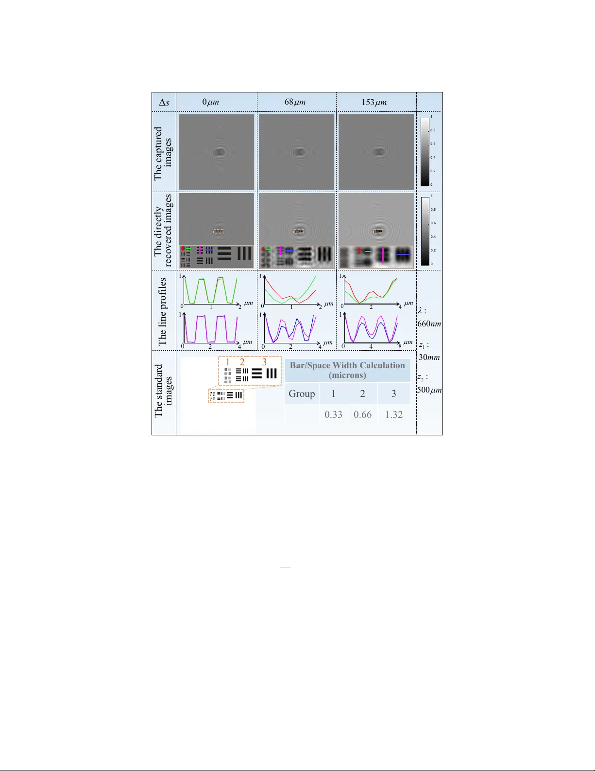
R e s o l u t i o n a n a l y s i s in a l e n s - f r e e o n- ch ip di gi ta l h o l o g r a p h i c m ic ros co pe J I A L I N Z H A N G , 1 , 2 , 3 J I A S O N G S U N , 1 , 2 , 3 Q I A N C H E N , 2 , 4 A N D C H A O Z U O 2 , 3 , * 1 Sc hool of Electronic and Op tical Engineering, N anjing U niv ersity of Science and T ec hnology, N o. 200 Xiaolingw ei Str ee t, Nanjing, Jiangsu Pr o vince 210094, China 2 Jiangsu Key Labor atory of Spectral Imaging & Int ellig ent Sense, N anjing, Jiangsu Pr ovince 210094, China 3 Smart Computational Imaging Laboratory (SCILab), Nanjing U niv er sity of Science and T echnology , Nanjing, Jiangsu Pr o vince 210094, China 4 c henq@njust.edu.cn * zuochao@njus t.edu.cn Abstract : Lens-free on-chip digital holographic microscopy (LFOCDHM) is a modern imaging technique whereby the sample is placed directly onto or very close to the digital sensor , and illuminated b y a partially coherent source located f ar abo v e it. The scattered object wa v e interf eres with the ref erence (unscattered) wa v e at the plane where a digital sensor is situated, producing a digital hologram that can be processed in sev eral w a y s to extract and numer icall y reconstruct an in-f ocus image using the back propagation algor ithm. Without requiring any lenses and other intermediate optical components, the LFOCDHM has unique advantag es of offer ing a large effectiv e numer ical aper ture (NA) close to unity across the native wide field-of-vie w (FO V) of the imaging sensor in a cost-effectiv e and compact design. Ho we ver , unlike con v entional coherent diffraction limited imaging systems, where the limiting aper ture is used to define the system performance, typical lens-free microscopes only produce compromised imaging resolution that far belo w the ideal coherent diffraction limit. At least five major factors may contr ibute to this limitation, namely , the sample-to-sensor distance, spatial and temporal coherence of the illumination, finite size of the equally spaced sensor pixels, and finite extent of the image sub-FO V used f or the reconstruction, which hav e not been sys tematically and r igorousl y explored until no w . In this work, we der iv e fiv e transfer function models that account for all these phy sical effects a nd interactions of these models on the imaging resolution of LFOCDHM. W e also e xamine how our theoretical models can be utilized to optimize the optical design or predict the theoretical resolution limit of a given LFOCDHM system. W e present a ser ies of simulations and experiments to confir m the v alidity of our theoretical models. © 2019 Optical Society of America 1. Introduction High-throughput optical microscop y is essential to v arious biomedical applications such as cell cy cle assay , dr ug dev elopment, digital pathology , and high-content biological screening [1, 2]. For con ventional whole slide imaging (W SI) sys tems, in order to capture a high-throughput image with both high-resolution and large field of vie w (FO V), mechanical scanning and stitching are required to e xpand the limited FO V of a con v entional high magnification objectiv e [3], which not only complicate the imaging process, but also significantly inc rease the ov erall cost of the sy stem. The recently dev eloped computational microscop y techniques provide new oppor tunities to create high-resolution wide FO V imag es without any mechanical scanning and stitching, such as synthetic aper ture inter f erometr ic microscopy [4 – 9], Fourier ptyc hog raph y microscopy (FPM) [10 – 16], and lens-free on-chip microscopy [17 – 20]. Among these approaches, the lens-free on-chip microscopy has unique advantag es of achie ving a larg e effective numer ical aper ture (NA) ∼ 1 across the nativ e FO V of the imaging sensor tens of mm 2 , based on a so-called unit-magnification configuration, where the samples are placed as close as possible to the imaging sensor [21, 22]. W ithout requir ing any lenses and other optical components between the object and the sensor planes, lens-free on-chip microscopy allow s to significantly simplify the imaging sys tem and meanwhile effectivel y circumv ent the optical aber rations and chromaticity that are ine vitable in con v entional lens-based imaging systems [23, 24]. There are two typical designs f or a lens-free on-chip microscope, so-called contact-mode shado w imaging-based microscope [17, 25] and lens-free on-chip digital holographic microscope (LFOCDHM) [21, 26]. In the contact-mode shado w imaging-based microscopes, the distance betw een the sample and the sensor need to be quite small (typically less than 10 µ m ), and the captured shado ws of the objects can be regarded as a two-dimensional absor ption image of the specimen [27]. Ho we v er, the small distance is v er y difficult to achie v e in practice due to the e xistence of protectiv e glass cov er ing the surface of the camera sensor . In LFOCDHM, the distance between the objects and the sensor chip can be sizeable, and diffraction patterns are generated from the inter f erence betw een the scattered light from each object and itself or the unscattered background light. The diffraction patter ns are be digitally processed to reconstruct an image of the specimen, and the associated twin-image artifacts need to be eliminated or par tiall y remo ved relying on computational phase retriev al algorithm [28, 29]. In the f ollo wing analy sis, we will ex amine LFOCDHM ex clusiv el y . Despite the advantag es mentioned earlier , the LFOCDHM systems generall y suffer from lo w imaging resolution which is far from enough to meet the demand of recent biomedical research, particularly with respect to the visualization of cellular or subcellular details of biological structures and processes. U nlike conv entional coherent diffraction limited imaging systems, where the limiting aper ture is used to define the sys tem per f ormance, typical LFOCDHM systems only produce compromised imaging resolution that far below the ideal coherent diffraction limit. A ccording to Nyquist-Shannon sampling theorem, the resolution of the holographic reconstruction is fundamentally limited to the sampling resolution of the imaging devices since the recorded holographic fr ing es are not magnified. In other words, the phy sical pix el-size is one important limiting factor of these lens-free imaging systems [27]. Because of the spatial aliasing/undersampling, the imaging sensor will fail to record holographic oscillation corresponding to high spatial frequency inf or mation of the specimen. T o address this problem, pix el super-resolution (SR) methods hav e been proposed in which the holog ram with a smaller effectiv e pixel size can be synthesized from multiple low -resolution (LR) measurements through specific computational algor ithms [17, 18, 25, 26, 30]. With these pix el SR methods, the imaging resolution of the LFOCDHM systems can be impro v ed from Nyquist-Shannon limit (half-pitch lateral resolution of ∼ 2 µ m , effective NA of ∼ 0 . 1 − 0 . 2 ) to an effectiv e numerical aperture of ∼ 0 . 4 − 0 . 5 [17, 18, 26, 31]. Ev en though the achiev ed imaging resolution is still onl y less than half of the ideal coherent diffraction limit (NA ∼ 1 ). The reason f or this is that besides the pix el size of the sensor, at least 4 additional factors act to significantly limit the per f or mance of LFOCDHM sy stems, namely , the sample-to-sensor distance, spatial and temporal coherence of the illumination, and finite e xtent of the image sub-FO V used f or the reconstruction. This is not une xpected and has been discussed b y other authors see, f or example, Ref s. [18, 27]. How ev er , either only qualitative analy ses were presented [32, 33], or only one or tw o of these factors on the imaging resolution hav e been considered [33 – 36]. In these quantitativ e analy ses [34 – 36], the discrete features of the sensor attract more attention, bu t the other basic parameters, e.g., the sample-to-sensor distance [37], spatial and temporal coherence of the illumination [33], and finite e xtent of the imag e sub-FO V [38], are sporadically mentioned in the off-axis/in-line digital holographic microscopy . Thus, the influence of these 5 factors on the imaging resolution of LFOCDHM has not been systematicall y e xamined and r igorousl y explored until no w . In this w ork, w e ha v e conducted a systematical research on the effect of five major factors on imaging resolution of a LFOCDHM system, i.e., the sample-to-sensor distance, spatial and temporal coherence of the illumination, finite size of the equally spaced sensor pixels, and finite e xtent of the image sub-FO V used f or the reconstruction. W e derive fiv e transfer function models that account for all these ph y sical effects and their interactions on the imaging resolution of LFOCDHM. W e fur ther combine all these effects into a unified transfer function, which is the continued multiplication of the fiv e sub-transfer functions. W e e xamine ho w these theoretical models can be utilized to predict the theoretical resolution limit of a given LFOCDHM system or provide a useful guide to the selection of different system parameters f or the optimization of the imaging resolution when designing a ne w LFOCDHM system. A ser ies of simulations and e xper iments are presented to confir m the validity of our theoretical models. 2. Principle 2.1. T ypical optical setup f or LFOCDHM In the lens-free holog raphic microscope as depicted in Fig. 1(a), the source can simply be a laser [20, 39, 40], a LED (an ar ra y of LEDs) [41 – 44] or ev en a smar tphone screen [17]. The coherent or par tiall y coherent light illuminates the specimen, and then the scattered light and the transmitted light co-propagate in the same direction, finally f or ming inter f erence fringes on the imaging device. In the ideal case, the sample should be placed on a sensor ar ra y which can directl y capture the shadow s of the objects and av oid the twin-image ar tif acts. How ev er , due to the e xistence of protectiv e glass cov er ing the sur f ace of the camera sensor , there is usually alwa ys a cer tain distance betw een the sample plane and the detector plane (typically 0 . 3 − 2 mm ) [22, 26, 45]. Since the distance is much larger than the wa v elength, and the object inf or mation (including both amplitude and phase) is encoded into the diffraction patter ns, which needs to be computationally reconstructed b y phase retr ie val and numer ical back propagation algorithms. As illustrated in the schematic diagram Fig. 1(b) of the lens-free holographic microscope, neglecting the noise effect, the achie vable resolution of LFOCDHM is deter mined b y the maximum visualized radius R of the diffraction patter ns, which ref er to the cut-off frequency of the transfer function. This transfer function can be fur ther decomposed into five sub transf er functions, and the least cut-off frequency of the fiv e transf er functions limits the maximum Source a 1 z 2 z b p ∆ L ∆ Extended light source: ; ; λ λ ∆ s ∆ 2 z 1 z R Fig. 1. Lens-free on-chip imaging. (a) General lens-free imaging e xperimental setup based on complementary metal-oxide semiconductor (CMOS) or charg e-coupled device (CCD) image sensors. (b) Schematic of a lens-free holog raphic microscope. The sample is illuminated with wa velength λ , the spectral width ∆ λ , the diameter of the light-emitting area ∆ s . The diffraction patter n is registered by a sensor with pitch ∆ p at a distance z 2 . imaging resolution of LFOCDHM. The fiv e sub transfer functions respectivel y cor respond to the impact of the defocus distance, the limited temporal coherence length (the spectral width ∆ λ ), the spatial coherence length (the diameter of light-emitting area ∆ s ) of the source, the finite pixel size ( ∆ p ), and the finite e xtent of the image sub-FO V used f or the reconstruction (the side length ∆ L ). The absor ption and phase transfer functions resulting from propagation are respectivel y denoted as A T F P and PT F P . Then the temporal coherence transfer function, the spatial coherence transf er function, pixel size transf er function, the reconstructed region transf er function are sev erally expressed as T CT F , SC T F , P ST F , R RT F . Here, the latter f our sub-transf er functions are mutually independent, and together ha ve impacts on the final imaging results. 2.2. Theoretical analysis of resolution in LFOCDHM 2.2.1. Influence of sample-to-sensor distance on imaging resolution In this subsection, we adopt the weak object appro ximation to simplify the mathematical f or mulation and linear ize the phase retr ie val problem [46, 47]. The complex transmittance of a w eak object can be represented as t ( x ) = a ( x ) e i φ ( x ) ≈ a ( x ) [ 1 + i φ ( x )] a ( x ) = a 0 + ∆ a ( x ) ≈ a 0 + ∆ a ( x ) + i a 0 φ ( x ) , (1) where a ( x ) is the absor ption distribution with a mean value of a 0 , φ ( x ) is the phase distribution, x represents the two-dimensional coordinate (x,y) in spatial domain. T aking Fourier transf or m of both sides of Eq. 1, the Fourier spectr um of t ( x ) can be obtained as T ( u ) = a 0 δ ( u ) + A ( u ) + i a 0 Φ ( u ) , (2) where u is the two-dimensional coordinate in frequency domain, δ ( u ) is the Dirac Delta function, A ( u ) and Φ ( u ) respectiv ely represent the Fourier spectrum of the absor ption and phase distribution. Bef ore reaching the digital camera, the comple x w a v e-front is propagated o ver the distance of z 2 in air (the medium of refractive inde x ≈ 1 ) with the angular spectrum method [48], which is equivalent to introducing an imaginar y par t into the transmitted comple x wa v e-front in the Fourier domain: W c a m ( u ) = T ( u ) P ( u ) = a 0 δ ( u ) P ( u ) + A ( u ) P ( u ) + i a 0 Φ ( u ) P ( u ) , (3) where P ( u ) = e i k z 2 √ 1 − λ 2 | u | 2 represents the effect of defocus. At last, by calculating the conv o- lution between W c a m ( u ) and its complex conjugate W 0 c a m ( u ) = a 0 δ ( u ) P 0 ( u ) + A ( u ) P 0 ( u ) − i a 0 Φ ( u ) P 0 ( u ) , we can get the intensity spectr um as: I c a m ( u ) = W c a m ( u ) ⊗ W 0 c a m ( u ) ≈ a 2 0 P 0 ( 0 ) P ( 0 ) δ ( u ) + a 0 A ( u ) [ P 0 ( 0 ) P ( u ) + P ( 0 ) P 0 ( u )] + i a 2 0 Φ ( u ) [ P 0 ( 0 ) P ( u ) − P ( 0 ) P 0 ( u )] . (4) In Eq. 4, we neglect the high order con v olution ter ms between A ( u ) and Φ ( u ) to linearize the problem [49]. Thus, the absor ption transfer function ( A T F p ) and phase transf er function ( PT F p ) of LFOCDHM with the defocus distance z 2 can be wr itten as: A T F p = a 0 [ P 0 ( 0 ) P ( u ) + P ( 0 ) P 0 ( u )] = 2 a 0 cos  k z 2  1 − q 1 − λ 2 | u | 2   , (5) PT F p = a 2 0 [ P 0 ( 0 ) P ( u ) − P ( 0 ) P 0 ( u )] = − 2 a 2 0 sin  k z 2  1 − q 1 − λ 2 | u | 2   . (6) The transfer functions of A T F p ( u ) and PT F p ( u ) with the wa velength 600 nm are shown in Fig. 2 for various defocus distances and the response value of them has been normalized to 0 − 1 . The sample-to-sensor distance z 2 varies from 1 µ m to 3 µ m . The simulation results of Fig. 2(a) N or m a liz e d spa tia l f r e que nc y N or m a liz e d spa tia l f r e que nc y 1.0 1.5 0.5 0 - 1 - 0.5 0 0.5 1 1.0 1.5 - 0.5 0 - 1 - 0.5 0 0.5 1 蓝色 50u m P =0. 3 红色 1u m P =0. 3 绿色 10u m P =0. 3 I nf oc us 2 1 zm µ = 2 10 zm µ = 2 50 zm µ = ( a) ( b) ( ) p A T F u A T F P ( u ) P TF P ( u ) 2.0 I nf oc us 2 1 zm µ = 2 2 zm µ = 2 3 zm µ = r e s ol ut i on lim it 2.0 I nf oc us 2 1 zm µ = 2 2 zm µ = 2 3 zm µ = r e s ol ut i on lim it Fig. 2. The absor ption transfer function A T F p ( u ) (a) and phase transfer function PT F p ( u ) (b) f or various def ocus distances. λ = 600 n m , the spatial frequency coordinate is nor malized agains t the resolution limit 1 / λ . sho w that with the increase in def ocus distance, the A T F p ( u ) decreases earlier and the declining rate of these curves accelerates. Moreov er , the increase in defocus distance also introduces higher oscillation frequency with more zero-crossings. The low responses of frequency around these zero-crossing points pose sev ere difficulties for the inf or mation reconstruction at these corresponding frequencies, sugges ting that the information at these frequencies can no longer transf er into intensity and such high oscillation should be av oided as much as possible. Thus, f or A T F p ( u ) , the smaller def ocus distance will benefit for the reconstructed intensity image. Ho we ver , f or phase imaging PT F p ( u ) , Fig. 2(b) sho w s that the response of frequency around the zero-point is alwa ys v ery low , sugges ting the low -frequency phase can hardly transf er into intensity via defocusing. As the defocus distance getting large, the response at low frequencies gradually increases. In other w ords, large def ocus distance is conduciv e to the reco v er y of the lo w-frequency phase inf or mation. Nev er theless, the accompanied high oscillation frequency will also introduce a larg e number of zero-crossing points. Thus, f or the reconstruction of phase objects based on single sample-to-sensor distance, the selection of the def ocus distance faces a fundamental tradeoff between low -frequency inf or mation reconstruction quality and the loss of frequency components. Thus, in general, multiple sample-to-sensor distances are required to construct a synthetic phase transf er function with high responses ov er a wider range of spatial frequencies: A T F s y n ( u ) = 1 N t o t a l N t o t a l Í i = 1   A T F p  z i 2 , u    PT F s y n ( u ) = 1 N t o t a l N t o t a l Í i = 1   PT F p  z i 2 , u    , (7) where z i 2 represents the different def ocus distances and N t o t a l is the total number of def ocus planes. U nder the same simulation conditions ( λ = 600 nm , p = 300 nm , the spatial frequency coordinate is normalized against the resolution limit 1 / λ .), the synthesized transf er functions of A T F s y n ( u ) and PT F s y n ( u ) are shown in Fig. 3(a). The simulation result of Fig. 3(a) show s that the multi-height measurements can significantly reduce the number of zero-crossings by synthesization of transfer function. Ho we v er , the recov ery of the very low frequency (near zero frequency) phase component is still quite difficult. In the practical experiment, due to the cov er glass of the sensor , the defocus distance usually e xceeds 400 µ m , and the oscillation fr eq uency of the absor ption transfer function A T F P ( u ) and phase transf er function PT F P ( u ) is e xtremely high, as sho wn in Fig. 3(b). How ev er , such a larg e distance can effectivel y reduce the low -response frequencies range, which is beneficial to recov er the frequency components near zero-crossing points. Thus, when the def ocusing distance reaches the order of sev eral hundred microns, appropr iatel y increasing z 2 can impro ve the reconstr uction quality to some extent. Generally , when the components of the lens-free imaging sys tem such as the light source and the sensor hav e been predeter mined, multi-height measurements can optimize the synthetic transfer functions, which is beneficial for the intensity and phase reconstruction quality . But f or single-height measurement, limited by the relativel y larg e defocus distance, the influence of defocus distance on the reconstr uction result can be neglected due to the rapid oscillation of the transf er functions. In the follo wing par t of this w ork, all simulations and e xper iments are carr ied out with single-height measurement to av oid the influence of multi-height selection on the reconstr uction quality . N or m a liz e d spa tia l f r e que nc y 0 1 0.5 - 0.5 - 1 0 0.25 0.5 0.75 1 N or m a liz e d spa tia l f r e que nc y 0 1 0.5 - 0.5 - 1 - 1 - 0.5 0 0.5 1 ( ) P A T F u ( ) s yn P T F u ( ) s yn A T F u ( ) P P T F u ( a) ( b) Fig. 3. (a) The synthesized absor ption transfer function A T F s y n ( u ) and synthesized phase transf er function PT F s y n ( u ) with various def ocus distances ( z 2 = 1 , 2 , 3 µ m ); (b) The absorption transfer function A T F P ( u ) and phase transfer function PT F P ( u ) with z 2 = 400 µ m ; A T F s y n ( u ) and PT F s y n ( u ) with various def ocus distances ( z 2 = 400 , 410 , 420 µ m ). 2.2.2. Influence of temporal coherence of the illumination on imaging resolution In this section, w e will anal yze the influence of temporal coherence on the illumination on imaging resolution, which can be attr ibuted to the temporal coherence transfer function ( T CT F ). Here, it is assumed that the temporal coherence is the only factor affecting the reconstruction resolution. F ur thermore, in practical e xper iments, the ideal light source is difficult to obtain, and the LED light source is usually has a cer tain range of spectral width (f or temporal coherence) and also luminous area (f or spatial coherence). Supposing that the central wa v elength λ , the spectr um width ∆ λ , the spectral distribution S λ ( λ i ) are the predeter mined parameters, and other system parameters are close to ideal values (do not affect the imaging resolution). If we fur ther inv oke the paraxial appro ximations [47], the tw o transf er functions Eqs. (5) and (6) can be simplified as A T F p ≈ 2 a 0 cos  π z 2 λ | u | 2  , PT F p ≈ − 2 a 2 0 sin  π z 2 λ | u | 2  . If the effect of spectral width of the illumination source is fur ther taken into account, the absorption and phase transf er functions of LFOCDHM with the sample-to-sensor distance z 2 and the spectral width ∆ λ can be can be represented as: A T F p + t ( u ) = 2 a 0 ∫ S λ ( λ + λ x ) cos  π z 2 ( λ + λ x ) | u | 2  d λ x PT F p + t ( u ) = − 2 a 2 0 ∫ S λ ( λ + λ x ) sin  π z 2 ( λ + λ x ) | u | 2  d λ x , (8) In most cases, the spectral distribution S λ can be approximated by an gaussian function: S λ ( λ i ) = e − ( λ i − λ ) 2 2 ( ∆ λ /6 ) 2 , (9) where the mean value is λ and the standard deviation is ∆ λ / 6 . Here standard deviation ∆ λ / 6 is as- sumed to ensure that the nor malized intensity of the wa velengths ex ceeding [ λ − ∆ λ / 2 , λ + ∆ λ / 2 ] will dip to 0 . 011 and can be ignored. By incor porating the effect of temporal coherence, the transf er functions can be fur ther expressed as the integrals o v er the full spectral range: A T F p + t ( u ) = 2 a 0 ∫ ∆ λ / 2 − ∆ λ / 2 e − λ 2 x 2 ( ∆ λ /6 ) 2 cos  π z 2 ( λ + λ x ) | u | 2  / ∆ λ d λ x PT F p + t ( u ) = − 2 a 2 0 ∫ ∆ λ / 2 − ∆ λ / 2 e − λ 2 x 2 ( ∆ λ /6 ) 2 sin  π z 2 ( λ + λ x ) | u | 2  / ∆ λ d λ x . (10) W e can find that Eq. 10 is not integrable on real space, which will make this equation difficult to provide an analytical cut-off frequency expression. In addition, to giv e the theoretical cut-off frequency limit, in consideration of the ideal spectral distribution, we assume that S λ ( λ i ) is a rectangular function, and then A T F p + t and PT F p + t will be noted as: A T F p + t ( u ) = A T F P ( u ) si nc  z 2 ∆ λ 2 | u | 2  PT F p + t ( u ) = PT F P ( u ) si nc  z 2 ∆ λ 2 | u | 2  . (11) Based on Eq. 11, the finite spectral width introduces an additional si nc term to the transfer functions. Here, since the temporal coherence of light source play equall y impor tant role in the A T F P ( u ) and PT F P ( u ) , we use T CT F ( u ) to represent the ov erall influence of finite spectral width: T CT F ( u ) = s in c  z 2 ∆ λ 2 | u | 2  . (12) Then the temporal coherence transf er functions T CT F ( u ) f or different spectral width ∆ λ and various defocus distances are shown in Fig. 4. In Fig. 4(a), under the condition of z 2 = 200 µ m , λ = 660 nm , the spectral width ∆ λ varying from 10 nm to 30 nm , as ∆ λ gets wider , the frequency response decreases more rapidly and reaches zero earlier (at so-called the first zero-crossing or the first cut-off frequency). The response of the frequencies abov e the first cut-off frequency ma y slightl y ov ershoot, but these frequency components are difficult to be recov ered since the response is highl y fluctuant. In contrast, for a giv en defocus distance z 2 , higher temporal coherence (decreasing ∆ λ ) pro vides a wider range of the high-response frequency regions and higher cut-off frequency , which is beneficial to improv e the imaging resolution. In actual experiments, ∆ λ usually is pre-defined parameter while the def ocus distance z 2 is fle xible, and thus the frequency response cur v es will be similar to those sho wn in Fig. 4(b). The first cut-off frequency will gradually decrease as the def ocus distance increases when the parameters of the light source are N or m a liz e d spa tia l f r e que nc y 0 1 0.5 - 0.5 - 1 - 0.5 0 0.5 1 TC TF ( u ) ( b) 2 100 zm µ = 2 200 zm µ = 2 300 zm µ = N or m a liz e d spa tia l f r e que nc y 0 1 0.5 - 0.5 - 1 - 0.5 0 0.5 1 ( a) TC TF ( u ) 10 nm λ ∆= 20 nm λ ∆= 30 nm λ ∆= Fig. 4. The temporal coherence transfer function T C T F ( u ) . (a) T C T F ( u ) f or various spectral width ∆ λ with the def ocus distance z 2 = 200 µ m . (b) T C T F ( u ) f or various defocus distances with the spectral width ∆ λ = 30 nm . fix ed. From Eq. 12, w e can deduce that the first cut-off frequency is at | u | = q 2 z 2 ∆ λ , and the corresponding reconstr ucted half-pitch resolution is q = 1 2 | u | = r z 2 ∆ λ 8 . (13) T o v er ify the resolution limit resulting from the finite spectral width ∆ λ , we simulate a resolution target under conditions of z 2 = 500 µ m , λ = 660 nm , as shown in Fig. 5. From the line profiles in Fig. 5, we can see that each element of the resolution targ et can be reco vered when the light source is per f ectly coherent, but the high-frequency elements gradually become blurred with the increase of ∆ λ . More specifically , when ∆ λ is 5 . 2 nm , the theoretical half-pitch resolution is q = 0 . 57 µ m , which coincides w ell with the simulation result sho wn in Fig. 5. For ∆ λ = 26 nm , the elements of group 3 can be distinguished easily , but elements of g roup 2 are barely discernable. According to Eq. 13 (the theoretical resolution q = 1 . 27 µ m ), group 2 of the 0 0.2 0.4 0.6 0.8 1 0 0.2 0.4 0.6 0.8 1 T he c a pt ure d i m ag es T h e d i r ect l y re c ove re d i m a ge s T he l i ne profi l e s 5.2 nm λ ∆ 0 nm 26 nm 0 0 2 4 2 1 m µ m µ 1 1 0 0 2 4 2 1 m µ m µ 1 1 0 0 4 8 4 2 m µ m µ 1 1 : 660 nm λ 2 : 500 z m µ T h e s t a nda rd i m ag es B a r/Spa ce W idt h Ca lcula t io n ( m icr o ns ) G roup 1 2 3 0. 33 0. 66 1. 32 1 2 3 Fig. 5. The quantitative reconstruction results varying in the different spectral width ∆ λ . The simulation condition: z 2 = 500 µ m , λ = 660 nm , ∆ λ = 0 , 5 . 2 , 26 nm . The first row : the ra w images; The second row : the directly reconstructed images with the angular spectr um method; The third row : the line profiles cor responding to the marks on the image in the second ro w; The f or th row : the standard resolution target f or the simulation. targ et should be completely indistinguishable, so the slightly discer nible elements may result from the non-zero responses of the transfer function bey ond the first cut-off frequency , as shown in Fig. 4. In summar y , the temporal coherence of illumination hav e an impact on the ultimate imaging resolution of the LFOCDHM system. Increasing temporal coherence of the source b y using a laser , or inser t a nar ro w band-pass filter in front of the source can directly reduce its influence on the resolution. When the light source of the system is determined ( ∆ λ is a constant value), it should be guaranteed that the object-to-sample dis tance z 2 must be smaller than 2 λ 2 / ∆ λ (guarantee q is smaller than λ / 2 ) so that the temporal coherence of the source does not influence the final resolution, and the reconstructed resolution will be only affected by the ideal coherent diffraction limit ( λ / 2 ). For ex ample, when the spectr um width of illumination source is about 20 nm and the ideal half-pitch resolution limit is 0 . 5 µ m , the object-to-sample distance z 2 should be smaller than 100 µ m ideally . Ho we ver , f or imaging phase objects, z 2 should not be too small to guarantee sufficient responses of the phase transfer function, which is cr ucial to the recov er y accuracy of low -frequency phase information. As mentioned earlier , due to the manufacturing technology of sensors, the defocusing distance z 2 cannot go below 300 µ m. When the distance z 2 cannot be small enough, w e should use a light source with higher temporal coherence (nar ro wer spectral width ∆ λ ) to guarantee the diffraction-limited imaging resolution. 2.2.3. Influence of spatial coherence of the illumination on imaging resolution In this section, we will analyze the influence of spatial coherence on the illumination on imaging resolution, which can be attributed to the spatial coherence transfer function ( SC T F ). In addition to the temporal coherence of the light source, the spatial coherence also affects the reconstructed resolution. Same as before, assuming that the reconstr ucted resolution is only affected b y the spatial coherence of the light source. W e also assume that the sample is illuminated by the light emitting from a spatially incoherent delta-cor related light source (any tw o different points in the source plane are uncor related), and the acquired holog ram can be inter preted as an incoherent superposition of all par tial holograms arising from all light source points. In other w ords, the influence of the spatial coherence can be modeled as a conv olution of the ideal in-line hologram I ( x ) (arising from the central point source) with a properly resized source intensity distribution S s ( x s ) [50]. I c a p ( x ) = I ( x ) ⊗ "  z 1 z 2  2 × S s  z 1 z 2 x  # = I ( x ) ⊗ P S F ( x ) , (14) where x represents the coordinates in the imaging sensor plane, x s are the coordinates in the illumination plane. W ithout loss of g enerality , the scaled factor ( z 1 / z 2 ) 2 can be neglected. A ccording to Eq. 14, assuming that the illumination source is circular with a diameter of ∆ s , the spatial coherence transfer function ( SCT F ) can be e xpressed as: SC T F ( u ) = F ( P S F ) = sin  π z 2 ∆ s z 1 | u |  π z 2 ∆ s z 1 | u | = s in c  z 2 ∆ s z 1 | u |  . (15) The simulation results of the transf er function SC T F ( u ) f or different source sizes and defocus distances are sho wn in Fig. 6(a) and 6(b). In Fig. 6(a), ∆ λ → 0 , λ = 660 nm , z 1 = 5 mm , z 2 = 200 µ m , ∆ s = 3 . 3 , 33 , 165 µ m are given to analyze the resolution limit resulting from the spatial coherence. From the simulation results of Fig. 6(a), the effect of the spatial coherence on the reconstruction resolution will reduce as the illumination area getting smaller . From the cur v es of SC T F ( u ) in Fig. 6(a), while ∆ s gets larg er, the response of the transfer function decrease earlier and reach the first cut-off frequency more rapidly . In actual experiments, when the illumination source is deter mined, the diameter of the luminous area ( ∆ s ) is unalterable. Under such condition, in order to improv e the spatial coherence, w e I nf oc us 2 1 zm µ = 2 10 zm µ = 2 50 zm µ = N or m a liz e d spa tia l f r e que nc y 0 1 0.5 - 0.5 - 1 - 0.5 0 0.5 1 SCT F ( u ) 3.3 sm µ ∆= 33 sm µ ∆= 165 sm µ ∆= N or m a liz e d spa tia l f r e que nc y 0 1 0.5 - 0.5 - 1 - 0.5 0 0.5 1 SCT F ( u ) 1 3 z mm = 1 5 z mm = 1 7 z mm = ( a) ( b) Fig. 6. The spatial coherence transfer function SC T F ( u ) . (a) SC T F ( u ) f or different illumination areas. ( z 1 = 5 mm , z 2 = 200 µ m ) (b) SC T F ( u ) f or various defocus distances with the diameter of the light-emitting zone ∆ s = 33 µ m .( z 2 = 200 µ m ) can increase the shr ink ratio of z 1 / z 2 to reduce the effective illumination area, alter nativ ely . In our simulations, the sys tem parameters are ∆ λ → 0 , λ = 660 nm , z 1 = 3 , 5 , 7 mm , z 2 = 200 µ m , ∆ s = 33 µ m , and the frequency response cur v es are sho wn in Fig. 6(b). From these curves, w e can obser v e that larger z 1 / z 2 will increase the first cut-off frequency , and thus, impro v e the reconstruction resolution. Based on Eq. 15, we can der iv e that the first cut-off frequency is | u | = z 1 z 2 ∆ s , and the cor responding reconstr ucted half-pitch resolution is q = 1 2 | u | = z 2 ∆ s 2 z 1 . (16) This reconstr uction resolution in v olv es many parameters and factors according to Eq. 16. In Fig. 7, z 1 = 30 mm , z 2 = 500 µ m are giv en to v erify the resolution limit. In Fig. 7, when ∆ s gradually increases, the reconstr uction resolution will get worse cor respondingl y . For ex ample, when ∆ s = 68 µ m , the theoretical resolution is 0 . 57 µ m , and the corresponding simulation result is 0 . 66 µ m which is lo wer than that of the ideal illumination ∆ s → 0 . If ∆ s further increases to 153 µ m , the resolution reduced to 1 . 32 µ m , which ag rees with the theoretical value 1 . 28 µ m . From the abov e analy sis, we kno w that the spatial coherence may affect the ultimate imaging resolution of the LFOCDHM sys tem, which is associated with the ratio z 2 / z 1 and ∆ s . Thus, in the lens-free experimental setups, when the LED is used as a light source, there are sev eral wa ys to improv e the spatial coherence and reduce its effect on imaging resolution. On the one hand, w e can inser t a small pin-hole in front of the source to reduce the source size. On the other hand, we can reduce to ratio z 2 / z 1 to reduce the effectiv e size of the source. As we mentioned earlier , the object-to-sample distance z 2 cannot be too small, so we can the source-to-sample distance z 1 instead. All these e xperimental manipulations are to av oid the effect of the poor spatial coherence on the reconstruction resolution, and guarantee the diffraction-limited imaging resolution [ q (Eq. 16] is smaller than λ / 2 ). For e xample, when the diameter ∆ s of illumination source is about 200 µ m and the ideal half-pitch resolution limit is 0 . 5 µ m , ratio z 2 / z 1 must be smaller than 1 / 200 theoretically . Ho we ver , for actual imaging objects, z 2 is usually larger than 400 µ m , and thus, to guarantee sufficient responses of the transf er function, z 1 must be larger than 80 mm . Consequentl y , f or an established lens-free microscopic imaging system, the effect of spatial coherence can be av oided as far as possible b y increasing z 1 . 2.2.4. Influence of sensor pix el size on imaging resolution In lens-free imaging sys tem, the pix el size is a ke y f actor influencing the achie vable spatial resolution. Assuming that the actual pixel size and resolution of the camera respectiv ely are ∆ p and m × n , the finest feature to be reconstructed cor responds to the half-pitch resolution ∆ p / w , which is w ( w > 1 ) times smaller than the actual sampling rate of the camera. The number of pix els of the reconstructed image is M × N . The ideal pixel aliasing can be inter preted as a 00 0 0.2 0.4 0.6 0.8 1 0 0.2 0.4 0.6 0.8 1 T he c a pt ure d i m ag es T h e d i r ect l y re c ove re d i m a ge s T he l i ne profi l e s 68 m µ s ∆ 0 m µ 153 m µ 0 0 2 4 2 1 m µ m µ 1 1 0 0 2 4 2 1 m µ m µ 1 1 0 0 4 8 4 2 m µ m µ 1 1 : 660 nm λ 330 p nm = T h e s t a nda rd i m ag es B a r/Spa ce W idt h Ca lcula t io n ( m icr o ns ) G roup 1 2 3 0. 33 0. 66 1. 32 1 2 3 1 : 30 z mm 2 : 500 z m µ Fig. 7. The quantitative reconstruction results v arying in the diameters of illumination source ∆ s . The simulation condition: z 2 = 30 mm , z 2 = 500 µ m , λ = 660 nm , ∆ s = 0 , 68 , 153 µ m . The first row : the raw images; The second row : the directly reconstructed images with the angular spectr um method; The third ro w: the line profiles cor responding to the marks on the image in the second ro w; The f or th row : the standard resolution target f or the simulation. procedure that the ideal image is first pixel binning and then sub-sampled. Specifically , the pixel binning effect can be modeled as: I b i n ( x ) = I b i n ( x , y ) = 1 w 2 w − 1 Õ w y = 0 w − 1 Õ w x = 0 I  x − w x , y − w y  , (17) where I ( x ) is the ideal image, x is two-dimensional coordinates on camera plane. Thus, in the frequency domain, this process can be represented as: O b i n ( u ) = F ( I b i n ( x )) = F ( I ( x )) P ST F ( u ) = O ( u ) P ST F ( u ) , (18) where O b i n ( u ) and O ( u ) is the Fourier transf or m of I b i n ( x ) and I ( x ) , respectiv ely . P ST F ( u ) is the transfer function cor responding to the pixel binning, which takes the follo wing form: P ST F ( u ) = P ST F  u x , u y  = 1 w 2 w Õ α = 1 w Õ β = 1 e xp  j π  ( w − 1 ) u x + ( w − 1 ) u y   . (19) When u x = ± r x w or u y = ± r y w or w = 1 ( r x , r y is a positive integer not greater than w / 2 and the frequency has been normalized to − 1 / 2 ∼ 1 / 2 .), P ST F will be zero, sugges ting that the corresponding spectral information is lost. Thus, the nor malized first cut-off frequency will be 1 / w . Due to the previous assumptions that the ideal theoretical half-pitch resolution is ∆ p / w , the resolution limit after aliasing can be noted as: q = ∆ p . (20) For the second step, the sampling process is that the ideal images are sampled at unif or m intervals ( w pix els). One wa y to model sampling is to multiply I ( x ) b y a sampling function S w ( x ) equal to a train of impulses w units apar t [51]. That is I S a m ( x ) = I al i ( x ) · S w ( x ) , (21) where I S a m ( x ) is the image after sampling, S w ( x ) is the two-dimensional sampling function. Here S w ( x ) = S w ( x , y ) = M / 2 − 1 Í α = − M / 2 N / 2 Í β = − N / 2 δ ( x − α w , y − β w ) . In the Fourier space, Eq. 21 can be wr itten as: O S a m ( u ) = O al i ( u ) ⊗ ˜ S w ( u ) , (22) where ˜ S w ( u ) = w − 1 Í α = 0 w − 1 Í β = 0 δ  u x − α M w , u y − β N w  . In discrete numer ical calculation, the dimension of the captured image is different from that of the or iginal image, so the sampling process can be wr itten in the f or m of matrix: O c a p = M l e f t O al i M r i gh t , where M l e f t is a m × M matrix, and M r i gh t is a n × N matrix. Concretely , M l e f t =        w z }| { A · · · A        , A =       A 1 A 2 A 2 A 1       . When I A is the M 2 w × M 2 w unit matr ix, then A 1 and A 2 can be denoted by A 1 = I A − ( − 1 ) w I A 2 , A 2 = I A + ( − 1 ) w I A 2 . Analogously , M r i gh t =          w              B . . . B          , B =       B 1 B 2 B 2 B 1       , B 1 = I B − ( − 1 ) w I B 2 , B 2 = I B + ( − 1 ) w I B 2 , where I B is a N 2 w × N 2 w unit matr ix. The process sho w s that the high-frequency information will be mix ed into the low -frequency domain. T o show the inf or mation aliasing and spectr um loss resulting from the finite pix el size, the simulation results with the down-sampling factors w = 1 , 2 , 3 , 4 are illustrated in Fig. 8. On the other hand, w can also be regarded as the resolution up-sampling factor f or the pixel SR reconstruction algorithm from LR intensity measurements. The line curves of P ST F ( u ) sho w that when w gradually increases, the more criss-crossed frequency gaps will appear , suggesting the inf or mation around these frequencies will ex ceptionall y difficult to be reco vered. When w = 2 , P ST F ( u ) tends to zero onl y at the highest frequency (the peripher y of the Fourier spectrum). When w > 2 , more spectral inf ormation at interlaced regions in P ST F ( u ) becomes zero. The lo wer r ight of Fig. 8 show s the Fourier spectr um O b i n ( u ) after pixel binning with w = 4 , and the red rectangular area ( M w × N w ) has the same dimensional size with the captured image. The whole process sho ws that the high-frequency information will be mixed into the low -frequency domain within the red rectangle, and the aliasing problem will be more ser ious when w getting larg er . For normal pixel size of the cur rent image sensor (typically 0 . 8 − 5 µ m ), the pixel aliasing is a ke y limiting factor directly affect the imaging resolution of the LFOCDHM system. When the resolution of the object to be reconstr ucted (by pixel SR algorithms [18, 26, 45, 52]) is w times higher than that limited b y the or iginal pixel size, the number of the captured raw LR images (theoretical amount of information) will linearly increase with a factor of w 2 [53]. w 1 2 4 ca p I P S T F 0 0.25 0.5 0.75 1 0 0.25 0.5 0.75 1 a.u . a.u . 3 ( ) al i O u bi n O 0 0.25 0.5 0.75 1 a.u . -1/ 2 0 1/ 2 1 0 N o r m al i zed s p at i al f r eq u en cy PS TF Fig. 8. The simulation results with the down-sampling factors w = 1 , 2 , 3 , 4 . The first ro w : the raw captured images; The second row : the cor responding pixel aliasing transfer functions; The third row : the Fourier spectr um of images with aliasing; The f or th ro w : Left: the line profiles of the pixel aliasing transfer functions, Right: the sampling process with w = 4 . 2.2.5. Influence of the finite e xtent of reconstructed sub-FO V on imaging resolution As w e mentioned in the introduction, one of the most impor tant adv antag es of the LFOCDHM is the large effectiv e numer ical aper ture ∼ 1 ov er a v er y large FO V because the sample-to-sensor sensor distance is much smaller than the size of the imaging sensor . Ho w ev er, in practice, due to the limited processing capability and memor y of the computer , usually each raw image is divided into sev eral subregions f or the holog raphic reconstruction, and the reconstructed sub-images are then stitched together to obtain the whole-FO V imag e. Due to the limited extent of the selected reconstructed area (as suming that the side length of the sub-FO V is ∆ L ), some high-angle diffraction patter ns cor responding to the high-frequency of the object will not be included in the reconstructed area, leading to the reduction of imaging resolution. W e attr ibute the effect of finite extent of reconstructed sub-FO V on the Fourier spectr um to the transf er function R RT F , and the cut-off frequency of R RT F is | u | = ∆ L / 2 λ √ z 2 2 + ( ∆ L / 2 ) 2 . Thus, the reconstr ucted half-pitch resolution is deter mined by the effective NA of the LFOCDHM sys tem, which can be represented as the ratio between ∆ L / 2 and q z 2 2 + ( ∆ L / 2 ) 2 (as shown in Fig. 1), and the restricted half-pitch resolution is q = 1 2 | u | = λ q 4 z 2 2 + ∆ L 2 2 ∆ L . (23) A ccording to Eq. 23, in order to achiev e the half-pitch resolution q , the side length of reconstructed sub-FO V should meet the follo wing requirement: ∆ L > 2 z 2 λ p 4 q 2 − λ 2 . (24) In the simulation, we use λ = 600 nm , z 2 = 200 µ m , ∆ p = 1 µ m , and the theoretical half-pitch resolution q = 1 , 2 , 4 µ m can be calculated to v erify the influence of the reconstructed area on the resolution. In Fig. 9, w e can find that when the side length is ∆ L 1 = 126 µ m , the maximum half-pitch resolution is about 1 µ m . How ev er , when ∆ L is getting smaller , the maximum half-pitch ( ) qm µ 1 2 4 0 0.25 0.5 0.75 1 0 0.25 0.5 0.75 1 a.u . a.u . O ri gi na l i m a g e Th e s el ect ed ar ea 0 7 a.u . 1 L i ne profi l e 0 0.25 0.5 0.75 1 a.u . 0 12 a.u . 1 0 24 a.u . 1 m µ m µ m µ 0.3 NA = 1 qm µ = 0.15 NA = 2 qm µ = 0.07 NA = 4 qm µ = 0. 3 5. 0 0. 003 m µ 1. 000 Th e n o rm a li z e d d ata s i z e T h e r es t r ic t ed h a l f - pi t ch r e so lu t i o n 0.3 NA = 0.15 NA = 0.07 NA = Fig. 9. From the first to fifth ro w: The simulation results with different reconstructed area sizes ( ∆ L 1 = 126 µ m , ∆ L 2 = 61 µ m , ∆ L 3 = 30 µ m ). The last ro w: Left: The half- pitch-resolution-dependent cur v e of the reconstructed area size; Right: The relative size of reconstructed region cor responding to different half-pitch resolution. resolution will g raduall y decrease, e.g., when the side length is ∆ L 2 = 61 µ m , the half-pitch resolution will reduce to 2 µ m . As shown in Fig. 9, the reconstructed area size almost increases e xponentially with the impro vement of the half-pitch resolution. Thus, f or ex ample, when the sample-to-sensor distance is 400 µ m , in order to achie ve the high imaging resolution close to the diffraction limit (e.g. NA ∼ 0 . 8 ), the slide length of the reconstr ucted sub-FO V should be at least 2845 µ m , which again br ings a big challenge to the computational efficiency and memor y requirement (especially when the pixel SR algorithm is used). Further more, f or each reconstruction of sub-FO V , only very limited central region can achie v e the e xpected resolution. For the rest par t, the region more close to the border will hav e low er imaging resolution. Thus, to decrease the influence of the finite extent of reconstructed sub-FO V on imaging resolution, in actual experiments, the selection of the reconstructed area faces a fundamental tradeoff betw een the loss of the high-frequency diffraction and the practicability of the implementation of the reconstr uction algorithm. It should be also noted that when pixel SR algorithm is used to achie ve an e xpected sub-pixel resolution, the reconstructed area should be larg er than theoretical one calculated by Eq. 24 to guarantee that such a resolution is theoretically achie vable. 2.2.6. Comprehensive influence of m ultiple factors on imaging resolution Based on the abov e-mentioned analy sis, the comprehensiv e absor ption and phase transfer functions of all abov e-mentioned factors can be denoted as A T F ( u ) = A T F P · T C T F · S CT F · P ST F · R RT F and PT F ( u ) = PT F P · T CT F · SC T F · P ST F · R RT F . Although the frequency response of each transfer function ma y slightly ov ershoot f or the frequencies e xceeds each first cut-off frequency , their contr ibution to imaging resolution can be neglected because the final imaging resolution is codetermined by multiple parameters, and the ov erall response value f or these high frequencies in A T F ( u ) and PT F ( u ) after multiplication of each transf er functions will be quite small. Therefore, the final imaging resolution limit is deter mined by the minimum of the first cut-off frequencies of these sub-transf er functions. F or a given LFOCDHM sys tem where each sy stem parameters are deter mined, we can calculate the resolution limit go verned by each transfer function, Eqs. (13, 16, 20, 23), and then compare them with ideal coherent diffraction limit λ / 2 to choose the maximal one as the ultimate theoretical imaging resolution. Note that the pix el SR methods are not considered in abo v e analy sis. When the SR methods are considered, the theoretical limit resolution will be deter mined by the maximal value among Eqs. (13, 16, 23), and the effective pixel size ∆ p / w , λ / 2 . In this work, we only consider the cases when no pix el SR methods are emplo y ed. The results can be easily extended to the cases when pixel SR methods are inv olv ed. For ex ample, consider ing the situation in the e xper iments, the sample-to-senor distance is usually 450 µ m , and the source-to-sample distance is about 10 c m . In addition, the illumination source has central wa velength 600 nm with the spectral width 10 nm and 100 2 π µ m 2 luminous area, and the sensor has the pixel size of 1 . 67 µ m and imaging area of 6466 × 4615 µ m 2 . A ccording to Eqs. (13, 16, 20,23), w e can find that when no pixel SR methods are emplo yed, the final resolution will be limited b y the pixel size. The reconstructed results will be constrained pr incipall y by the spectral width ∆ λ when the pixel SR methods are adopted. Thus, in a conv entional experimental sys tem, the pixel size is the ke y limiting factor for the high-resolution object reconstruction, but the dev eloped pixel SR methods can effectiv ely solv e this spatial resolution reduction problem. In addition, the spectral width of the source is usually another main limiting factor f or the resolution impro vement, which is difficult to be solv ed or alle viated only with the numer ical methods. 2.2.7. Optimization of the imaging resolution f or a LFOCDHM system Our theoretical models can also be utilized to optimize the optical design to improv e the imaging resolution when designing a LFOCDHM sys tem. It is recommended that the f ollowing procedure should be adopted. During the system construction stage: 1. Choose the light source with the best possible temporal and spatial coherence; 2. For lo w temporal coherent source such as LED, a narrow band-pass filter can be used to increase the temporal coherence of the source; 3. For lo w spatial coherent source with a larg e light-emitting area, a small pin-hole can be inserted in front of the source to increase the spatial coherence of the source; 4. Use an imaging sensor with the smallest possible pixel size to reduce aliasing. During the data acquisition stage: 1. Minimize the sample-to-sensor distance z 2 to reduce the influence of temporal coherence of the source; 2. Maximum the ratio between source-to-sample distance z 1 and sample-to-sensor distance z 2 to reduce the influence of spatial coherence of the source; 3. Minimize the sample-to-sensor distance z 2 to reduce the influence of the finite extent of reconstructed sub-FO V ; 4. F or imaging phase object, use the multi-height phase retr ie val algor ithm with large sample-to- sensor distances z 2 to guarantee reliably phase reco v er y , especially for low -frequency components. It should be emphasized that z 1 can only affect the spatial coherence, while z 2 can affect the selection of the size of the reconstructed region, the temporal and spatial coherence. During the data processing stage: 1. Choose the larges t possible reconstr ucted sub-FO V to reduce the influence of the finite e xtent of reconstr ucted sub-FO V . 2. Choose the reconstructed sub-FO V to make the targ eted object in the center . 3. Experiments 3.1. Experimental setup Figure. 10(a) sho w s the fundamental e xper imental sy stem structure. A broadband source (K851261, Ke y es, China) pro viding the different central wa velengths [Fig. 10(b)], illuminates a 1 z 2 z s ourc e ba ndpa s s f ilte r 20 nm λ ∆= 30 nm λ ∆= pi n hol e 1.0 s mm ∆= 1.3 s mm ∆= (a) ( b) (c ) ( d) 6 20 nm λ = 520 nm λ = 460 nm λ = Fig. 10. (a) The photography of the LFOCDHM system. (b) Three central wa velengths of a light-emitting diode (LED). (c) T wo nar ro w bandpass filters with spectral width ∆ λ = 20 nm and ∆ λ = 30 nm . (d) T wo pin-holes with aper ture size ∆ s = 1 . 0 mm and ∆ s = 1 . 3 mm . sample that is mounted on a slide holder, and a CMOS image sensor chip (DMM 27UJ003-ML, the imaging source, Ger man y) is placed below the sample. T o quantify the effect of the abov e- mentioned factors on the reconstruction results, w e will respectivel y chang e the temporal [Fig. 10(c)], spatial [Fig. 10(d)] coherence of the light source, the pix el size of the imaging sensor , and the reconstr ucted region. 3.2. Influence of temporal coherence on imaging resolution T o quantify the spatial resolution alternation due to the abov e-mentioned factors respectiv ely , w e firstl y change the temporal coherence of the light source by introducing different optical band-pass filters (spectral bandwidths ∆ λ = 20 , 30 nm ) into the e xper imental sys tem. The par tiall y coherent illumination is pro vided through a light-emitting diode (LED) which is placed far aw ay ( z 1  20 c m ) from the sample plane to eliminate the effect of the spatial coherence. Figure. 11(a) sho ws that the raw image directly captured by the camera, and Fig. 11(b) is the reconstructed region which is large enough to av oid its effect on the spatial resolution. The central w a v elength of the illumination source is ∼ 520 nm , and the resolution target is ∼ 1499 µ m ( z 2 ) aw ay from the sensor . When the spectral width is 20 nm , the theoretical half-pitch resolution calculated according to Eq. 13 is 1 . 936 µ m , and the actual reconstruction resolution is ∼ 1 . 953 µ m , as sho wn in Figs. 11(c,d,e) which cor responds to the 1st element in group 8 of the resolution targ et. Similar l y , Figs. 11(f,g,h) show that the reconstr uction resolution is about 2 . 461 µ m (5th element in g roup 7) with the spectral width ∆ λ = 30 nm , while the theoretical resolution is around 2 . 371 µ m which lies betw een the 5th element and 6th element in g roup 7. Thus, the reconstr ucted results match well with the theoretical value calculated by Eq. 13. Note that in our experiment, w e directly back propagate the image from the sensor plane to the object plane with the angular λ ∆ 30 nm 0 1 5 m µ 7 . 5 1 20 nm 1 0 1 2 m µ 7 . 5 0.2 0.4 0.6 0.8 1 0.2 0.4 0.6 0.8 1 ( c) (d ) (f) (g ) ( e) (h ) : 520 nm λ 2 : 1499 z m µ ( a) (b ) 1 : 20 z c m Fig. 11. The effect of temporal coherence on the spatial resolution. (a) the directly captured image, (b) the region to be reconstructed, the directly reconstructed results with the spectral width ∆ λ = 20 nm (c-e) and ∆ λ = 30 nm (f-h). spectrum method, and no phase retr ie val procedure is used to eliminate the twin-imag e ar tif acts in the background of the reconstr ucted images. 3.3. Influence of spatial coherence on imaging resolution Ne xt, we chang e the spatial coherence of the source by inser ting the different pin-holes (the diameter of the pin-holes ∆ s = 1 . 0 , 1 . 3 mm ) to verify the cor rectness of Eq. 16. The luminous area of a LED is usually in the sev eral hundreds of microns order of magnitude, thus in order to sho w the influence of spatial coherence on resolution more intuitiv ely , a diffuser is placed between the source and pin-hole to ensure that the luminous area is the size of the pin hole. The center wa v elength λ is ∼ 620 nm and the sample-to-sensor distance is z 2 = 465 µ m . F igure 12 sho ws the reconstruction results which are recov ered by back -propagating the captured imag e to the object plane with angular spectr um method. When ∆ s = 1 mm , the reconstr ucted results with different the source-to-sample distances z 1 are sho wn in Figs. 12(b1-b3). When z 1 is 4 c m , the theoretical half-pitch resolution is 5 . 81 µ m , and the actual reconstr ucted result is ∼ 6 . 20 µ m , corresponding to the 3rd element of group 6. Since the 4th element in group 6 cor responds to the half-pitch resolution of 5 . 52 µ m , it can hardly be distinguished, as sho wn in Fig. 12(b1). In addition, when ∆ s = 1 . 3 mm , the experimental results are also agreed well with the theoretical values, as sho wn in Figs. 12(d1-d3). The line profiles along different resolution elements are respectiv el y illustrated in Figs. 12(f1-f3). On the other hand, when z 1 is fixed, a smaller ∆ s pro vides higher resolution. Thus, in the actual experiments, we can simply increase the source-to-sample distance z 1 to reduce the influence of spatial coherence, which is equivalent to reducing ∆ s . 1.0 mm 1.3 mm s ∆ 1 z 4.0 c m 0.2 0.4 0.6 0.8 1 3. 10 1. 86 5. 81 2. 42 4. 03 7. 56 T R 7.5 c m 12.5 c m ( a1) ( a2) ( a3) ( b 1) ( b 2) ( b 3) ( c1) ( c2) ( c3) ( d 1) ( d 2) ( d 3) 0 37. 5 m µ 1 0 47 m µ 1 0 19 m µ 1 0 m µ 1 26. 5 0 m µ 1 12 0 m µ 1 15 ( e1) ( e2) ( e3) (f1 ) (f2 ) (f3 ) 4.0 c m 7.5 c m 12.5 c m m µ Fig. 12. The effect of spatial coherence on the spatial resolution. ‘TR’ is the abbreviation of theoretical resolution. (a1-b3) The reconstructed results with ∆ s = 1 mm . (c1-d3) The reconstructed results with ∆ s = 1 . 3 mm . (e1-f3) The line profiles of the cor responding marks in (b1-b3,d1-d3). 3.4. Influence of pix el size on imaging resolution In actual experiments, the pixel size of the image sensor is a ke y factor directly limiting the achie vable spatial resolution. Although increasing the pixel resolution and reducing the pixel size has already become the major trend in consumer electronics, the minimum pix el size of the commercially a vailable imaging sensor is around 0 . 8 µ m , which is much larg er than the coherent diffraction resolution limit. In order to giv e an intuitive compar ison of the influence of pixel size on imaging resolution, we use the cameras with the different pix el sizes ( 1 . 67 µ m , 2 . 2 µ m , 3 . 75 µ m , 4 . 4 µ m ) to record the diffraction patter ns. Figure 13(a1-d1) show the reconstructed area, and the reconstructed results are illustrated in Figs. 13(a2-d2). The wa v elength of source used in the system is 620 nm while the source-to-sample distance z 1 is large enough (usually z 1  20 c m ) to ex clude the influence of spatial coherence, and the sample-to-sensor distance z 2 is 465 µ m . The line profiles cor responding to the smallest resolv able elements are shown in Figs. 13(a3-d3), sugges ting that the e xperimental results are in agreement with the theoretical values limited by pix el sizes. 1.67 m µ 2.2 m µ 3.75 m µ 4.4 m µ 0 m µ 1 10. 5 0 m µ 1 13. 5 0 m µ 1 23. 5 0 m µ 1 26. 5 0.2 0.4 0.6 0.8 1 （ a1 ） （ c1 ） （ a3 ） （ a2 ） （ b 1 ） （ d 1 ） （ b 2 ） （ c2 ） （ c3 ） （ d 2 ） （ d 3 ） （ b 3 ） p ∆ Fig. 13. The effect of pixel size on the spatial resolution. The directly reconstructed results with different pix el sizes 1 . 67 µ m (a1-a3), 2 . 2 µ m (b1-b3), 3 . 75 µ m (c1-c3), 4 . 4 µ m (d1-d3). 3.5. Influence of the reconstructed region on imaging resolution In this experiment, the center wa v elength of the light source λ is 620 nm , and the sample-to-sensor distance z 2 is 547 µ m . According to Eq. 23, the size of the selected area for the reconstruction will affect the final imaging resolution. Figure 14(a) gives the whole captured image, and the pink rectangular area (length of side 198 µ m ) was extracted f or the holographic reconstruction. The result is shown in Fig. 14(b), and cor responding line profiles are shown in Fig. 14(f1), sugges ting that the resolution is at least 1 . 74 µ m . When we select another region nearby with the same size, w e can obtain the reconstr uction result sho wn Fig. 14(c). If we reduce the size of the reconstructed region to the the y ellow bo x ed area (length of side 110 µ m ) in Figs. 14(b-c), the results shown in Figs. 14(d-e) indicate that the reconstructed resolution will decrease significantly . The line profiles in Figs. 14(g1-g2) manifes t that the resolution is reduced to onl y 3 . 10 µ m (3rd element in g roup 7), which is again in accordance with the theoretical prediction. In addition to the size of reconstructed sub-FO V , the location of the object to be measured in the selected reconstr ucted sub-FO V will also affect the reconstructed resolution. As shown in Figs. 14(b-c), we can find that the 2rd element in g roup 8 can be distinguishable in Fig. 14(b) but not in Fig. 14(c). Thus, in order to ensure the expected high reconstruction resolution, the reconstructed sub-FO V should not be too small and the objects to be reconstructed are supposed to be close to the limited central region f or each reconstructed sub-FO V . Mean while, the object-to-sensor distance z 2 should not be too large according to Eq. 23. Other wise, the reconstructed region needs to be e xpanded accordingly to ensure the reconstruction resolution, which may significantly prolong the processing time and create difficulties in practical implementation of the reconstruction algorithm. N um be r of the pixe ls a .u. 0 1 0 1 6 12 0 3 4.5 1.5 6 3 9 (a ) ( d) ( c) ( b) ( e) (f1 ) ( g1) (f2 ) ( g2) Fig. 14. The effect of reconstr ucted region on the spatial resolution. (a) is the raw image and the reconstr ucted region size of (b-c) cor responds to the pink rectangular area in (a). (d-e) is the directly reconstructed results with the different reco v ered areas separately cor responding to the y ello w rectangular area in (b-c). (f1-f2), (g1-g2) are the line profiles separately corresponding to (b-c), (d-e). 4. Conclusions and Discussions In this work, we ha v e conducted a systematical research on the effect of five major factors on imaging resolution of a LFOCDHM sys tem, i.e., the sample-to-sensor distance, spatial and temporal coherence of the illumination, finite size of the eq ually spaced sensor pixels, and finite e xtent of the image sub-FO V used f or the reconstruction. From the abov e analy sis and e xper iments, it can be deduced that the most limiting factor restricting the imaging resolution of LFOCDHM is the sensor pixel size because the side-effect ar ising from other e xper imental factors is relativel y easy to handle. F or ex ample, using a laser as an ideal temporally coherent light source, increasing source-to-sample distance to obtain a close to the ideal spatially coherent source. T o reduce the effectiv e size of the imaging sensor , pixel SR algor ithms should be used. But e v en so, using an imaging sensor with smaller pixel size can still improv e the quality of the SR reconstructions. Specifically , assuming that the expected resolution to be reconstr ucted is around 1 µ m , and the up-sampling factor w will be different f or various pix el sizes. When the pix el size is much closer to the desired resolution, the w will be smaller, so less inf or mation f or the reconstruction is required. When a higher up-sampling factor w is required (for larg e pix el size), more cr iss-crossed frequency gaps will appear , which can nev er be recov ered ev en pix el SR reconstr uction algor ithms are used. Thus, f or LFOCDHM techniques, a smaller pix el size is v er y helpfully to achiev e higher resolution and need less inf ormation to reach the e xpected super-resol v ed resolution. On the other hand, using LED as the light source can make the system more compact, por table, low -cost. But the coherence length of the LED will also affect the reconstructed resolution. A ccording to Eqs. (13,16), increasing z 1 and decreasing z 2 can effectiv el y impro v e the coherence of light sources and impro ve the imaging resolution. Further more, decreasing z 2 can reduce the reconstructed area according to Eq. 24 when the desired resolution is deter mined. The analy sis of these parameters based on transfer functions has giv en the quantitativ e resolution limit determined by the minimum first cut-off frequency of these transf er functions. A ccording to the quantitativ e relationship, the preliminar y estimates of the ultimate resolution are a v ailable after employing the SR methods. Thus, the der iv ed theoretical models can pro vide useful guidance to choosing the appropr iate system parameters to obtain higher imaging resolution. T o v er ify the validity of each theoretical model, we hav e used the variable-controlling method and onl y changed only one or tw o parameters dur ing each experiment. The resolution targ et has been used to quantify the imaging resolution. The e xperimental results hav e confir med the validity of our theoretical models. Finall y , it should be mentioned that, although in this w ork we ha v e demonstrated how our theoretical models can be utilized to impro ve the imaging resolution b y optimizing the optical design of a LFOCDHM sys tem, it should also be possible to counteract the effects of these imper f ect sys tem parameters through cer tain computational approaches. Based on the transf er functions we hav e derived, we can easil y establish the f or w ard image formation model (from object to image) f or a giv en LFOCDHM sys tem. Then cer tain mathematical algor ithm should be adopted to reco ver the ideal object information from the actual m easurement, i.e., to solv e the cor responding inv erse problem. In future w ork, we will make effor t to address the resolution reduction associated with these factors and compensate f or their adv erse impact through post-processing algor ithms. Funding This w ork was suppor ted by the National Natural Science Foundation of China (61722506, 11574152), Final Assembl y “13th F iv e- Y ear Plan" A dvanced R esearch Project of China (30102070102), Equipment Adv anced Researc h Fund of China (61404150202), National Defense Science and T echnology Foundation of China (0106173), Outstanding Y outh Foundation of Jiangsu Province (BK20170034), The Key Research and De velopment Program of Jiangsu Pro vince (BE2017162), “333 Engineer ing" Research Project of Jiangsu Pro vince (BRA2016407), Fundamental Research Funds for the Central Univ ersities (30917011204). References 1. H. R. Mar icq and E. C. LeRo y , “Patterns of finger capillary abnor malities in connectiv e tissue disease by “wide-field” microscopy , ” Arthr itis & Rheum. 16 , 619–628 (1973). 2. A. Huisman, A. Looijen, S. M. V . D. Brink, and P . J. V . Diest, “Creation of a fully digital pathology slide archiv e by high-v olume tissue slide scanning, ” Hum. Pathol. 41 , 751–757 (2010). 3. B. Ma, T . Zimmermann, M. Rohde, S. Winkelbach, F . He, W . Lindenmaier , and K. E. Dittmar, “Use of autostitch for automatic stitching of microscope images, ” Micron 38 , 492–499 (2007). 4. V . Mico, Z. Zalevsky , P . García-Mar tínez, and J. García, “Synthetic aper ture superresolution with multiple off-axis holograms, ” J. Opt. Soc. Am. A 23 , 3162–3170 (2006). 5. C. Y uan, H. Zhai, and H. Liu, “ Angular multiple xing in pulsed digital holography for aperture synthesis, ” Opt. Lett. 33 , 2356–2358 (2008). 6. T . R. Hillman, G. Thomas, S. A. Alex androv , and D. D. Sampson, “High-resolution, wide-field object reconstruction with synthetic aperture fourier holographic optical microscopy , ” Opt. Express 17 , 7873–7892 (2009). 7. Y . Kim, H. Shim, K. Kim, H. Park, J. H. Heo, J. Y oon, C. Choi, S. Jang, and Y . Park, “Common-path diffraction optical tomography for in v estigation of three-dimensional structures and dynamics of biological cells, ” Opt. Express 22 , 10398–10407 (2014). 8. Y . Kim, H. Shim, K. Kim, H. Park, S. Jang, and Y . Park, “Profiling individual human red blood cells using common-path diffraction optical tomography , ” Sci. Reports 4 , 6659 (2014). 9. J. Lim, K. Lee, K. H. Jin, S. Shin, S. Lee, Y . Park, and J. C. Y e, “Comparativ e study of iterative reconstruction algorithms for missing cone problems in optical diffraction tomog raph y , ” Opt. Express 23 , 16933–16948 (2015). 10. G. Zheng, R. Horstmey er , and C. Y ang, “Wide-field, high-resolution fourier ptychographic microscopy , ” Nat. Photonics 7 , 739–745 (2013). 11. X. Ou, R. Horstme yer , C. Y ang, and G. Zheng, “Quantitativ e phase imaging via f ourier ptychographic microscopy , ” Opt. Lett. 38 , 4845–4848 (2013). 12. L. Tian, X. Li, K. Ramchandran, and L. W aller, “Multiplex ed coded illumination for fourier ptychograph y with an led array microscope, ” Biomed. Opt. Express 5 , 2376–2389 (2014). 13. X. Ou, R. Horstmey er, G. Zheng, and C. Y ang, “High numerical aper ture fourier ptyc hography : principle, implementation and characterization, ” Opt. Express 23 , 3472–3491 (2015). 14. C. Zuo, J. Sun, and Q. Chen, “ Adaptiv e step-size strategy f or noise-robust fourier ptyc hog raphic microscopy , ” Opt. Express 24 , 20724–20744 (2016). 15. J. Sun, Q. Chen, Y . Zhang, and C. Zuo, “Efficient positional misalignment correction method for f ourier ptyc hographic microscopy , ” Biomed. Opt. Express 7 , 1336–1350 (2016). 16. J. Sun, Q. Chen, Y . Zhang, and C. Zuo, “Sampling cr iteria f or f ourier ptychographic microscopy in object space and frequency space,” Opt. Express 24 , 15765–15781 (2016). 17. G. Zheng, S. A. Lee, Y . Antebi, M. B. Elowitz, and C. Y ang, “ The epetri dish, an on-chip cell imaging platform based on subpixel perspective sweeping microscopy (spsm), ” Proc. Natl. A cad. Sci. 108 , 16889–16894 (2011). 18. W . Luo, Y . Zhang, Z. Göröcs, A. Feizi, and A. Ozcan, “Propagation phasor approach for holographic image reconstruction, ” Sci. Reports 6 , 22738 (2016). 19. Y . Rivenson, H. Cey lan Ko ydemir, H. W ang, Z. W ei, Z. Ren, H. Günaydın, Y . Zhang, Z. Göröcs, K. Liang, D. T seng et al. , “Deep lear ning enhanced mobile-phone microscopy , ” A CS Photonics 5 , 2354–2364 (2018). 20. J. Zhang, Q. Chen, J. Li, J. Sun, and C. Zuo, “Lensfree dynamic super-resol ved phase imaging based on active micro-scanning, ” Opt. Lett. 43 , 3714–3717 (2018). 21. J. Garcia-Sucerquia, W . Xu, M. Jer ic ho, and H. J. Kreuzer, “Immersion digital in-line holographic microscopy , ” Opt. Lett. 31 , 1211–1213 (2006). 22. A. Ozcan and E. McLeod, “Lensless imaging and sensing, ” Annu. Rev. Biomed. Eng. 18 , 77–102 (2016). 23. O. Mudany ali, D. T seng, C. Oh, S. O. Isikman, I. Sencan, W . Bishara, C. Oztoprak, S. Seo, B. Khademhosseini, and A. Ozcan, “Compact, light-w eight and cost-effectiv e microscope based on lensless incoherent holography for telemedicine applications, ” Lab on a Chip 10 , 1417–1428 (2010). 24. T .- W . Su, A. Erling er , D. T seng, and A. Ozcan, “Compact and light-weight automated semen analy sis platf or m using lensfree on-chip microscopy , ” Anal. Chem. 82 , 8307–8312 (2010). 25. X. Cui, L. M. Lee, X. Heng, W . Zhong, P . W . Sternberg, D. Psaltis, and C. Y ang, “Lensless high-resolution on-chip optofluidic microscopes for caenorhabditis elegans and cell imaging,” Proc. Natl. Acad. Sci. 105 , 10670–10675 (2008). 26. W . Bishara, U. Sikora, O. Mudany ali, T .- W . Su, O. Y aglidere, S. Luckhart, and A. Ozcan, “Holog raphic pixel super -resolution in por table lensless on-chip microscopy using a fiber -optic ar ra y , ” Lab on a Chip 11 , 1276–1279 (2011). 27. A. Greenbaum, W . Luo, T .- W . Su, Z. Göröcs, L. Xue, S. O. Isikman, A. F . Coskun, O. Mudany ali, and A. Ozcan, “Imaging without lenses: achiev ements and remaining challenges of wide-field on-chip microscopy , ” Nat. Methods 9 , 889 (2012). 28. J. Barton, “Remo ving multiple scatter ing and twin images from holog raphic images, ” Phy s. Rev. Lett. 67 , 3106 (1991). 29. T . Latyche vskaia and H.- W . Fink, “Solution to the twin image problem in holog raph y ,” Ph ys. Re v. Lett. 98 , 233901 (2007). 30. S. C. Park, M. K. Park, and M. G. Kang, “Super -resolution image reconstruction: a technical o v erview , ” IEEE Signal Process. Mag. 20 , 21–36 (2003). 31. J. Zhang, J. Sun, Q. Chen, J. Li, and C. Zuo, “ Adaptiv e pixel-super -resolv ed lensfree in-line digital holography f or wide-field on-chip microscopy , ” Sci. Reports 7 , 11777 (2017). 32. G. B. Parrent and G. O. Re ynolds, “Resolution limitations of lensless photography , ” Opt. Eng. 3 , 306219 (1965). 33. T . E. Agbana, H. Gong, A. S. Amoah, V . Bezzubik, M. V erhaeg en, and G. Vdovin, “ Aliasing, coherence, and resolution in a lensless holographic microscope, ” Opt. Lett. 42 , 2271–2274 (2017). 34. L. Xu, X. Peng, Z. Guo, J. Miao, and A. Asundi, “Imaging analy sis of digital holog raph y , ” Opt. Express 13 , 2444–2452 (2005). 35. D. P . Kell y , B. M. Hennelly , N. Pande y , T . J. Naughton, and W . T . Rhodes, “Resolution limits in practical digital holographic systems, ” Opt. Eng. 48 , 095801 (2009). 36. Y . Hao and A. Asundi, “Resolution analy sis of a digital holography sys tem,” Appl. Opt. 50 , 183–193 (2011). 37. A. Doblas, E. Sánchez-Ortiga, M. Mar tínez-Corral, and J. Garcia-Sucerquia, “Study of spatial lateral resolution in off-axis digital holographic microscopy , ” Opt. Commun. 352 , 63–69 (2015). 38. D. P . Kelly and D. Claus, “Filtering role of the sensor pixel in f ourier and fresnel digital holography , ” Appl. Opt. 52 , A336–A345 (2013). 39. A. Ozcan and U. Demirci, “Ultra wide-field lens-free monitoring of cells on-chip, ” Lab on a Chip 8 , 98–106 (2008). 40. W . Luo, Y . Zhang, A. Feizi, Z. Göröcs, and A. Ozcan, “Pixel super-resolution using wa velength scanning,” Light. Sci. & Appl. 5 , e16060 (2016). 41. D. T seng, O. Mudany ali, C. Oztoprak, S. O. Isikman, I. Sencan, O. Y aglidere, and A. Ozcan, “Lensfree microscopy on a cellphone, ” Lab on a Chip 10 , 1787–1792 (2010). 42. S. V . Kesa van, F . Momey , O. Cioni, B. David- W atine, N. Dubrulle, S. Shor te, E. Sulpice, D. Freida, B. Chalmond, J. Dinten et al. , “High-throughput monitor ing of major cell functions by means of lensfree video microscop y , ” Sci. Reports 4 , 5942 (2014). 43. S. K. Ludwig, C. T okarski, S. N. Lang, L. A. van Ginkel, H. Zhu, A. Ozcan, and M. W . Nielen, “Calling biomarkers in milk using a protein microarray on y our smartphone,” PLoS One 10 , e0134360 (2015). 44. Z. Xiong, J. E. Melzer , J. Garan, and E. McLeod, “Optimized sensing of sparse and small targ ets using lens-free holographic microscopy , ” Opt. Express 26 , 25676–25692 (2018). 45. W . Bishara, T .- W . Su, A. F . Coskun, and A. Ozcan, “Lensfree on-chip microscopy ov er a wide field-of-view using pixel super -resolution, ” Opt. Express 18 , 11181–11191 (2010). 46. E. J. Kirkland, Advanced computing in electron microscopy (Springer Science & Business Media, 2010). 47. C. Zuo, J. Sun, J. Li, J. Zhang, A. Asundi, and Q. Chen, “High-resolution transpor t-of-intensity quantitative phase microscopy with annular illumination, ” Sci. Reports 7 , 7654 (2017). 48. J. W . Goodman, Introduction to F ourier optics (Roberts and Company Publishers, 2005). 49. D. Hamilton, C. Sheppard, and T . Wilson, “Improv ed imaging of phase gradients in scanning optical microscopy , ” J. Microsc. 135 , 275–286 (1984). 50. S. Feng and J. Wu, “Resolution enhancement method for lensless in-line holog raphic microscope with spatially- e xtended light source, ” Opt. Express 25 , 24735 (2017). 51. R. C. Gonzalez and P . Wintz, Digital imag e processing , 13 (1977). 52. G. Zheng, S. A. Lee, S. Y ang, and C. Y ang, “Sub-pix el resolving optofluidic microscope for on-chip cell imaging, ” Lab on a Chip 10 , 3125–3129 (2010). 53. J. Miao, D. Sa yre, and H. Chapman, “Phase retriev al from the magnitude of the f our ier transforms of nonperiodic objects, ” J. Opt. Soc. Am. A 15 , 1662–1669 (1998).