Incorporating Human Domain Knowledge in 3D LiDAR-based Semantic Segmentation

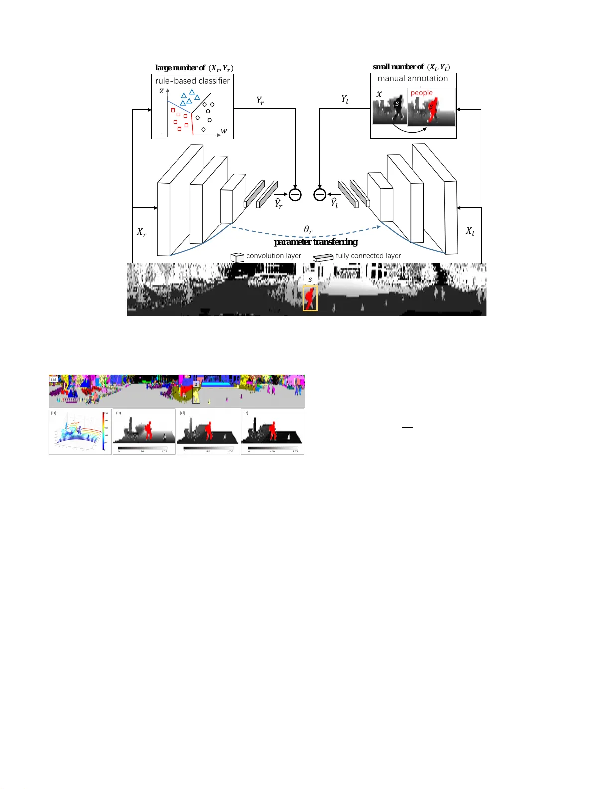
1 Incorporating Human Domain Kno wledge in 3D LiD AR-based Semantic Se gmentation Jilin Mei, Member , IEEE, Huijing Zhao, Member , IEEE Abstract —This work studies semantic segmentation using 3D LiD AR data. Popular deep lear ning methods applied for this task r equire a large number of manual annotations to train the parameters. W e propose a new method that makes full use of the advantages of traditional methods and deep learning methods via incorporating human domain knowledge into the neural network model to reduce the demand f or large numbers of manual annotations and improve the training efficiency . W e first pretrain a model with autogenerated samples from a rule-based classifier so that human knowledge can be propagated into the network. Based on the pretrained model, only a small set of annotations is requir ed for further fine-tuning . Quantitative experiments show that the pretrained model achieves better performance than random initialization in almost all cases; furthermore, our method can achie ve similar perf ormance with fewer manual annotations. Index T erms —3D LiD AR data, semantic segmentation, human domain knowledge. I . I N T RO D U C T I O N Recently , 3D LiD AR sensors ha ve been widely implemented as the “eyes” of autonomous driving systems [1]. Ho w to achiev e ef ficient scene parsing, e.g., semantic segmentation, based on 3D LID AR data has attracted increasing attention. Generally , semantic segmentation is the procedure of finding an object label for each point or data cluster [2]. In this work, the problem is defined as classification based on segmentation, as shown in Fig. 1. Ra w 3D LiDAR data can be equally represented by a range image (b) in the polar coordinate system, where the pixel value is the range distance. Then, ov ersegmentation is conducted on the range frame (c), and the problem of semantic segmentation is solv ed by discriminating the label of each segment (d). 3D LiDAR-based semantic segmentation has been studied for the past decade [2]–[4]. The traditional methods use handcrafted features [3] that hav e a clear definition in the real world, e.g., the width is used to distinguish people from cars. Thus, these methods are interpretable. Ho wev er, the adaptability of features for different scenes remains a challenge, and e xpert knowledge is required to adjust the parameters of the classifier . The outstanding performance of deep learning methods in image semantic se gmentation [5] has encouraged researchers to apply these methods to 3D LiD AR data. These data- driv en methods avoid handcrafted features by using abundant annotated data. Ho we ver , the generation of fine annotations, This work is supported by the National Key Research and Development Program of China (2017YFB1002601) and the NSFC Grants (61573027). Correspondence: H. Zhao, zhaohj@cis.pku.edu.cn. (a )     (b ) (c ) (d ) (e )  - d is ta n c e  - v er t i c a l a n gl e  - h o r i z o n t a l a ng l e Fig. 1. The 3D LiD AR-based semantic segmentation. (a) and (b) show the input data in two kinds of formats, i.e., 3D point cloud and 2D range frame. (c) is the result after over -segmentation. (d) and (e) show the semantic segmentation results. especially for 3D LiD AR data, is challenging, and few public datasets are av ailable for 3D LiD AR-based semantic segmen- tation aimed at autonomous driving applications. The two aforementioned types of methods have their o wn advantages and disadvantages. T raditional methods rely on human domain knowledge, while deep learning methods are data dri ven. Is there a way to combine the advantages and make up for the shortcomings? T o the best of the author’ s knowledge, two techniques ha ve been reported in the literature. The first is a semisupervised approach [6] that con verts human prior knowledge into constraint information, such as data associations between frames, and adds the constraint item to the loss function. W e ha ve v erified the effecti veness of this method in our pre vious work [7]. The second is pretraining, e.g., initializing new networks with parameters trained on IMA GENET [8], which is widely used in tasks related to image processing. The effecti veness of pretraining is discussed in detail in [9]. Howe ver , it is unreasonable to initialize the network parameters directly from an image processing task, which moti vates us to design a pretraining method suitable for 3D LiD AR data. In this paper , we make full use of the advantages of tradi- tional methods and neural network methods via incorporating human domain knowledge into the neural network model to reduce the demand for large numbers of manual annotations 2 and improv e the training efficienc y . The proposed method consists of two steps: parameter pretraining and parameter fine-tuning. In first step, a rule-based classifier based on human kno wledge is designed, and samples are fed through the classifier to perform unsupervised classification. Then, these auto-annotated data are used to pretrain a con volutional neural network (CNN) to ensure that the parameters of the CNN fit the human knowledge. In the second step, the parameters in the pretrained CNN are transferred to a ne w network. Because the new CNN is well initialized, only a small number of manual annotations is necessary to update the parameters. W e ev aluate this method on a dynamic campus scene. Quantitativ e experi- ments show that the pretrained method has better performance than random initialization in almost all cases; furthermore, our method achie ves similar performance with fe wer manual annotations. The remainder of this paper is structured as follows. Sect. II discusses related work. The proposed method is presented in Sect. III. Sect. IV shows the implementation details. Sect. V presents the experimental results. Finally , we draw conclusions in Sect. VI. I I . R E L A T E D W O R K S Semantic se gmentation for 3D LiD AR data is not a new topic. W e firstly re view the methods on semantic segmentation, then discuss how to incorporate human kno wledge. A. Semantic Se gmentation A popular method of semantic segmentation is classification of each point or data cluster . W e separate the related literature into traditional methods and deep learning methods. In traditional methods, some researchers assume that each point or data cluster is independent; for example, [10] presents a versatile framework including feature selection, feature extraction and classification. One-frame LiD AR data usually hav e millions of points, so the direct method is time con- suming. Classification based on a segmentation framew ork is proposed in [3], where only the label of a cluster is ev aluated. Some works consider the spatial relationship be- tween elements, e.g., via the Markov random Field (MRF) or conditional random field (CRF). Features are embedded in node potentials, and spatial relationships are encoded in edge potentials [2]. The solution of a CRF or MRF sometimes requires high-dimensional optimization. Thus, [11] proposes a simplified MRF , where the node and edge potentials are directly updated, and [12] attempts to simplify the point clouds via v oxel-neighbor structure. The main disadv antage of traditional methods is the adaptability of handcrafted features to different scenes. In deep learning methods, features are automatically learned from data. Researchers focus mainly on discussing data rep- resentations and new network structures. Inspired by image semantic segmentation, raw 3D data can be con verted into 2D images. [13] uses virtual 2D RGB images obtaine via Katz projection, and [4], [14] unwrap 3D LiD AR data on spherical range image. Another stream of research considers 3D representations. V oxel occupancy grid is a good way to make irregular raw LiD AR data grid-aligned [15]. The vox el representation is further improved in OctNet [16], which has more efficient memory allocation and computation. New network structures specified for 3D data are also studied. PointNet [17] directly takes raw point clouds as input, and a novel type of neural network is designed with multilayer perceptrons (MLPs). Based on [17], [18] extends the method to incorporate larger-scale spatial context, and [19] proposes the superpoint graph to capture the contextual relationships from point clouds. The main shortcoming of deep learning methods is the demand for large amounts of manual annotations. B. Incorporating Human Knowledge The purpose of incorporating human knowledge is to reduce the need for large numbers of manual annotations in deep learning methods. T o the best of the author’ s knowledge, two types of methods hav e been reported in the literature: semi/weakly-supervised learning and model pretraining. Semi/weakly-supervised learning in volves introducing a fe w fine annotations or large numbers of ambiguous annotations during parameter learning. [20] uses point supervision, where annotators are asked to point to an object if one exists. Then, the point annotation and objectness prior are incorporated into the loss function to train the neural network. Similar work is proposed in ScribbleSup [21], which trains conv olutional networks for semantic segmentation supervised by scribbles. The size constraint of an object is considered in [22]. Our previous work on semisupervised learning implements a pair- wise constraint, which encourages associated samples to be assigned the same labels [7]. Some works focus on training models in weakly supervised settings, such as image-level tags [23], bounding box labels [24] and unlabeled e xamples [25]; these weak supervision methods can be applied separately or in combination. During model pretraining, the tar get network is initialized with the parameters from a pretrained baseline network, e.g., the parameters in the first n layers copy from the baseline network and the remaining parameters are set randomly . This strategy has been widely used in image processing tasks, e.g., segmentation [26] and transfer learning [27]. The baseline net- work is usually trained with IMA GENET [8]. The experiments in [9] confirm and clarify the advantages of unsupervised pretraining, which provides a good initial marginal distribution and exhibits properties of a regularizer . [28] introduces human priors by pretraining a model to regress a cost function under the framework of in verse reinforcement learning. Inspired by [28], we propose a pretraining method suitable for 3D LiD AR data in which large numbers of auto-annotated data are generated with human domain kno wledge. I I I . M E T H O D O L O G Y A. Problem Definition Let P be the range frame con verted from raw 3D point clouds. Segments { s i } N i =1 are obtained on P by e valuating the similarity of 3D points with their neighborhoods, e.g., a region growing method. W e assume that one segment s measures only a single object after ov ersegmentation. As s commonly 3  s m al l n u m be r of (   ,   ) r ul e - ba s ed c l a s s i f i er    ma nu a l a nno t a t i o n peo ple         �   �   l ar ge n u m be r of (   ,   ) para m e te r tran sf e rri n g   c o n v o lu t io n la y er fu lly c o n n ec t ed la y er   Fig. 2. The framework of incorporating human knowledge for 3D LiD AR-based semantic segmentation. The left part is pretraining step and the right is fine-tuning. Fig. 3. The procedure of sample generation from segment. (a) the segment s is chosen as candidate region. (b) the neighbor points around s are cropped to make one sample which has three channels. (c) the range channel, and we mark s with red for better visualization. (d) the height channel. (e) the intensity channel. Please refer to [7] for details. represents a part of the object, a data sample x , including s and the surrounding data, is defined at the center of s , as sho wn in Fig.2. In one range frame P , { s i } N i =1 and { x i } N i =1 can be equally con verted into each other . The problem in this work is formulated as learning a multiclass classifier f θ that maps x to a label y ∈ { 1 , ..., K } and subsequently associates y with the 3D points of s . f θ : x → y ∈ { 1 , ..., K } (1) Giv en a set of annotated data X = { x i } M i =1 , Y = { y i } M i =1 , where { y i } is a one-hot label for { x i } , a common way of learning a classifier f θ is to find the best θ ∗ that minimizes a loss function L , i.e., the cross entropy , as belo w . θ ∗ = arg min θ L ( θ ; X , Y ) L ( θ ; X , Y ) = − 1 M M X i =1 K X k =1 1 [ y k i = 1] ln ( P k θ ( x i )) , (2) where 1 [ ∗ ] is an indicator function and P k θ ( x i ) is the probabil- ity that x i is assigned a label k by a classifier with parameters θ . Stochastic gradient descent (SGD) is commonly applied to solve θ ∗ . Thus, Equation (2) can be re written as: θ ∗ = arg min θ L ( θ ; X , Y , θ 0 ) , (3) where θ 0 is the start position of SGD. θ 0 can be obtained from a random distrib ution, e.g., a truncated normal distribution; or initialized from human knowledge via pretraining, such as in the proposed method. B. W ork Flow As shown in Fig. 2, the framework consists of two steps: parameter pretraining and parameter fine-tuning. One range frame is divided into multiple segments, and each segment corresponds to one sample x in Fig. 3. Consequently , we can automatically produce a large number of samples. The sample generation follows that of [7]. During the pretraining step, we design a rule-based classifier that incorporates human knowledge. The unlabeled samples X r are passed through this classifier to predict the label; thus, the auto-annotated data ( X r , Y r ) are obtained. The rule-based classifier works in an unsupervised manner, and we need not 4 Fig. 4. The definition of features for rule-based classifier . The height z i and width feature w i of segment s i are evaluated. train the classifier via manual annotations. Combining X r and Y r , a CNN is pretrained with a random initialization θ 0 , and the parameters are updated via back-propagation. θ r = arg min θ L ( θ ; X r , Y r , b Y r , θ 0 ) , (4) where b Y r is the output of the CNN. In this way , we obtain the pretrained parameter θ r . b Y r will continue to fit Y r , so we assume that the human rules can be propagated into the CNN. In the fine-tuning step, the pretrained parameters θ r are first transferred into a new neural network. Since the new classifier is well initialized, we need only a small number of manual annotations ( X l , Y l ) for parameter fine-tuning. The parameter updating is the same as in the first step, except that the start position of the optimization is different. The final classifier is obtained by: θ ∗ = arg min θ L ( θ ; X l , Y l , b Y l , θ r ) , (5) where b Y l is the output of the CNN and θ r is the start position. C. Rule-based Classifier LiD AR can directly measure distance information without being affected by illumination, and this rob ust attribute moti- vates us design a classifier based on rules in the real w orld. The sample and segment are associated as detailed in III-A; thus, only features of the segment are considered for each sample in the rule-based classifier . As shown in Fig. 4, the height and width of a segment are calculated from the raw point cloud, and these two features reflect the physical attributes of objects in the real world, i.g., the height of a car generally does not exceed 2 m. W e believe that the width and height of objects are efficient information to design a simple classifier . As shown in Algorithm 1, a trunk is higher than 2 m and has a width in (0, 2.5], people are shorter than 2 m but hav e widths larger than 0.2 m, a car is shorter than 2 m and has a width in [1.5,2.5], and so on. These rules can easily be understood by a human, ho wever , if we want the CNN to understand these rules, the general approach is to train the CNN with a large number of manual annotations. The proposed rule- based classifier can automatically generate annotations without human effort, which accelerates the CNN learning. Algorithm 1 Rule-based Classifier Input: all se gments S in one range frame Output: labeling results Φ 1: Initialize Φ with ∅ 2: for all s i in S do 3: label = U nk now n 4: calculate the width w i and height z i of s i 5: if w i ∈ [0,2.5] and z i > 2 . 0 then 6: label = T r unk  T runk is slim and high 7: else if w i ∈ [0,1.5] then 8: if w i > 0 . 2 then 9: label = P eopl e  People is shorter than 2m 10: end if 11: else if w i ∈ [1.5,2.5] then 12: if z i < 2 . 0 then 13: label = C ar  Car is wider than People 14: end if 15: else if w i ∈ [8.0,15] then 16: label = B uilding  Building is flat 17: end if 18: Φ ← < s i , label > 19: end f or D. P arameter Pr etraining Parameter pretraining has been widely used in image pro- cessing tasks such as classification, detection and segmen- tation, but it is unreasonable to initialize a network toward LiD AR data using the parameters from image processing tasks, as these two types of data are substantially different in terms of both human visual and physical meaning. Therefore, a pre- training approach should be designed for LiDAR data. No w , the question is why pretraining reduces the need for manual annotations during the training phase of neural networks? W e answer the question from two perspectives. Perspecti ve of probability . Human knowledge describes the distribution of the input data X , i.e., P ( X ) , which represents data priors, and the target CNN classifier can be treated as a conditional probability that predicts the label Y for each input data, i.e., P ( Y | X ) . In general, the CNN is trained with only human annotations that are similar to the joint distribution P ( X, Y ) , b ut data priors P ( X ) are ignored. Based on Bayes rule, P ( Y | X ) = P ( Y , X ) /P ( X ) , if accurate priors are supported, we believe that the dependence on manual annotation can be reduced. W e design a rule-based classifier to obtain P ( X ) from human domain kno wledge. Perspecti ve of gradient descent. Gradient descent is the con ventional parameter updating method of CNNs. The selec- tion of the initial position largely determines whether gradi- ent descent can conv erge to the global minimum. Random initialization is a common strategy . The initial position is randomly selected in the high-dimensional parameter space, which increases the possibility of training results falling into local minima. In our method, the samples used for pretraining are supervised by human rules, that is, autogenerated from the rule-based classifier . Thus, the network will continue to fit these rules, and the performance of the pretraining network is related to the rule-based classifier . Although we cannot assume 5 T ABLE I T H E S A MP L E S O F MA N UA L A N N OTA T I O NS . people car trunk bush b uilding cyclist unknown training set 1533 6014 1837 9064 7736 366 5113 testing set 1880 5074 1746 9102 3230 562 4630 T ABLE II T H E P E RF O R M AN C E O F RU L E - B AS E D C L A SS I FI E R . people car trunk building unknown labeling on training set 3009 6255 5914 3596 9723 F1 score on testing set 50.0 64.8 48.9 62.6 66.0 s t ar t V el ody ne G PS/ I MU t he r o u t e f o r t r a ining d a t a t h e r ou t e f or t e s t i n g d a t a Fig. 5. The routes of data collection and the platform configuration. that the pretrained parameters are optimal, they are reasonable. When the initial position of gradient descent starts from the pretrained parameters, the dependence on manual annotation is reduced. In our method, the samples for pretraining are autogenerated by the rule-based classifier , and we do not require any human annotation in this step. E. P arameter F ine-tuning W e define parameter fine-tuning as initializing a new net- work with pretrained parameters and training the network with manual annotations. The main body of a CNN con- sists of con volutional layers and fully connected (FC) layers. Generally , there are two ways to perform parameter fine- tuning in the context of a CNN. Both of them copy the parameters of con volutional layers from a pretrained network to the new network and randomly set the FC layers. The difference is whether the paramters in th conv olutional layers are fixed during fine-tuning. W e test these two configurations in experiments. I V . I M P L E M E N T A T I O N D E TA I L S The CNN used here consists of three conv olutional layers whose dimensions in [width,height,depth] are [256,256,32], [128,128,32], and [64,64,64]; two fully connected layers whose dimensions are both [128,1]; and one softmax layer . In parameter fine-tuning, the CNN predicts 7 labels: people, car , trunk, bush, building, cyclist and unkno wn. In pretraining, the CNN predicts only 5 labels, namely , people, car, trunk, 1440 3420 1640 1680 7933 352 0 1 87 1481 707 227 9 563 9 3 173 57 2118 1143 363 2737 0 0 0 0 1408 3583 2105 1610 8095 228 6 28 210 1250 503 223 79 37 6 17 365 34 125 112 1351 1450 937 2461 1 p e op l e c a r b u il d i n g tr un k un k n ow n p e op l e c a r b u il d i n g tr un k un k n ow n Fig. 6. The comparison between rule-based and CNN-pretrained classifier . The color is indexed by recall, and a darker color means a higher recall. (a) The confusion matrix of rule-based classifier . (b) The confusion matrix of CNN-pretrained classifier . building and unknown since the rule-based classifier cannot fully discriminates cyclist and bush. All networks are trained under the T ensorFlow framework using AD AM solver and a learning rate of 1e-4. The batch size is 2, and we save a checkpoint every 100 iterations. The training phase stops when the loss con verges or is less than 1e-4. For each classifier , we ev aluate all checkpoints on the testing set and select the checkpoint with the highest F1 score. V . E X P E R I M E N T A L R E S U L T S A. Data Set The performance of the proposed method is e valuated on a dynamic campus dataset collected by an instrumented vehicle with a GPS/IMU suite and a V elodyne-HDL32, as sho wn in Fig. 7. The total route is approximately 890 meters. All sensor data are collected, and each data frame is associated with a time log for synchronization. The GPS/IMU data are logged at 100 Hz. The LiD AR data are recorded at 10 Hz and include 1039 frames of training data (red line in Fig. 5) and 790 frames of testing data (black line in Fig. 5). One frame can produce multiple samples; for example, we obtain 6014 car samples from the 1039 frames of training data in T ABLE I. T o make quantitativ e comparisons, manual annotations [7] are conducted on both training and testing sets; the labeling results are shown in T ABLE I. 6 T ABLE III T H E C O MPA R IS O N S W I T H F 1 M E A S UR E ON T ES T I N G S E T . classifier people car trunk building unknown mean score rule-based 50.0 64.8 48.9 62.6 66.0 58.5 pretrained-CNN 57.4 67.0 50.4 66.0 67.2 61.6 T ABLE IV T H E S U BD I V I SI O N O F T RA I N IN G S ET F OR F UN E T U NI N G . finetuning data people car trunk bush building cyclist unkno wn training set 1533 6014 1837 9064 7736 366 5113 sub-100 100 100 100 100 100 100 100 sub-400 400 400 400 400 400 366 400 sub-1600 1533 1600 1600 1600 1600 366 1600 T ABLE V T H E F 1 S C O RE O F D I FF ER E N T C L A SS I FI E RS O N T E ST I N G S E T . finetuning data classifier people car trunk bush building cyclist unknown mean score sub-100 baseline-100 46.0 56.5 66.3 65.5 56.0 30.8 35.8 51.0 pretrain-100 55.0 71.6 68.6 63.9 61.8 31.3 39.4 55.9 sub-400 baseline-400 59.4 72.2 73.5 71.4 71.8 44.0 35.1 61.1 pretrain-400 67.1 79.7 71.9 72.8 70.8 45.5 48.5 65.2 sub-1600 baseline-1600 68.7 80.3 74.4 70.8 69.9 46.1 48.9 65.6 pretrain-1600 71.2 82.5 75.9 75.9 72.6 46.5 49.0 67.7 training set baseline-all 69.2 85.1 77.2 75.3 76.8 44.6 53.8 68.8 pretrain-all 71.6 87.5 80.2 77.1 78.2 45.4 53.6 70.5 1 baseline-* : random initialization; pretrain-* : pretraining initialization(ours). B. Rule-based Classifier The rule-based classifier is simple, and its effecti veness should be assessed before conducting further experiments. As shown in T ABLE. II, we pass both training and testing sets through this classifier which assigns one label for each sample. Currently , the classifier supports only 5 categories. In this way , we collect the auto-annotated training set (the second row of T ABLE. II) for parameter pretraining. At the same time, the effecti veness is ev aluated on the testing set in the term of F1 measure, which is defined as: F 1 − M easur e = 2 ∗ r ecall ∗ precision r ecall + precision · 100 . (6) W e mer ge bush and c yclist in T ABLE. I into unkno wn when calculating the F1 score for the rule-based classifier, and the results are shown in the third ro w of T ABLE. II. The F1 scores in T ABLE. II are encouraging: simple rules ensure reasonable results, and the rule-based classifier is effecti ve. The confusion matrix is shown in Fig. 6 (a), one notable result is that the recall of trunk is very high. C. Pretr aining Results The CNN is trained with the autolabeled samples in T ABLE. II. W e expect the pretrained CNN to have similar performance 0.25 0.35 0.45 0.55 0.65 0.75 0.85 0.95 people car trunk bush building cyclist unknown F1 measure B-100 B-400 B-1600 B -all P-100 P-400 P-1600 P- all x100 Fig. 7. The quantitative comparison of different classifiers. B-* means baseline and P-* means pretrained classifier . to the rule-based classifier since the samples are supervised by the rules. As illustrated in T ABLE. III, the pretrained CNN has better F1 scores on each category than does the rule-based method. A more detailed comparison is in Fig. 6. These two classifier has very similar performances, i.g., they both achieve high recalls on trunk. On the basis of these results, we assume that the rules designed by humans have propagated into the pretrained CNN and that the parameters of CNN are more 7 reasonable than random initialization. W e emphasize that pretraining dose not require any man- ual labeling. Although the samples are supervised by rules, the pretrained CNN still performs better than the rule-based classifier . D. Fine-tuning Results The fine-tuning data has four components as shown in T ABLE. IV. Sub-100 ∼ 1600 are randomly selected from the raw training set. F or example, sub-1600 means choosing 1600 samples from each cate gory . If the number of sample is less than 1600, such as for people and c yclist categories, we do not perform any sample augmentation. As illustrated in T ABLE. V and Fig. 7, different classifiers are tested based on the fine-tuning data. Baseline-* means the parameters are initialized with the truncated normal distribu- tion, and pretrain-* means the parameters in the con volutional layers copy from the pretrained network. All classifiers share the same network structure detailed in Sect. IV. First, we discuss the results of a few annotations. our method performs better than the random v ersion under sub- 100 and sub-400; furthermore, the mean score of pretrain-400 is near that of baseline-1600, which illustrates the potential of our method to achieve high performance fewer manual annotations. Second, from the perspecti ve of category scores, the highest scores belong mostly to the classifiers initialized by human rules. Third, from the perspecti ve of mean scores as shown in Fig. 8, the pretrained versions ha ve higher scores than the random versions under the same manual annotations: pretrain-400 is near baseline-1600, and pretrain-1600 is near baseline-all. Another notable result is that the gap between random and pretrained initialization becomes small as the number of manual annotations increases. In conclusion, human rules help to reduce the demand for manual annotations. T wo methods of parameter fine-tuning are discussed in Sect. III-E. Pretrain-* in Fig. 8 indicates the first way , where the parameters of conv olutional layers are updated during fine- tuning, and the pretrain-fix-* indicates that the conv olutional parameters are initialized from the pretrained network and are fixed during fine-tuning. W e find that the F1 scores of pretrain- fix-100 are higher than those of pretrain-100, b ut as the manual annotations increases, the performance of pretrain-fix trends to become stable, e.g., pretrain-fix-1600 and pretrain-fix-all have almost the same score. These results sho ws that the fixed fine- tuning method has better adaptability for cases with very few annotations. V I . C O N C L U S I O N A N D F U T U R E W O R K In this paper , we propose a new method aimed at seman- tic segmentation based on 3D LiD AR data. T o reduce the substantial demand for manual annotations during parameter training, we attempt to incorporate human knowledge into a neural netw ork via parameter pretraining. T o this end, we first pretrain a model with the autogenerated samples from a rule- based classifier so that human kno wledge can be propagated into the netw ork. Based on the pretrained model, only a small set of annotations are required to perform further finetuning. 0.45 0.5 0.55 0.6 0.65 0.7 0.75 100 400 1600 all baseline pretrain pre train-fix x100 F1 measure Fig. 8. The mean F1 scores of dif ferent classifiers. This method is examined extensi vely on a dynamic scene. The promising results indicate reduced reliance of manual annotation. Future work will consider the addition of more priors/knowledge, e.g., the spatial and temporal relationships between samples. R E F E R E N C E S [1] C. Urmson, J. Anhalt, D. Bagnell, C. Baker , R. Bittner, M. Clark, J. Dolan, D. Duggins, T . Galatali, C. Geyer et al. , “ Autonomous dri ving in urban en vironments: Boss and the urban challenge, ” Journal of Field Robotics , vol. 25, no. 8, pp. 425–466, 2008. [2] D. Munoz, N. V andapel, and M. Hebert, “Onboard contextual classifica- tion of 3-d point clouds with learned high-order markov random fields, ” in IEEE International Conference on Robotics and A utomation . IEEE, 2009, pp. 2009–2016. [3] H. Zhao, Y . Liu, X. Zhu, Y . Zhao, and H. Zha, “Scene understanding in a large dynamic environment through a laser-based sensing, ” in IEEE International Confer ence on Robotics and Automation . IEEE, 2010, pp. 127–133. [4] G. L. O. a. B. A yush Dewan, “Deep semantic classification for 3d lidar data, ” in IEEE/RSJ International Conference on Intelligent Robots and Systems . IEEE, 2017, pp. 3544–3549. [5] A. Garcia-Garcia, S. Orts-Escolano, S. Oprea, V . V illena-Martinez, and J. Garcia-Rodriguez, “ A review on deep learning techniques applied to semantic segmentation, ” arXiv pr eprint arXiv:1704.06857 , 2017. [6] R. Y an, J. Zhang, J. Y ang, and A. G. Hauptmann, “ A discriminati ve learning framework with pairwise constraints for video object classifica- tion, ” IEEE T ransactions on P attern Analysis and Machine Intelligence , vol. 28, no. 4, pp. 578–593, 2006. [7] J. Mei, B. Gao, D. Xu, W . Y ao, X. Zhao, and H. Zhao, “Semantic segmentation of 3d lidar data in dynamic scene using semi-supervised learning, ” arXiv pr eprint arXiv:1809.00426 , 2018. [8] O. Russakovsk y , J. Deng, H. Su, J. Krause, S. Satheesh, S. Ma, Z. Huang, A. Karpathy , A. Khosla, M. Bernstein, A. C. Berg, and L. Fei-Fei, “ImageNet Large Scale V isual Recognition Challenge, ” International Journal of Computer V ision (IJCV) , vol. 115, no. 3, pp. 211–252, 2015. [9] D. Erhan, Y . Bengio, A. Courville, P .-A. Manzagol, P . V incent, and S. Bengio, “Why does unsupervised pre-training help deep learning?” Journal of Machine Learning Resear ch , v ol. 11, pp. 625–660, 02 2010. [10] M. W einmann, B. Jutzi, and C. Mallet, “Semantic 3d scene interpreta- tion: A framework combining optimal neighborhood size selection with relev ant features, ” ISPRS Annals of Photogrammetry , Remote Sensing and Spatial Information Sciences , vol. II-3, pp. 181–188, 2014. [11] Y . Lu and C. Rasmussen, “Simplified mark ov random fields for ef ficient semantic labeling of 3d point clouds, ” in IEEE/RSJ International Con- fer ence on Intelligent Robots and Systems . IEEE, 2012, pp. 2690–2697. [12] T . W ang, J. Li, and X. An, “ An efficient scene semantic labeling approach for 3d point cloud, ” in IEEE International Conference on Intelligent T ransportation Systems . IEEE, 2015, pp. 2115–2120. [13] P . T osteberg, “Semantic se gmentation of point clouds using deep learn- ing, ” Master’s thesis, Link ¨ oping University , 2017. [14] B. W u, A. W an, X. Y ue, and K. Keutzer , “Squeezeseg: Conv olutional neural nets with recurrent crf for real-time road-object segmentation from 3d lidar point cloud, ” arXiv pr eprint arXiv:1710.07368 , 2017. 8 [15] T . Hackel, N. Savinov , L. Ladicky , J. D. W egner, K. Schindler, and M. Pollefeys, “SEMANTIC3D.NET: A new large-scale point cloud classification benchmark, ” ISPRS Annals of the Photogrammetry , Remote Sensing and Spatial Information Sciences , vol. IV -1-W1, pp. 91–98, 2017. [16] G. Riegler , A. O. Ulusoy , and A. Geiger, “Octnet: Learning deep 3d representations at high resolutions, ” in IEEE Confer ence on Computer V ision and P attern Reco gnition , vol. 3. IEEE, 2017, pp. 6620–6629. [17] C. R. Qi, H. Su, K. Mo, and L. J. Guibas, “Pointnet: Deep learning on point sets for 3d classification and segmentation, ” in IEEE Conference on Computer V ision and P attern Recognition . IEEE, 2017, pp. 77–85. [18] F . Engelmann, T . Kontogianni, A. Hermans, and B. Leibe, “Exploring spatial context for 3d semantic segmentation of point clouds, ” in IEEE Confer ence on Computer V ision and P attern Reco gnition . IEEE, 2017, pp. 716–724. [19] L. Landrieu and M. Simonovsk y , “Large-scale point cloud semantic segmentation with superpoint graphs, ” arXiv preprint , 2017. [20] A. Bearman, O. Russako vsky , V . Ferrari, and L. Fei-Fei, “Whats the point: Semantic segmentation with point supervision, ” in Eur opean Confer ence on Computer V ision . Springer , 2016, pp. 549–565. [21] D. Lin, J. Dai, J. Jia, K. He, and J. Sun, “Scribblesup: Scribble- supervised con volutional networks for semantic segmentation, ” in IEEE Confer ence on Computer V ision and P attern Reco gnition . IEEE, 2016, pp. 3159–3167. [22] G. Papandreou, L.-C. Chen, K. P . Murphy , and A. L. Y uille, “W eakly-and semi-supervised learning of a deep con volutional network for semantic image segmentation, ” in IEEE International Confer ence on Computer V ision . IEEE, 2015, pp. 1742–1750. [23] D. Pathak, P . Krahenb uhl, and T . Darrell, “Constrained con volutional neural networks for weakly supervised segmentation, ” in IEEE Interna- tional Conference on Computer V ision . IEEE, 2015, pp. 1796–1804. [24] J. Dai, K. He, and J. Sun, “Boxsup: Exploiting bounding boxes to supervise con volutional netw orks for semantic segmentation, ” in IEEE International Confer ence on Computer V ision . IEEE, 2015, pp. 1635– 1643. [25] J. Xu, A. G. Schwing, and R. Urtasun, “Learning to segment under various forms of weak supervision, ” in IEEE Confer ence on Computer V ision and P attern Reco gnition . IEEE, 2015, pp. 3781–3790. [26] J. Long, E. Shelhamer, and T . Darrell, “Fully conv olutional networks for semantic se gmentation, ” in IEEE conference on computer vision and pattern recognition , 2015, pp. 3431–3440. [27] J. Y osinski, J. Clune, Y . Bengio, and H. Lipson, “How transferable are features in deep neural networks?” Advances in Neur al Information Pr ocessing Systems (NIPS) , vol. 27, 2014. [28] M. W ulfmeier , D. Rao, and I. Posner, “Incorporating human domain knowledge into lar ge scale cost function learning, ” arXiv preprint arXiv:1612.04318 , 2016. Jilin Mei received B.S. degree in automation in 2014 from University of Electronic Science and T ech- nology of China, Chengdu, China. He is currently working to ward the Ph.D. de gree in intelligent robots in the Key Lab of Machine Perception (MOE), Peking University , Beijing, China. His research interests include intelligent v ehicles, computer vision and machine learning. Huijing Zhao received B.S. degree in computer science in 1991 from Peking Univ ersity , China. From 1991 to 1994, she was recruited by Peking Univ ersity in a project of developing a GIS platform. She obtained M.E. degree in 1996 and Ph.D. de gree in 1999 in civil engineering from the University of T okyo, Japan. After post-doctoral research as the same university , in 2003, she was promoted to be a visiting associate professor in Center for Spatial Information Science, the University of T okyo, Japan. In 2007, she joined Peking Uni v as an associate professor at the School of Electronics Engineering and Computer Science. Her research interest covers intelligent vehicle, machine perception and mobile robot.