GlidarCo: gait recognition by 3D skeleton estimation and biometric feature correction of flash lidar data

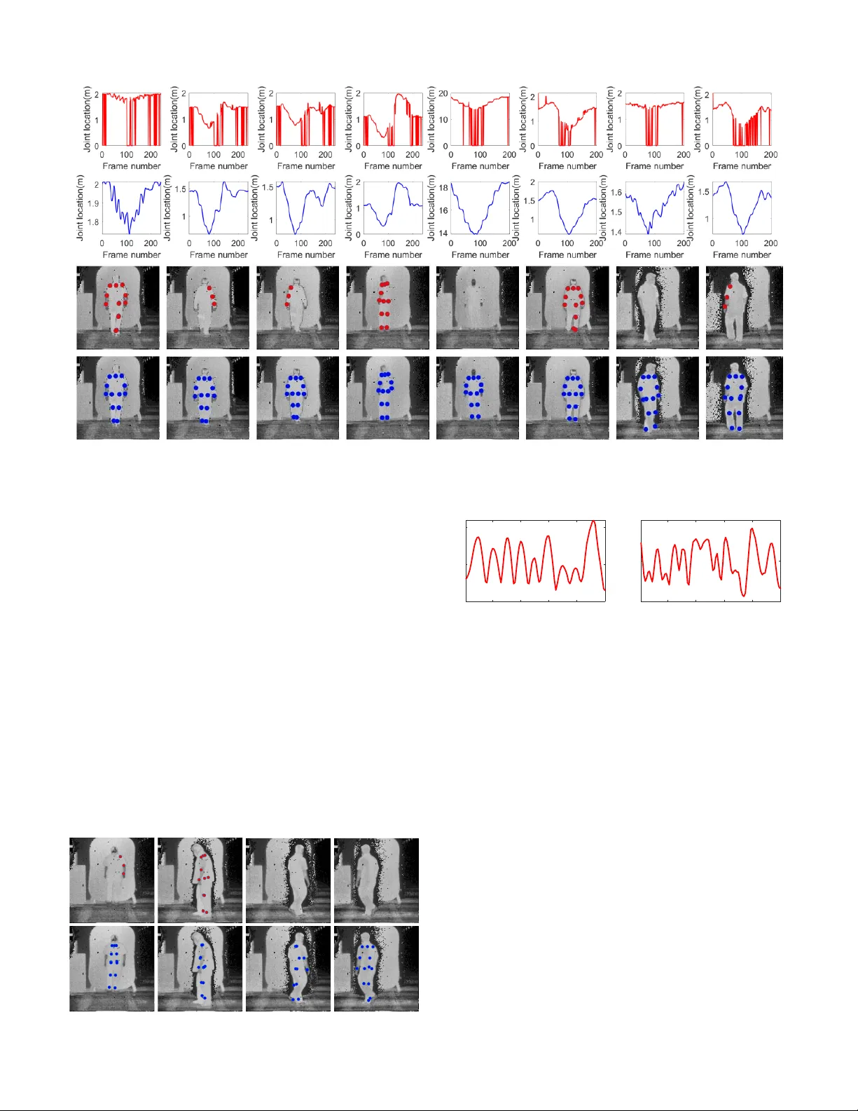
1 GlidarCo: gait recognition by 3D sk eleton estimation and biometric feature correction of flash lidar data Nasrin Sadeghzadehyazdi, T amal Batabyal, Nibir K. Dhar , B. O. Familoni, K. M. Iftekharuddin, Scott T . Acton Abstract —Gait r ecognition using nonin vasiv ely acquired data has been attracting an increasing inter est in the last decade. Among various modalities of data sources, it is experimen- tally found that the data in v olving skeletal repr esentation are amenable for r eliable feature compaction and fast processing. Model-based gait recognition methods that exploit featur es from a fitted model, like skeleton, are recognized f or their view and scale-in variant properties. W e propose a model-based gait recog- nition method, using sequences r ecorded by a single flash lidar . Existing state-of-the-art model-based approaches that exploit features from high quality skeletal data collected by Kinect and Mocap are limited to controlled laboratory en vironments. The performance of con ventional research efforts is negatively affected by poor data quality . W e address the problem of gait recognition under challenging scenarios, such as lower quality and noisy imaging process of lidar , that degrades the perfor - mance of state-of-the-art skeleton-based systems. W e present GlidarCo to attain high accuracy on gait recognition under the described conditions. A filtering mechanism corrects faulty skeleton joint measurements, and rob ust statistics are integrated to conv entional feature moments to encode the dynamic of the motion. As a comparison, length-based and vector -based features extracted from the noisy skeletons are inv estigated for outlier r emoval. Experimental r esults illustrate the efficacy of the proposed methodology in improving gait recognition given noisy low resolution lidar data. Index T erms —gait recognition, lidar , feature correction, outlier detection I . I N T R O D U C T I O N G AIT identification has recei ved an increasing interest in the last decade due to the v arious applications in areas ranging from intelligent security surveillance and iden- tifying person of interest in criminal cases, to designated smart en vironments [1], [2]. Besides, gait analysis plays an Nasrin Sadeghzadehyazdi, T amal Batabyal, and Scott T . Acton are with the Charles L. Bro wn Department of Electrical and Computer Engineer - ing, University of Vir ginia, Charlottesville, V A 22904-4743, USA (e-mails: ns8va@vir ginia.edu, tb2ea@virginia.edu and acton@virginia.edu.) Nibir K. Dhar, and B. O. Familoni are with Night V ision and Electronic Sensors Directorate Fort Belvoir , USA K. M. Iftekharuddin is with department of electrical and computer engi- neering, Old Dominion Univ ersity , 231 Kaufman Hall Norfolk, V A 23529, USA (e-mail: kiftekha@odu.edu.) Distribution Statement A: Approv ed for public release. Distribution is unlimited IEEE Copyright Notice: c  IEEE 2019 Personal use of this material is permitted. Permission from IEEE must be obtained for all other uses, in any current or future media, including reprinting/republishing this material for advertising or promotional purposes, creating new collective works, for resale or redistribution to servers or lists, or reuse of any copyrighted component of this work in other works. Fig. 1: Sample frames of lidar data. The top and bottom rows show range and intensity data, respectively . important role to quantify the se verity of certain motion-related diseases like Parkinson [3]. Gait recognition aims to tackle the identification problem based on the way people walk and early studies findings in the medical and psychology hav e shown the uniqueness of gait to individuals [4], [5]. While the iris [6], face [7], [8], and fingerprint [9] provide some of the most efficacious biometrics for person identification with high recognition accuracy , they require the cooperation of subjects as well as av ailability of high quality data. In real life howe ver , there are man y scenarios in which the subjects cannot be controlled, there is no contact between subjects and sensors, or access to the high quality data is not possible. Under such circumstances, biometrics that can be extracted from the gait hav e shown promising results in several studies [10], [11], [12]. Features extracted from gait are resilient to changes in clothing or lighting conditions compared to color or texture which are among pre valent features for person identification. While patterns of walking may not be necessarily unique to individuals in practice, a combination of biometric-based static attributes along with the motion analysis of certain joints can create an ef fectiv e set of features to recognize one individual from another . In recent years, depth cameras hav e become popular for gait analysis mainly due to their ability to provide a three di- mensional depiction of the scene [13], [14], [15]. Unlike their optical counterparts, depth cameras like lidar and Kinect can provide depth information that is not sensitiv e to illumination and changing in the lighting conditions that are among major issues in uncontrolled en vironments. This makes depth camera an ideal candidate for long-term person identification that rely on features such as time-in variant biometrics. In this work, we utilize the flash lidar technology to collect data. A flash lidar 2 camera uses pulsed laser to illuminate the whole scene and simultaneously record range (depth) and intensity information. Figure 1 shows sample frames of the collected intensity and range data by the flash lidar camera. Since the laser beams can be focused to suit the objects of interest, a flash lidar camera can provide detailed depth imaging of the scene. This property of flash lidar has lead to extensiv e applications in areas such as autonomous vehicles, atmospheric physics, archaeology , forestry , geology , geography , seismology , space missions, and transportation. V ideo-based gait recognition approaches are generally di- vided into two main categories, model-based, and model-free methods. Model-free methods rely on features that can be obtained from clean silhouettes [16], [17]. They are easy to im- plement and computationally less expensi ve compared to their model-based counterparts. Howe ver , model-free methods are not view and scale in variant, and require recordings from mul- tiple angles that is not always feasible from applicability point of view . Using skeleton for gait recognition is categorized as a model-based approach for person identification. Most of the existing methods rely on fitting a model, usually a skeleton, to human silhouettes [18], [19]. The main issue with the model- based methods is the fact that in general, model fitting is a computationally expensiv e process. While such difficulties are not an issue with structured lighting approaches such as Kinect due to the direct estimation of joints coordinates, the working range of Kinect is limited. Furthermore, the range information of Kinect is not reliable in outdoor environments, because it is not easy to differentiate the infrared light of the sensor from the high intensity infrared of environment [20], [21]. T o curb the computational complexity of model-based methods, sev eral studies rely on high-quality real-time skeleton joints data generated by Mocap [22], [23]. Howe ver , in terms of applicability , Mocap is limited to a laboratory en vironment which is a major drawback. Unlike Mocap, flash lidar has been extensi vely used for outdoor applications. Compared with Kinect, a flash lidar camera has a drastically extended range ( > 1000 meters) and its performance is not de graded in outdoor en vironments due to the high irradiance power of pulsed laser generated by lidar compared with the background [24]. W ith a limited number of studies, the only existing lidar- based person identification works in the literature are model- free and rely on background subtraction to extract human silhouette from the point cloud data provided by V elodynes Rotating Multi-Beam (RMB) lidar system [25], [26], [17]. In this work howe ver , we take a model-based approach, le ver - aging OpenPose, a pre-trained deep network [27] to extract a skeleton model from the intensity information. Using camera properties and the depth data, the provided skeleton joint coordinates are transferred into real-world coordinates. The work presented here can be employed for gait analysis in different applications; for instance to impro ve the classification results by including gait information in our pre vious w ork [28]. This shift of the modality from the structured (image/video) to unstructured (skeleton) data type provides benefits in terms of data compaction, computation, storage, scalability , and recognition accuracy . Furthermore, the skeleton-related at- tributes mimic actual physical traits in human body and can be utilized as a soft biometric ID for the individuals. Our visual system does not extricate details of clothing texture, or the skin tone of the person who is walking. Rather , it focuses on certain body parts (joints, limbs), and tries to reconstruct the anatomy and locomotion. Such biological cues are exploited in [29], [30]. In addition, there has been a surge of studies to find a suitable model for such purpose [31], [32], [33]. Existing successful model-based methods take advantage of high-quality skeleton data provided by Kinect or Mocap and av oid the challenge of erroneous features. Ho wev er , as we mentioned earlier, these modalities are not a proper choice for real-world applications. In contrast with Kinect and Mocap, the data collected by a flash lidar camera is noisy and has low resolution that degrades the performance of sk eleton extraction systems. Features that are computed from the faulty skeleton models are plagued with erroneous measurements that in turn present a major challenge for a successful gait recognition. In this paper , our main goal is to answer the following question, ”When the collected data is noisy to a level that a considerable number of fitted skeleton models contain missing or erroneous joints, is it still possible to identify gaits with a high accuracy and precision?”. In particular under the described condition, ”Can we avoid the common approach of removing noisy data, and correct the faulty skeletons, instead?” T o address these questions, we present GlidarCo, a methodology to correct for the faulty and missing measurements of joint coordinates, and integrate the robust statistics to improve gait recognition using the noisy , low resolution flash lidar data. Our contributions are fourfold. First, we present a model- based approach for gait recognition using flash lidar data that is close to real-time. Second, we present a filtering mechanism that exploits robust statistics and shape-preserving interpolation to correct for faulty and missing measurements of joint coordinates. Third, we integrate robust statistics with the traditional feature moments to incorporate the motion dynamics over the gait cycles. F ourth, as an alternative method for applications where data elimination is not an issue, we in vestigate features extracted from noisy skeletons for outliers, and present a modification of the T ukey’ s method for vector - based feature vectors. The latter contribution is an effort to follow the traditional practice of removing noisy data and perform classification on the remaining clean data. In particular , we aim to compare the results from outlier removal method, with an unorthodox ef fort that seeks to correct the erroneous data. W e must emphasize the importance of the latter , as it preserves the original data, that is costly to collect in many applications. An extensi ve experimental inv estigation demonstrates the efficacy of the proposed methodology in improving the performance of both length-based and vector- based features for gait identification using the flash lidar data. The rest of this paper is presented as follows. In the next section, we will outline the related work. Next, we will describe the proposed methodology in detail in the Meth- ods section. The results and discussion describes a thorough experimental in vestigation into the efficac y of the proposed method and compares the performance of multiple set of features, including state-of-the-are methods in the context of 3 gait recognition before and after data correction. Finally , we summarize in the conclusion section. I I . R E L ATE D W O R K Model-based methods fit a model, like a skeleton, to human body and use the features extracted from the fitted model to identify g aits. Model fitting is generally a comple x and computationally expensi ve process. T o avoid such difficulties, many studies lev erage Kinect as a marker-less motion capture tool, that generates a real-time high quality intensity and depth data, along with joint information of skeleton. In general, these methods are based on identifying gait cycle and calculating static anthropometric-based features like bone lengths and height, gait features like step length and gait cycle or angle between selected body joints ov er each gait cycle. Statistics like mean, maximum, and standard deviation of the collected attributes are computed ov er each gait cycle and utilized as feature identifiers. Using maximum, mean, and standard de viation of a set of lower body angles over a half gait c ycle as features and K-Means clustering algorithm, Ball et al . [34] acquired an accuracy of 43.6% on a dataset collected from four subjects. In [11], authors used a set of static features plus two gait features and achiev ed an accuracy of 90% on a dataset collected from nine subjects walking from right to left in front of a Kinect camera. Araujo et al . [35] used eleven static anthropometric features and in vestigated the effect of different subset of features in gait recognition. They also compared the performance of four different classifiers on a dataset collected from eight different subjects. An average accurac y of 98% was obtained only when the training and test samples contained the same type of walking pattern. Sinha et al . [12] proposed a set of area-based features plus distance between different body segment centroids and combined these attributes with features in [34] and [11] and obtained a higher accuracy compared with the work of Ball and Preis on a dataset of ten subjects. Kumar and Babu [36] proposed a set of covariance-based measures on the trajectory of skeleton joints, and acquired an accuracy of 90% on a dataset of 20 subjects. Diko vski [37] ev aluates the performance of different features like angles of lower body joints, distance between adjacent joints, height and step length ov er one gait cycle. Relative distance and relati ve angles are computed between selected body joints and compared together utilizing the Dynamic Time W arping (DTW) algorithm by Ahmed et al . [38]. Ali et al . [39] compute triangles formed by lower body joints during motion and utilize mean of the areas during one gait c ycle. In [40] Y ang et al . use a set of anthropometric and relative distance-based features for identification. The majority of previous model-based studies exploit se- quences that were recorded on a limited w alking patterns. Subjects walk on straight lines and training and test sequences include the same patterns of w alking. In this w ork, we consider a case that inv olves different patterns of walking. In particular, we select disparate walking patterns for training and test sequences. This paper is an extension of our previous work [41], with an improvement on joint coordinate filtering and per - Depth data Intensity data 2D Skeleton detector 3D Joint location estimator Feature extraction Joint Correction Person ID Gait Recognition Fig. 2: Pipeline for gait recognition using joint correction criterion of GlidarCo 3D Joint location estimator Person ID Feature extraction Outlier removal Gait recognition Fig. 3: Pipeline for outlier removal. Inputs to ”3D Joint location estimator” remain the same as in Figure 2 frame identification. Furthermore, we propose a new method to integrate the dynamic of the motion. W e also present an outlier remov al method for vector -based feature vectors that can be employed in applications that data remov al is not an issue. In addition, we ev aluate the proposed methodologies on two different feature vectors, and compare with more state-of- the-art relev ant methods. In our dataset, recorded by a single flash lidar camera, sev eral factors diminish the quality of features that are com- puted from the resulting joints. As the subjects proceed tow ard the camera, range data are af fected by noise. The lack of color in the intensity data, and similarity between human clothing, background and skin are some of the other elements that can negati vely af fect the quality of detected poses and consequently the feature vectors. A common approach in the existing studies in volv es the removal of outlier noisy data that are generated as a result of faulty measurements. Further processing is applied on the remaining higher quality collection of joint data. In this paper , we propose an automated outlier remov al procedure. Howe ver , with the shortage of data being a major challenge in many real-world surveillance scenarios, data remov al will only exacerbate the data scarcity problem. In other words, while outlier removal can be a proper solution to gather higher quality data to begin with, it is not the best choice when data elimination can raise issues. W e aim Fig. 4: T op row: sample frames with correctly detected skeletons, bottom row: frames with faulty skeletons 4 to address this problem by proposing a filtering mechanism that corrects erroneous joint data, instead of eradicating them. Figure 2 and 3 present the pipeline of joint correction and outlier removal methodologies, respectiv ely . T o prove the efficacy of the proposed methodology , we will compare the performance of two different sets of features, length-based and vector -based features, and four state-of-the- art works, before and after joint correction. Furthermore, as an alternativ e for applications in which data elimination is not an issue, we also consider automatic outlier removal and compare it with the proposed joint correction on impro ving the gait identification accuracy . I I I . M E T H O D S A. Overview of method Figure 2 describes the workflo w of the proposed gait recognition methodology using flash lidar data. F or a lidar sequence V with f frames, there exists I = [ I 1 , I 2 , ..., I f ] , and R = [ R 1 , R 2 , ..., R f ] , where I i and R i represent intensity and range data at frame i . Images are preprocessed to reduce noise and are fed into a 2D skeleton detector . W e leverage OpenPose a state-of-the-art real-time pose detector to fit a skeleton model and extract the location of body joints. In Figure 4, the top row sho ws examples of correctly detected skeleton joints. As we can see in this figure, OpenPose provides a skeleton model of 18 joints, where 5 of the joints represent nose, eyes, and ears. Howe ver , the model that we adopt in this paper only considers 13 joints. The reason for such choice is the fact that face joints are missing from a large majority of our samples. Furthermore, the facial joints do not conv ey useful information for gait recognition. Figure 5 illustrates the skeleton model that we use in this work. Given I i as the input to the skeleton detector , the output is the joint location coordinates that can be represented with the following vectorized form J i = [ x k , y k ] M j k =1 ∈ < 2 N (1) where ( x k , y k ) are the coordinates of the k th joint in the image frame of reference, and M j represents the number of joints. Using the range data and the properties of the lidar camera, we can project the 2-dimensional coordinates of joints into real-world coordinates. L i j , the real-world location of joint i in the direction j can be calculated according to the following equation L i j = 2 N pixels × tan( θ aov 2 ) × Lp i j × D i camera (2) where N pixels is the number of pixels in the j direction, θ aov represents the angle of vie w , and D i camera is the range v alue of joint i . Lp i j represents the location of joint i in the direction j in the image coordinate system. Here j is in the x or y direction, and the L i in the z direction equals to the depth value at the location of the joint i . As we discussed earlier, the quality of the resulting skeleton and the joint localization are negati vely affected by several factors. The features that are computed using the acquired skeletons are plagued with erroneous measurements. There- fore, gait recognition based on the computed faulty skeletons I n d e x Join t 1 M i d S h o u l de r 2 R i g h t S h o ul de r 3 R i g h t E l b o w 4 R i g h t W r i s t 5 L e f t S h o ul d e r 6 L e f t E l b o w 7 L e f t W r i s t 8 R i g h t H i p 9 R i g h t Kn e e 10 R i g h t An k l e 11 L e f t H i p 12 L e f t Kn e e 13 L e f t An k l e Fig. 5: The skeleton model we use in this work. Left: index of each joint in the skeleton model. Right: skeleton model in a sample frame. results into a high rate of false positives. T o resolve this problem, we present a filtering mechanism that employs robust statistics and shape-preserving interpolation to correct for faulty measurements in time sequences of joint coordinates values. This filter will improve the quality of the joint local- ization and ultimately enhance the gait recognition accuracy . As an alternativ e approach for the joint location correction, we employ the T ukey method to detect and remove length-based and vector-based feature vectors. In particular , we present a modification for vector -based outlier detection using the T ukey method. The following subsection giv es the description of the filtering mechanism, which is followed by the outlier remov al subsection. B. F iltering of joint location Let L be a matrix of the size of 39 × F n , where each row represents the time sequence of one joint in one of the direction of x, y , and z , extended ov er F n frames. Since each skeleton consists of 13 joints, there are in total 39 joint coordinate time sequences. In order to correct for missing joint location values and noisy outliers in a giv en video, we perform filtering of joint location on each row of the corresponding L matrix. Let L m represent the m -th row of L L m = [ L m ( t )] F n t =1 L m ( t ) ∈ < (3) Giv en joint location sequence L m , first we use T ukey’ s test to detect any value in L m that is below Qu low − 1 . 5 × I QR , or above Qu up + 1 . 5 × I QR where I QR stands for the interquartile range, Qu low and Qu up are lo wer and upper quartile, respecti vely . If o L m is the set of all the detected outlier indices in L m (each index corresponds with one time instant t ) defined as      o L m = [ o 1 , o 2 , ..., o R ] o 1 < o 2 < ... < o R o i ∈ [1 , 2 , ..., F n ]; i ∈ [1 , 2 , ..., R ] (4) where R is the number of outliers in L m detected by the T ukey’ s method, then L m ( o i ) will be corrected according to 5 the following L c m ( o i ) = L N O m L N O x = 1 − N N ( L m ( o i )) (5) where L c m ( o i ) is the corrected value of L m at t = o i . N O and 1 − N N stand for non-outlier , and the one nearest neighbor , respectiv ely . L N O m is the value of the nearest neighbor of L m ( o i ) , that is not an outlier . In those cases with two nearest neighbors, one is selected randomly . After the detected outlier values of L m are corrected according to equation 5, piece-wise cubic Hermite polynomials [42] are utilized to interpolate the missing values in L m . W e use piece-wise Hermite polynomial to preserve the shape of L m . Meanwhile, by applying outlier correction before missing value interpolation, the shape of the curves will be less affected by outliers. Finally , we employ RLowess (locally weighted scattered plot smoothing) filter [43] to smooth the resulting joint location sequence and alleviate the ef fect of remaining smaller spikes in L m . RLowess assigns a value to each point by locally fitting a first- order polynomial, utilizing weighted least squares. W eights are computed using the median absolute deviation (MAD), which is a robust measure of variability in the data in the presence of outliers. The robustness of weights is critical due to the existence of smaller-amplitude spikes that act as outliers. The described filtering procedure will effecti vely cor- rect joint location time sequences. Furthermore, when pose- detector fails to detect a skeleton model, the joint location filtering can interpolate the missing skeleton joint locations. Figure 6 illustrates the result of filtering on samples of joint location time sequences. As we can see in this figure, the original joint location sequences are noisy , containing many missing values and outliers. W e can also see the results in the image reference frame, where missing joints are interpolated successfully through the filtering mechanism. While in the majority of cases, the interpolation of missing or noisy joints follows the correct joint locations, there exist cases where the obtained localization results are not accurate. Figure 7 shows some failure examples in joint localization correction. Howe ver , e ven for f ailure cases, at least half of the joints are predicted correctly . This can enhance the likelihood of correct identification compared to the original localization of the joints. C. Incorporating the dynamics As humans, we recognize a familiar person not just by looking at their body measurements like height; we also incorporate the way that a person walks or moves their body in recognizing one subject from another subject. In the gait recognition language, the first set of features that are computed from body measurements like limb lengths or height are called static features. Attributes like step length or speed that comprise the motion of gait from one posture to another posture, are dynamic features. When individuals with approximately the same body measurements are considered, dynamic features are critical for a successful gait recognition. Speed, step length and stride length are among the widely used features to incorporate the dynamic of the motion [11], [44]. Another common practice in the majority of model-based methods in volv es computing moments like mean, maximum, and v ariance of selected features ov er the length of each gait cycle [12], [40], [45]. The time sequence of the distance between the two ankle joints is a commonly employed attribute to compute the gait cycle. This practice has repeatedly prov en to be successful in encoding the dynamic of the motion, achieving high accuracy in gait recognition. Howe ver , this analysis is commonly performed on a clean dataset that is recorded under controlled conditions, like limited directions of motion in front of the camera. Figure 8 sho ws examples of ankle to ankle distance time sequences for lidar data after joint location filtering. The sequence on the left sho ws a periodic pattern, howe ver like the plot on the right side, there are man y examples of such sequences that lack a clear cyclic pattern. In contrast with the lidar data, we generally observe a periodic pattern with the Kinect measurements. T o resolve this issue, we incorporate statistics that are robust to noisy data. Joint sequence filtering improv es the quality of gait features, and therefore as we will sho w later gait recognition accurac y . Ho wev er , there is a considerable amount of consecutiv e frames with missing skeleton in each sequence. This will cause the result of joint sequence correction prone to noisy measurements. T o compensate for this shortcoming, in addition to mean, standard deviation, and maximum, we include median, upper and lower quartiles that are robust to noisy data. This property is, in particular , beneficial for gait cycles that are corrupted with outlier features. W e build feature vectors that comprise mean, standar d deviation, maximum, median, lower quartile and upper quartile of each feature ov er each gait cycle. Later , we will show that the resulting feature vectors can improve the classification scores ov er the feature vectors that only incorporate non-robust moments. D. Outlier r emoval Outliers are a set of observations that cannot be described by the underlying model of a process. While in some ap- plications, i.e. surveillance and abnormal behavior detection, outlier observations can be of interest and are kept for further in vestigation, there are situations that outliers are the result of faulty measurements or caused by noise. The latter type of outliers ha ve to be detected and remov ed before model estimation, because the models that are estimated utilizing the data which is contaminated by such outliers, are not accurate and generate many false predictions. For gait recognition, one common approach is to remove outlier measurements from the collected data by setting some measurement thresholds [40], [46], [47], [45]. F or comparison, and as an alternati ve approach to deal with the noisy and missing joint location measurements in our dataset that results into outlier features, we employed the T ukey method to detect outliers in the feature vectors that are computed from f aulty and missing joint locations. The second ro w in Figure 4 presents some of the examples of faulty skeletons that are the result of erroneous joint localization. Furthermore, there are frames with missing skeletons. Figure 9 shows selected limb lengths of one subject computed from joint coordinates extracted from flash lidar data. The joint data 6 Fig. 6: Effect of joint location sequence filtering. From top: sample joint location sequences before (first row) and after (second row) joint location sequence filtering. Samples of faulty and missing skeleton joints before (third row) and after (bottom row) joint location sequence filtering. are not treated for correction and by looking at the scale and distribution of each limb length, we can clearly see the features are highly contaminated by outlier values. W e use T ukey’ s test for outlier detection and employ it on every feature in a feature vector . W e choose T ukey’ s test in particular to av oid making any assumption about the underlying distribution of the features. W e define J d = [ J d 1 , J d 2 , ..., J d P ] as a giv en feature vector , where P is the number of features in J d and J d i is the Euclidean distance between two skeleton joints. Before applying T ukey’ s test, first we remov e all the frames with missing skeletons. Next, we filter the remaining features, by setting an upper threshold T upper that will be applied to all the features. T o determine T upper , we inv estigate the distribution of J d S J d S = max std ( J d i ) | P i =1 (6) where J d S is the feature with maximum standard deviation. Fig. 7: Failure examples of joint sequence filtering. Sample frames of skeleton joints, before (top) and after (bottom) joint sequence filtering. 20 40 60 80 100 Frame number 0 0.2 0.4 Ankle-to-Ankle distance(m) 20 40 60 80 100 Frame number 0 0.2 0.4 Ankle-to-Ankle distance(m) Fig. 8: Examples of time sequence of ankle to ankle distance of lidar data after joint correction. While the plot on the left presents a clear periodic pattern, the sequence on the right lacks such a pattern. The histogram of J d S is computed, and the maximum value of histogram bin interval W is selected as T upper according to      T upper = max ( W ) F r eq ( W ) ≤ α × F req ( W max ) min ( W ) ≥ max ( W max ) (7) where W max is the histogram bin with the highest frequency , and α = . 1 is a hyperparameter , which is set according to the distribution of J d S . A feature vector with a feature that is beyond T upper will be removed. Next, Tuk ey’ s test is employed on each feature. J d is not an outlier if T uk ey ( { J d i } P i =1 ) = 0 P w here J d i ∈ < + (8) where 0 P is zero vector of length P . For feature J di , T uk ey ( J d i ) = 0 means that J d i passed the Tuk ey’ s test, or J d i is not an outlier . Based on Equation 8 for feature vector J d to be a non-outlier , all of its feature components hav e to be non-outliers. This means that J d is an outlier if there exists a J d i , such that T ukey ( J d i ) = 1 . Figure 10 presents the same features as in Figure 9 after outlier remov al. By comparing 7 the scale and values of features between the two figures, we observe a considerable reduction in the range of each feature as a result of outlier removal. This howe ver , comes at the cost of eliminating a large portion of the data. 0 5 10 15 20 25 limb length(m) 0 5 10 15 20 25 limb length(m) 0 5 10 15 20 25 limb length(m) 0 2 4 6 8 10 limb length(m) 0 5 10 15 20 limb length(m) 0 5 10 15 20 limb length(m) 0 5 10 15 20 limb length(m) 0 5 10 15 20 limb length(m) Fig. 9: Sample limb lengths for one subject from lidar data that shows abundance of outliers. Each graph represents the distribution of one limb length. 0.2 0.22 0.24 0.26 0.28 0.3 0.32 0.34 limb length(m) 0.24 0.26 0.28 0.3 0.32 0.34 0.36 limb length(m) 0.2 0.25 0.3 0.35 limb length(m) 0.4 0.45 0.5 0.55 0.6 limb length(m) 0.32 0.34 0.36 0.38 0.4 0.42 0.44 0.46 0.48 limb length(m) 0.3 0.35 0.4 0.45 0.5 0.55 0.6 0.65 0.7 limb length(m) 0.3 0.35 0.4 0.45 0.5 0.55 0.6 0.65 limb length(m) 0.25 0.3 0.35 0.4 0.45 0.5 0.55 0.6 limb length(m) Fig. 10: Same limb lengths as in Figure 9 after outlier remov al. Compare the distribution and range of each limb length between the two figures. E. Outlier r emoval for vector-based features There are cases when the components of a feature vector are vectors. This happens if we compute the 3-dimensional vectors between skeleton joints. In other words, we have a 3 × Q vectorized matrix J v 3 D = [ J v 3 D 1 , J v 3 D 2 , ..., J v 3 D Q ] of the joint coordinates. Q is the number of 3-dimensional v ectors in J v 3 D , and J v 3 D i represents the i − th column, which is the 3-dimensional vector between two skeleton joints J v 3 D i = [ x i , y i , z i ] ∈ < 3 N (9) W e need to treat each of the 3-dimensional vectors as one entity , rather than treating each dimension separately . In order to detect outliers for this set of features, we use the concept of marginal median. The marginal median of a set of vectors is a vector where each of its components is the median of all the vector components in that direction. W e then use cosine distance to calculate vector similarity between each set of 3- dimensional vectors with their corresponding median vector . Defining J v median as the marginal median ov er all giv en J v 3 D feature vectors S 3 D = cos ( J v median i , J v 3 D i ) | Q i =1 (10) where S 3 D i = cos ( J v median i , J v 3 D i ) is the cosine similarity between i element of feature vector J v 3 D and J v median . This procedure will create the cosine similarity measure between each J v 3 D and the median vector J v median . Then T ukey’ s test is employed on the cosine similarity measures, and a feature vector is labeled as an outlier if at least one of its features is an outlier . Algorithm below describes outlier detection on the feature vectors built from 3-dimensional vectors using the concept of marginal median, cosine distance similarity measures between vectors, and T ukey’ s test. Outlier detection for 39-D feature vectors 1 . Over all the given feature vectors, calculate the marginal median vector . Let the resulting median feature vector be J v median 2 . For each 3D vector J v 3 D i in each feature vector J v 3 D , calculate cos ( J v median i , J v 3 D i ) ; save the results in one row of S . 3 . Employ T uke y’ s test on each ro w of S . 4 . A giv en feature vector J v 3 D will pass T ukey’ s test, if its corresponding row in S passes T ukey’ s test. F . F eature vectors T o ev aluate the performance of the proposed method, we use two different sets of feature vectors: length-based feature vectors and vector -based feature vectors. The length-based feature vector consists of a set of limb lengths and distance between selected joints in the skeleton that are not directly connected. This feature vector can be described similar to J d in ”Outlier remo val” section, where P = 19 . T able I describes the components of the length-based feature vector . This set includes static limb length features and some other distance attributes that change during motion and encode information about postures. Figure 11, left side presents an illustration of the length-based feature vector . T ABLE I: List of length-based feature vectors (L refers to the left joints and R refers to the right joints) Featur e Featur e R and L Shoulder Elbow to elbow R and L upper arm Wrist to wrist R and L lower arm Hip to hip Spine Knee to knee R and L upper leg Ankle to ankle R and L lower leg R shoulder to L ankle shoulder to shoulder L shoulder to R ankle The second set of feature vectors is vector based. This means that each feature is a 3-dimensional vector , computed between two skeleton joints. Compared to distance-based features [40], or to the angle-based attributes [34], vector - based features encode the angle and distance between selected joints of the skeleton. T able II lists the joints that form each of the 3-dimensional vectors in the vector-based feature vector . This feature vector can be described similar to J v 3 D in the last section, where Q = 12 . Unlike features in [36] that are computed with respect to a reference joint, the vectors in the 8 vector -based feature vector are formulated between different joints, mimicking the limb vectors in the skeleton model. An illustration of the vector -based features is gi ven in the right side of Figure 11. I V . R E S U LT S A N D D I S C U S S I O N A. T igerCub 3D Flash lidar The T igerCub is a light-weight 3D flash lidar camera that provides real-time range and intensity data, using eye-safe Zephyr laser [24]. The performance of the camera is not affected by the lack of light at night, or in the fog or dust. Like other lidar cameras, it can provide a detailed 3D mapping of the scene, where close objects can be recognized from each other . These properties make flash lidar a suitable candidate for real time data acquisition and autonomous operations. T igerCub 3D Flash lidar has a focal plane of 128 × 128 , and can stream up to 20 frames per second. B. Dataset The dataset in this work has been recorded using a single T igerCub 3D Flash lidar camera, where the camera is located in a fixed location during all the actions. There are in total 34 sequences of walking actions performed by 10 subjects. The recording includes walking action of three main categories; walking to ward and a way from the camera, walking on a diamond shape, and walking on a diamond shape while holding a yard stick with one hand. For those frames in which subjects walk tow ard and away from the camera, all the views are from the front and back of the person, plus some frames of side vie ws when the subjects turn away . The sequences with walking on a diamond shape offer more frames with the side views of the subjects. The data is captured at the rate of 15 fps with 128 × 128 frame resolution. The number of T ABLE II: List of three-dimensional vectors in the feature vector (L refers to the left joints and R refers to the right joints) 3D vector 3D vector Neck to R Shoulder R Hip to R Knee Neck to L Shoulder L Hip to L Knee Neck to R Hip R Elbow to R Wrist Neck to L Hip L Elbow to L Wrist R Shoulder to R Elbow R Knee to R Ankle L Shoulder to L Elbow L Knee to L Ankle Fig. 11: Illustration of two types of feature vectors: distance-based feature vector (left), vector-based feature vector (right). All The features are depicted in red color . T ABLE III: Number of frames per type of walking action for each subject. FB W alk: front back walk, D W alk: diamond walk, DS W alk: diamond walk holding stick FB W alk D W alk DS W alk T otal subject 1 130 215 463 808 subject 2 248 462 451 1161 subject 3 199 398 391 988 subject 4 224 377 405 1006 subject 5 257 459 486 1202 subject 6 226 483 881 1590 subject 7 204 429 394 1027 subject 8 249 474 445 1168 subject 9 203 897 375 1475 subject 10 216 441 385 1042 frames per video is different, with 130 frames for the shortest video to 498 frames for the video with the highest number of frames. T able III shows the number of frames per subject for each category of the walking action. Each frame has two sets of data, intensity and range, both with the same number of pixels, where intensity data is in gray-scale and the range data shows the distance of each point in the field of view from the camera sensor . T ABLE IV: Correct identification scores (average accuracy and F-score) for the proposed features and the other methods. LB stands for length-based feature vector, and VB stands for vector-based feature vector . Features are computed without joint correction. Method A v erage Accuracy(%) A verage F-score(%) [11] 27.90 25.36 [34] 25.34 23.24 [12] 61.81 54.61 [40] 63.82 58.64 GlidarCo, LB 54.96 51.58 GlidarCo, VB 67.16 63.47 C. P erformance comparison T o ev aluate the performance of the purposed method, we carry out a comparison with four state-of-the-art relev ant gait recognition methods, the work of Preis [11], Ball [34], Sinha [12], and Y ang [40]. Preis et al . use a set of static features, plus step length and speed as dynamic features. In [34], authors use the moments of six lower body angles. Sinha combines the features in [11] and [34] with their o wn area-based and distance between body segments features. Y ang et al . utilize selected relative distance along different motion direction. The performance comparison includes the average accuracy and F- score as a measure of effecti veness of each method. In our experiments, we also consider the outlier removal method as another alternati ve approach and compare its performance with the other methods. Furthermore, to in vestigate the effecti ve- ness of joint correction filtering, we compare the performance of all the methods after joint correction. W e also ev aluate joint correction effect on length-based and vector -based feature vectors. W e use 75% of the sequences for training and the rest for testing. T o insure the generalization of the proposed method, the classifier is tested on a type of walking that it was 9 not trained on. Support vector machine (SVM) with the radial basis function (RBF) kernel is adopted as our classifier . Our vector -based and length-based features are computed per frame and no over -the-cylce moment computation is performed. Therefore, in this experiment, we do not incorporate motion dynamics in our features. T ABLE V: Correct identification scores (average accuracy and F-score) for the proposed features and the other methods. Features are computed from the joint locations corrected by the proposed joint correction filtering. Method A verage Accuracy(%) A v erage F-score(%) [11] 41.07 38.59 [34] 28.33 26.25 [12] 80.84 78.96 [40] 75.19 70.50 Outlier remov al, LB 76.60 68.89 Outlier remov al, VB 80.70 75.22 GlidarCo, LB 76.37 70.19 GlidarCo, VB 84.88 78.98 T able IV shows the correct identification scores without joint correction. As we can see, the identification scores are generally low when features are computed from the skeleton data without correction filtering. This illustrates the fact that joint location coordinate values are noisy , therefore the resulting erroneous features jeopardize a successful gait identification. Results in T able V report identification scores with the proposed joint correction. It also shows the scores when outlier remov al is applied on the features. While outlier remov al can improv e the identification scores, it is not as effecti ve as joint correction. This might be caused by the noisy features that still e xist after outlier removal, which can be observed by looking at the range of selected limb lengths after outlier remo val in Figure 10. Furthermore, outlier remo val results into elimination of more than 40% of the data, which can be problematic when data is limited. The results in T able V demonstrate the ef fecti veness of joint correction, where it improves the gait identification scores in all of the cases. Among the e valuated methods, the performance of [34] does not improv e as much as the other approaches. In [34] authors use six angles between lower body joints as the features and compute three moments of each angle over every gait cycle. W e see in Figure 5 that the adopted skeleton model in our w ork lacks the foot joints that are essential to estimate two of the angles in [34]. T o calculate these angles, we estimate the floor plane and use the normal v ector to the plane. W e speculate the error in this estimation might also incorporate into lower performance of this method compared to the others. Further- more, it was reported before that distance-based features might work better than angle-based features, in particular when the number of subjects is relativ ely low [37]. Joint angles are also prone to changes in the walking speed [48], [49]. W e also observe that regardless of the feature type, both length-based and vector -based features perform better after joint correction filtering. By comparing the results in both T able IV and V, we also realize that vector-based features outperform length-based features. Furthermore, while our features do not contain the dynamics of the motion, vector-based features still outperform methods that incorporate temporal information by computing moments of features over gait cycle. T ABLE VI: Correct identification scores (average accuracy and F-score) with statistics of features computed over gait cycle. LB refers to length-based features, and VB refers to the vector-based features. the 3 statistics case refers to computing only mean, maximum, and standard deviation of each feature over every gait cycle. 6 statistics scenario adds median, lower and upper quartile to the initial 3 statistics. Method A verage Accuracy(%) A verage F-score(%) LB (3 statistics) 70.50 66.75 LB (6 statistics) 75.22 73.22 VB (3 statistics) 76.28 74.01 VB (6 statistics) 84.65 80.38 D. Evaluating featur es over gait cycle As we discussed earlier , we also compute six statistics of our features over each gait cycle to incorporate the motion dynamics. T able VI presents the identification scores when the statistics of length-based and vector-based features are computed ov er each gait c ycle. By comparing the classification scores, we mak e an interesting observation that adding median, upper , and lo wer quartile to mean, maximum, and standard deviation, which are the common statistics widely employed in many model-based methods, can improv e the identification results. By comparing the results in T ables V and VI, we see that identification accuracy using the statistics of features ov er each gait cycle (table (VI) is almost the same as the per-frame method (table V). Howe ver , the F-score improv es with the former method. The av erage per-class accuracy and F-score for the per-frame method is summarized in T able VII. W e also present the per-class accuracy and F-score for the gait cycle statistics in T able VIII. By comparing the per-class classification scores for the per-frame and statistics ov er gait cycle, we also see that the minimum per-class accuracy and F-score are improved by 11% and 2% as a result of employing gait cycle statistics. This implies that by including the motion dynamics through the feature statistics, we can improv e the performance of our model in general. This also indicates that by employing features that encode the motion dynamics, we can build a more reliable model compared to features that only include the static features. Last, the results in T ables V, VI, VII, and VIII suggest that as we increase the number of subjects for the identification task, the gait statistics that include static features through a dynamic criterion become superior to the per-frame case, where only static attributes are considered. T ABLE VII: Correct identification scores (average accuracy and F-score) for each class of subject for the per-frame scenario of vector-based features. The minimum, and the next-to-lowest accuracy and F-score are presented in underlined type. Method A verage Accuracy(%) A verage F-score(%) subject 1 93.08 92.02 subject 2 91.54 73.46 subject 3 73.08 64.63 subject 4 83.85 61.76 subject 5 96.15 84.75 subject 6 67.69 69.02 subject 7 100 84.69 subject 8 75.77 82.95 subject 9 51.79 67.90 subject 10 81.92 88.94 10 T ABLE VIII: Correct identification scores (average accuracy and F-score) for each class of subject for the statistics of vector-based features over gait cycle. The minimum, and the next-to-lo west accuracy and F-score are presented in underlined type. Method A verage Accuracy(%) A verage F-score(%) subject 1 87.50 93.33 subject 2 75 63.16 subject 3 75 75 subject 4 75 70.59 subject 5 100 88.89 subject 6 100 69.57 subject 7 87.50 82.35 subject 8 87.50 90.32 subject 9 70.83 80.95 subject 10 62.50 76.92 E. Effect of the number of training samples In real world scenarios, there is always the issue of limited data for the task of gait recognition. Therefore, it is essential to in vestigate how the designed model or the selected features perform under limited data av ailability . W e study the ef fect of the number of training examples on the performance of the corrected data with the assigned feature vectors. For this experiment, we examine the ef fect of the number of training samples on the performance of the vector -based features, both for the per-frame approach as well as the statistics over gait cycle scenario. Figure 12, left presents the identification accurac y as a function of the number of training examples, for sev eral number of test feature vectors in the [100 , 1000] range. For a giv en number of test samples, as we increase the number of training data, the accuracy of identification improv es. When the size of test samples is small, accuracy increases at a higher rate as a result of using a larger number of training samples. A test sample size equal to or larger than 200 frames appears to be a proper choice empirically , as the accuracy trend shows to be more stable. W e also observe that the best performance is obtained with a training set of 1000 samples, irrespective of the number of test data. Figure 12, right illustrates the same e xperiment for the number of gait cycles, when the statistics of features o ver gait cycle are considered as the feature vectors. The number of training cycles changes over the range of [50 , 230] , and the av erage classification accuracy is computed when different number of gait cycles is employed for testing. A comparison between the four different graphs in this figure illustrates that regardless of the number of test samples, using a training sample of at least 200 gait cycles, we can acquire the highest classification accurac y with this feature vector . It should be noticed that while for test number = 30 we can achieve a higher accuracy for training samples of size 200 and higher , this only occurs due to a limited number of test examples. V . C O N C L U S I O N In this work, we presented a model-based gait recognition method using data collected by a flash lidar camera. The 200 400 600 800 1000 Number of frames 0.5 0.6 0.7 0.8 0.9 Average accuracy(%) Num test = 1000 Num test = 600 Num test = 200 Num test = 100 50 100 150 200 Number of gait cycles 0.4 0.5 0.6 0.7 0.8 0.9 1 Average accuracy(%) Num test = 100 Num test = 70 Num test = 40 Num test = 30 Fig. 12: A verage classification accuracy for different sizes of training sample sets given a number of test examples for the frame-based (left), and statistics over gait cycle-based (right). dataset contains 10 subjects, walking in three dif ferent man- ners in different directions. The detected skeletons from the collected sequences contain a considerable number of erro- neous joint location measurements. Furthermore, the whole or part of the skeleton joints are missing in many frames. T o improv e the quality of the joint localization and to enhance gait recognition accuracy , we present GlidarCo. Unlike the common practice of removing noisy data under the described scenario, GlidarCo takes an unorthodox approach, by way of a filtering mechanism that corrects f aulty skeleton joint positions to ef fectively improve the quality of joint localization and gait recognition. W e also proposed a new and effecti ve set of vector -based features that encode both length and angle of the limbs. Through the correction mechanism and the proposed vector -based features, GlidarCo obtained higher classification scores compared to state-of-the-art methods. Furthermore, to incorporate motion dynamics, robust statistics are integrated that can effecti vely improve the performance of the designed features that only employ traditional feature moments over the gait cycles. Future work will focus on anomaly detection in gait studies using lidar . A C K N O W L E D G M E N T This work is funded in part by the U.S. Army DEVCOM, C5ISR Center NVESD. R E F E R E N C E S [1] A. K. Jain, R. Bolle, and S. Pankanti, Biometrics: personal identification in networked society . Springer Science & Business Media, 2006, vol. 479. [2] N. V . Boulgouris, D. Hatzinakos, and K. N. Plataniotis, “Gait recogni- tion: a challenging signal processing technology for biometric identifi- cation, ” IEEE signal pr ocessing magazine , vol. 22, no. 6, pp. 78–90, 2005. [3] S. Del Din, A. Godfrey , and L. Rochester, “V alidation of an accelerome- ter to quantify a comprehensive battery of gait characteristics in healthy older adults and parkinson’s disease: tow ard clinical and at home use, ” IEEE journal of biomedical and health informatics , vol. 20, no. 3, pp. 838–847, 2016. [4] J. E. Cutting and L. T . K ozlowski, “Recognizing friends by their walk: Gait perception without familiarity cues, ” Bulletin of the psychonomic society , vol. 9, no. 5, pp. 353–356, 1977. [5] C. P . Charalambous, “W alking patterns of normal men, ” in Classic P apers in Orthopaedics . Springer , 2014, pp. 393–395. [6] J. Daugman, “How iris recognition works, ” in The essential guide to image processing . Else vier , 2009, pp. 715–739. [7] M. A. T urk and A. P . Pentland, “Face recognition using eigenfaces, ” in Computer V ision and P attern Reco gnition, 1991. Pr oceedings CVPR’91., IEEE Computer Society Conference on . IEEE, 1991, pp. 586–591. 11 [8] F . Schroff, D. Kalenichenko, and J. Philbin, “Facenet: A unified embed- ding for face recognition and clustering, ” in Pr oceedings of the IEEE confer ence on computer vision and pattern r ecognition , 2015, pp. 815– 823. [9] D. Maltoni, D. Maio, A. K. Jain, and S. Prabhakar, Handbook of fingerprint r ecognition . Springer Science & Business Media, 2009. [10] L. Lee and W . E. L. Grimson, “Gait analysis for recognition and classifi- cation, ” in Automatic F ace and Gesture Recognition, 2002. Pr oceedings. F ifth IEEE International Conference on . IEEE, 2002, pp. 155–162. [11] J. Preis, M. Kessel, M. W erner , and C. Linnhoff-Popien, “Gait recogni- tion with kinect, ” in 1st international workshop on kinect in pervasive computing . New Castle, UK, 2012, pp. 1–4. [12] A. Sinha, K. Chakrav arty , and B. Bhowmick, “Person identification using skeleton information from kinect, ” in Pr oc. Intl. Conf. on Advances in Computer-Human Interactions , 2013, pp. 101–108. [13] T . Batabyal, S. T . Acton, and A. V accari, “Ugrad: A graph-theoretic framew ork for classification of acti vity with complementary graph boundary detection, ” in Image Pr ocessing (ICIP), 2016 IEEE Interna- tional Conference on . IEEE, 2016, pp. 1339–1343. [14] T . Batabyal, A. V accari, and S. T . Acton, “Ugrasp: A unified framework for activity recognition and person identification using graph signal processing, ” in Imag e Processing (ICIP), 2015 IEEE International Confer ence on . IEEE, 2015, pp. 3270–3274. [15] R. A. Clark, K. J. Bower , B. F . Mentiplay , K. Paterson, and Y .-H. Pua, “Concurrent validity of the microsoft kinect for assessment of spatiotemporal gait variables, ” Journal of biomechanics , vol. 46, no. 15, pp. 2722–2725, 2013. [16] A. Kale, A. Sundaresan, A. Rajagopalan, N. P . Cuntoor , A. K. Roy- Chowdhury , V . Kruger, and R. Chellappa, “Identification of humans using gait, ” IEEE Tr ansactions on image pr ocessing , vol. 13, no. 9, pp. 1163–1173, 2004. [17] C. Benedek, “3d people surveillance on range data sequences of a rotating lidar, ” P attern Recognition Letters , vol. 50, pp. 149–158, 2014. [18] H. Fujiyoshi, A. J. Lipton, and T . Kanade, “Real-time human motion analysis by image skeletonization, ” IEICE TRANSACTIONS on Infor- mation and Systems , vol. 87, no. 1, pp. 113–120, 2004. [19] A. F . Bobick and A. Y . Johnson, “Gait recognition using static, activity- specific parameters, ” in Computer V ision and P attern Recognition, 2001. CVPR 2001. Proceedings of the 2001 IEEE Computer Society Confer ence on , vol. 1. IEEE, 2001, pp. I–I. [20] P . Fankhauser , M. Bloesch, D. Rodriguez, R. Kaestner, M. Hutter , and R. Y . Siegwart, “Kinect v2 for mobile robot navig ation: Evaluation and modeling, ” in 2015 International Conference on Advanced Robotics (ICAR) . IEEE, 2015, pp. 388–394. [21] S. Zennaro, “Evaluation of microsoft kinect 360 and microsoft kinect one for robotics and computer vision applications, ” 2014. [22] T . Krzeszowski, A. Switonski, B. Kwolek, H. Josinski, and K. W oj- ciechowski, “Dtw-based gait recognition from recovered 3-d joint angles and inter-ankle distance, ” in International Conference on Computer V ision and Graphics . Springer , 2014, pp. 356–363. [23] M. Balazia and K. N. Plataniotis, “Human gait recognition from motion capture data in signature poses, ” IET Biometrics , vol. 6, no. 2, pp. 129– 137, 2017. [24] R. Horaud, M. Hansard, G. Evangelidis, and C. M ´ enier , “ An overview of depth cameras and range scanners based on time-of-flight technologies, ” Machine vision and applications , vol. 27, no. 7, pp. 1005–1020, 2016. [25] C. Benedek, B. G ´ alai, B. Nagy , and Z. Jank ´ o, “Lidar-based gait analysis and activity recognition in a 4d surveillance system, ” IEEE Tr ansactions on Cir cuits and Systems for V ideo T echnology , vol. 28, no. 1, pp. 101– 113, 2018. [26] B. G ´ alai and C. Benedek, “Feature selection for lidar-based gait recog- nition, ” in Computational Intelligence for Multimedia Understanding (IWCIM), 2015 International W orkshop on . IEEE, 2015, pp. 1–5. [27] Z. Cao, T . Simon, S.-E. W ei, and Y . Sheikh, “Realtime multi- person 2d pose estimation using part affinity fields, ” arXiv preprint arXiv:1611.08050 , 2016. [28] N. Sadeghzadehyazdi, T . Batabyal, L. E. Barnes, and S. T . Acton, “Graph-based classification of healthcare provider activity , ” in 2016 50th Asilomar Conference on Signals, Systems and Computers . IEEE, 2016, pp. 1268–1272. [29] A. Kov ashka and K. Grauman, “Learning a hierarchy of discriminative space-time neighborhood features for human action recognition, ” in 2010 IEEE computer society conference on computer vision and pattern r ecognition . IEEE, 2010, pp. 2046–2053. [30] F . Ofli, R. Chaudhry , G. Kurillo, R. V idal, and R. Bajcsy , “Sequence of the most informativ e joints (smij): A new representation for human skeletal action recognition, ” Journal of V isual Communication and Image Representation , vol. 25, no. 1, pp. 24–38, 2014. [31] R. V emulapalli, F . Arrate, and R. Chellappa, “Human action recognition by representing 3d skeletons as points in a lie group, ” in Proceedings of the IEEE confer ence on computer vision and pattern reco gnition , 2014, pp. 588–595. [32] T . Batabyal, T . Chattopadhyay , and D. P . Mukherjee, “ Action recognition using joint coordinates of 3d skeleton data, ” in 2015 IEEE International Confer ence on Image Pr ocessing (ICIP) . IEEE, 2015, pp. 4107–4111. [33] G. Evangelidis, G. Singh, and R. Horaud, “Skeletal quads: Human action recognition using joint quadruples, ” in 2014 22nd International Confer ence on P attern Recognition . IEEE, 2014, pp. 4513–4518. [34] A. Ball, D. Rye, F . Ramos, and M. V elonaki, “Unsupervised clustering of people from skeletondata, ” in 2012 7th A CM/IEEE International Confer ence on Human-Robot Interaction (HRI) . IEEE, 2012, pp. 225– 226. [35] R. M. Araujo, G. Gra ˜ na, and V . Andersson, “T owards skeleton biometric identification using the microsoft kinect sensor , ” in Proceedings of the 28th Annual ACM Symposium on Applied Computing . ACM, 2013, pp. 21–26. [36] M. Kumar and R. V . Babu, “Human gait recognition using depth camera: a cov ariance based approach, ” in Proceedings of the Eighth Indian Confer ence on Computer V ision, Graphics and Image Pr ocessing . A CM, 2012, p. 20. [37] B. Dikovski, G. Madjarov , and D. Gjorgje vikj, “Evaluation of different feature sets for gait recognition using skeletal data from kinect, ” in 2014 37th International Con vention on Information and Communication T echnolo gy , Electr onics and Micr oelectr onics (MIPRO) . IEEE, 2014, pp. 1304–1308. [38] F . Ahmed, P . P . Paul, and M. L. Gavrilov a, “Dtw-based kernel and rank- lev el fusion for 3d gait recognition using kinect, ” The visual computer , vol. 31, no. 6-8, pp. 915–924, 2015. [39] S. Ali, Z. W u, X. Li, N. Saeed, D. W ang, and M. Zhou, “ Applying geometric function on sensors 3d gait data for human identification, ” in Tr ansactions on Computational Science XXVI . Springer, 2016, pp. 125–141. [40] K. Y ang, Y . Dou, S. Lv , F . Zhang, and Q. Lv , “Relative distance features for gait recognition with kinect, ” Journal of V isual Communication and Image Representation , vol. 39, pp. 209–217, 2016. [41] N. Sadeghzadehyazdi, T . Batabyal, A. Glandon, N. K. Dhar , B. F amiloni, K. Iftekharuddin, and S. T . Acton, “Glidar3dj: A view-in variant gait identification via flash lidar data correction, ” arXiv pr eprint arXiv:1905.00943 , 2019. [42] F . N. Fritsch and R. E. Carlson, “Monotone piecewise cubic interpola- tion, ” SIAM Journal on Numerical Analysis , vol. 17, no. 2, pp. 238–246, 1980. [43] W . S. Cleveland, “Robust locally weighted regression and smoothing scatterplots, ” Journal of the American statistical association , vol. 74, no. 368, pp. 829–836, 1979. [44] K. Koide and J. Miura, “Identification of a specific person using color , height, and gait features for a person following robot, ” Robotics and Autonomous Systems , vol. 84, pp. 76–87, 2016. [45] W . Chi, J. W ang, and M. Q.-H. Meng, “ A gait recognition method for human follo wing in service robots, ” IEEE T ransactions on Systems, Man, and Cybernetics: Systems , vol. 48, no. 9, pp. 1429–1440, 2018. [46] J. Liu, A. Shahroudy , D. Xu, and G. W ang, “Spatio-temporal lstm with trust gates for 3d human action recognition, ” in European Confer ence on Computer V ision . Springer, 2016, pp. 816–833. [47] V . B. Semwal, J. Singha, P . K. Sharma, A. Chauhan, and B. Behera, “ An optimized feature selection technique based on incremental feature analysis for bio-metric gait data classification, ” Multimedia tools and applications , vol. 76, no. 22, pp. 24 457–24 475, 2017. [48] S. Han, “The influence of walking speed on gait patterns during upslope walking, ” Journal of Medical Imaging and Health Informatics , vol. 5, no. 1, pp. 89–92, 2015. [49] J. Kov a ˇ c and P . Peer, “Human skeleton model based dynamic features for walking speed in variant gait recognition, ” Mathematical Pr oblems in Engineering , vol. 2014, 2014.