Generative Adversarial Networks and Conditional Random Fields for Hyperspectral Image Classification

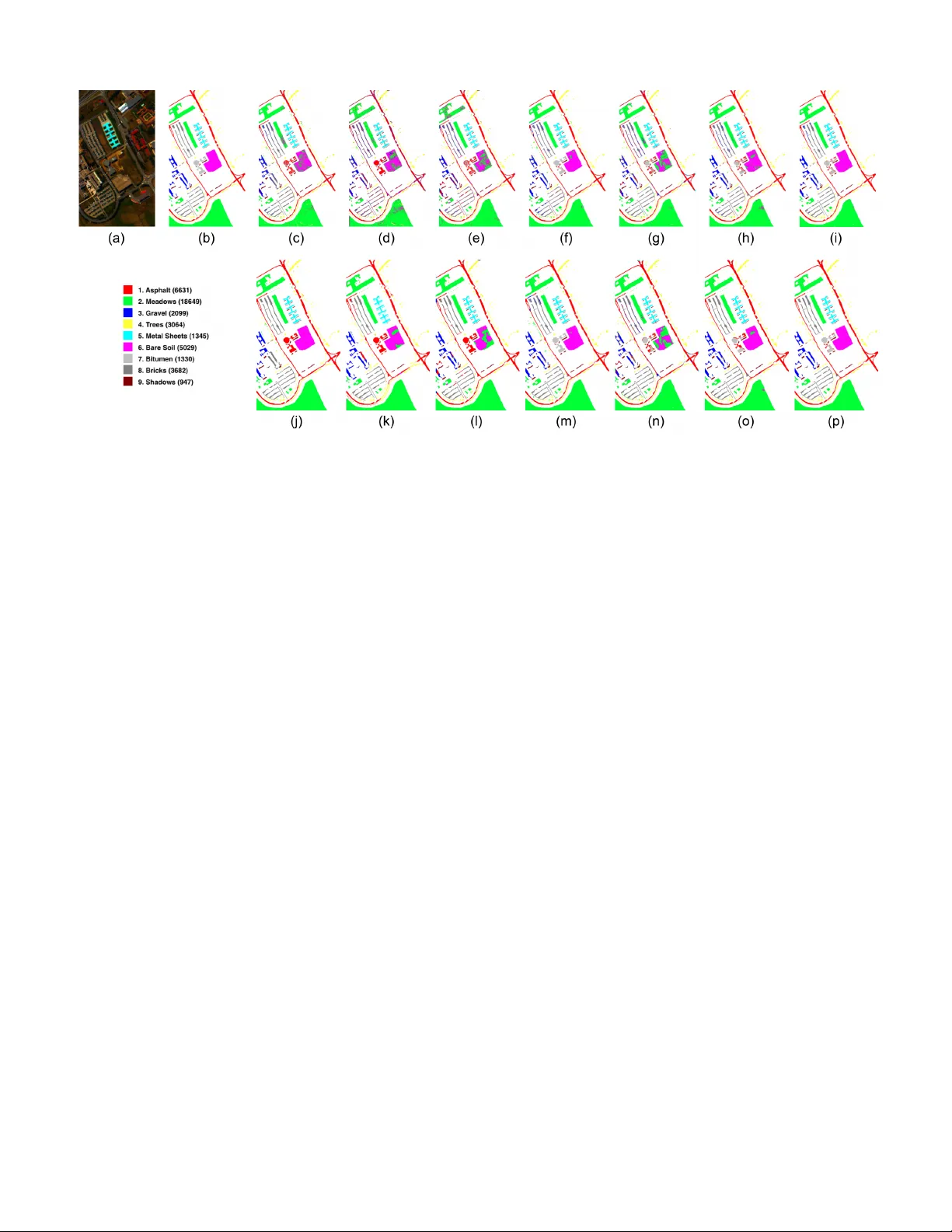
Generati v e Adv ersarial Networks and Conditional Random Fields for Hyperspectral Image Classification Zilong Zhong 1 , 2 , Jonathan Li 1 , 2 , 3 , David A. Clausi 1 , 2 , , Alexander W ong 1 , 2 1 Uni versity of W aterloo, W aterloo, ON, Canada 2 W aterloo Artificial Intelligence Institute, W aterloo, ON, Canada 3 Xiamen Uni versity , Xiamen, China Abstract In this paper , we address the hyperspectral image (HSI) classification task with a generativ e adversarial netw ork and conditional random field (GAN-CRF) -based frame work, which inte grates a semi-supervised deep learning and a probabilistic graphical model, and make three contrib utions. First, we design four types of con volutional and transposed conv olutional layers that consider the characteristics of HSIs to help with extracting discriminativ e features from limited numbers of labeled HSI samples. Second, we construct semi-supervised GANs to alle viate the shortage of training samples by adding labels to them and implicitly reconstructing real HSI data distribution through adversarial training. Third, we b uild dense conditional random fields (CRFs) on top of the random v ariables that are initialized to the softmax predictions of the trained GANs and are conditioned on HSIs to refine classification maps. This semi-supervised frame work leverages the merits of discriminativ e and generative models through a game-theoretical approach. Moreo ver , e ven though we used very small numbers of labeled training HSI samples from the two most challenging and extensiv ely studied datasets, the experimental results demonstrated that spectral-spatial GAN-CRF (SS-GAN-CRF) models achieved top-ranking accurac y for semi-supervised HSI classification. I . I N T RO D U C T I O N Due to their hundreds of spectral bands, the accurate interpretation of hyperspectral images (HSIs) has attracted significant scholarly attention from the machine learning and remote sensing communities [1]–[4]. Recent studies suggest that supervised deep learning models can alleviate challenges caused by the high spectral dimensionality of HSIs and achie ve strikingly better classification accuracy [5]–[7]. Howe ver , there are still three challenges that prev ent deep learning models from of fering precise pixel-wise HSI classification maps [8], [9]. First, the high dimensionality of HSI pixels make it hard to directly use the deep learning models for normal optical images in HSI interpretation. Second, the shortage of labeled pixels limits the classification performance of deep learning models. Third, the classification maps generated by deep learning models tend to be noisy and hav e spurious object edges. In this proposal, I will analyze these challenges and of fer our suggestions to mitigate them. The first challenge derives from the high spectral dimensionality of HSIs, which comprise two spatial dimensions and one spectral dimension. Conv entional methods focus on reducing the spectral dimensionality of HSIs. For example, [10] adopted dimensionality reduction methods to extract discriminativ e features for the con volutional neural networks (CNNs) that follow to classify . Nonetheless, these methods ignore the inherent dimension reduction capability of deep learning models. Many papers indicate that both spectral and spatial features play important roles in precise HSI interpretation. For instance, [9] employed a shared structured learning strate gy to construct a discriminant linear projection for spectral-spatial HSI classification. Additionally , [5] proposed an end-to-end CNN model for HSI classification and achie ved promising results, which show the generality of deep learning models. Howe ver , most machine learning models for HSI interpretation overlook the characteristics of this remotely sensed data. The second challenge stems from the high cost of and difficulty in obtaining a large amount of labeled data for HSIs. Deep learning models [11]–[13] are prevailing for HSI classification. Many papers suggest that these models require a large amount of training data. For e xample, [5] provided a method adding noise to HSI pixels in order to increase the number of training samples. Additionally , [11] proposed a pixel-pair approach that samples two pixels independently and couples them as a group for the purpose of enlarging the training data size. The scarcity of training samples is especially the case for some land cov er classes in HSI data sets. Howe ver , in contrast to the con ventional optical image classification objecti ves in the computer vision domain [14], [15], which usually contain hundreds or thousands of classes, the land cov er classification objecti ves of HSIs have far fewer classes to recognize. Therefore, the assumption that deep learning models require a high amount of data for training may not hold for HSIs. On the other hand, a large amount of unlabeled data remains an unexploited gold mine for efficient data use. Several works that focus on semi-supervised learning used small numbers of labeled and large numbers of unlabeled HSI samples for training. For instance, [16] adopted multi-layer neural networks to propagate labels from annotated HSI pixels Fig. 1: A semi-supervised GAN-CRF frame work for HSI classification. First, in the semi-supervised GAN, a generator transforms noise vectors z to a set of fake HSI cuboids Z , and a discriminator tries to distinguish the categorical information as well as the genuineness of input cuboids that come from X 1 or Z . Then, a dense CRF is established by using the softmax prediction of the trained discriminator about X 2 to initialize random v ariables Y , which is conditioned on the HSI data X . Mean field approximation is adopted to offer a refined classification map ˆ Y for the post-processing CRF . to unannotated ones. Moreover , [12] applied a stacked con volutional autoencoder to use spectral-spatial representation learned from other HSI datasets. Although this paper achieved accurate classification results, these results may originate from the large area of spatial information contained in each training sample rather than deep learning models. The third challenge is caused by the complexity of HSIs. Multiple works utilize the smoothness assumption that fa vors geometrically simple classification results [17]–[20]. For e xample, [18] incorporated a probabilistic graphical model as the post-processing step to improv e the classification outcomes of kernel support vector machines (SVMs). [21] constructed a conditional random field (CRF) with a high-order term to consider more complex relationships between different spectral bands and obtained very promising outcomes. Additionally , [19] incorporated a CRF for pre-processing as well as post- processing to stress the a priori smoothness and refine the classification maps. The adoption of probabilistic graphical models on top of supervised classification models can also be conceiv ed as a way to take the unlabeled samples into account for HSI classification because this step does not require the ground truth annotation of neighboring pixels. Howe ver , most CRF based models consider only the short-range correlations of pix els and ignore the long-range ones. In the face of these difficulties, two common semi-supervised learning methods — graph-based models and generati ve models — hav e been adopted to alleviate them [20], [22]–[24]. Graph-based models are premised on the smoothness assumption that accentuates geometrically simple classification results. F or example, [20] imposed a manifold re gularizer on a Laplacian SVM framew ork to learn spectral-spatial features for HSI image classification. Additionally , [22] proposed a dual hypergraph framew ork that imposes spectral-spatial constraints by jointly calculating a Laplacian matrix. Although these graph-based semi-supervised methods take both labeled and unlabeled samples into account, they identify HSI pixels based on hand-crafted features. Generally , these features learned from feature engineering steps are dif ficult to tune or generalize to other cases. Moreov er , the performance of these semi-supervised models lar gely depends on the quality of unlabeled data, which is hard to control or standardize. Recently , a generativ e model called generativ e adversarial network (GAN) [25] has attracted a lot of attention for image generation. For instance, [23] proposed a semi-supervised 1D-GAN for HSI classification, but ignored the spatial attribute of HSIs that can be used for enhancing classification performance. Moreov er , [24] used con volutional neural networks (CNNs) to build generativ e adversarial networks for HSI classification and achiev ed very promising results. Howe ver , the discriminators used in this paper only use three principled component analysis (PCA) channels of HSIs and therefore do not fully exploit the spectral characteristic of HSIs. Inspired by [25] and [26], we suggest a semi-supervised deep learning framework that consists of a generator , discriminator, and conditional random field built on top of the discriminator . The discriminator and generator form a generati ve adv ersarial network based on game theory . Specifically , the discriminator adopts spectral-spatial conv olutional layers to learn discriminative features from a small amount of labeled data and unlabeled data, and the generator employs spectral-spatial transposed con volutional layers to reconstruct HSI samples from vectors of Gaussian noise. Unlike traditional semi-supervised models, which require a large amount of unlabeled data for training, our proposed frame work is data-efficient because the generator creates a high amount of synthetic data and the discriminator takes a small number of unlabeled samples. In this way , the GAN-CRF model estimates the real data distribution, mitigates the shortage of annotated data, and smooths the semi-supervised Fig. 2: Four basic con volutional and transposed con volutional layers aiming for hyperspectral features extraction and generation in semi-supervised GAN-CRF models. (a) - (b) Spectral and spatial con v olutional layers in discriminators. (c) - (d) spectral and spatial transposed con volutional layers in generators. learning process. In addition, the output of the discriminator is the unary input term of the subsequent CRF . The binary term of the CRF imposes an a priori smoothness whereby adjacent pix els are more likely to belong to the same categories. More importantly , the CRF takes on a fully connected form that imposes a random field on the whole classification map and considers the long-range relationship between HSI pixels. Thus, by taking a generativ e adversarial network and considering the continuity of neighboring pixels, the designed semi-supervised architectures learn local fine-grain representation as well as high-lev el in variant features of HSI pixels concurrently . The main contributions of this study are as follows: 1) W e integrate the spectral-spatial attributes of HSIs into con volutional and transposed conv olutional layers of a GAN-CRF framew ork to learn discriminativ e spectral-spatial features of HSI samples. 2) W e construct semi-supervised GANs to alleviate the shortage of labeled data through adversarial training, which is a zero-sum game between the discriminators and generators of GANs. 3) W e b uild dense conditional random fields that impose graph constraints on the softmax predictions of trained discrimi- nators to refine HSI classification maps. The ov erall structure of this paper takes the form of fiv e sections: Section II revie ws related works with regard to the GAN- CRF framework. Section III introduces fundamental layers, spectral-spatial discriminators and generators, semi-supervised GANs, and post-processing CRFs of GAN-CRF models. Section IV offers model parameter settings, comparative experiments, and discussions. Last, section V makes some conclusions. I I . R E L A T E D W O R K GANs are unsupervised deep learning models that provide a solution to implicitly estimate real data distribution and correspondingly generate synthetic samples. Recently , there has been increasing interest in GANs for unsupervised learning, especially in regards to generating synthetic images that approximate the distribution of real ones [25], [27]. Compared with traditional generativ e methods, GANs are not constrained by Marko v fields or e xplicit approximation inference. F or instance, a deep con volutional GAN [28] that consists of deep conv olutional layers has been proposed to generate high-quality images. The original GAN aims for image generation and its variants have generated astonishing controllable and partially explainable images [29]. The GAN employs a discriminator and a generator to compete with each other . Specifically , the generator generates synthetic e xamples to deceive the discriminator , and the discriminator distinguishes real samples from fake ones. Since their objectiv es are contradictory , the training of the discriminator and generator of a GAN can be regarded as a process to find a Nash equilibrium through a game-theoretical point of view . Therefore, this GAN training can be formulated as a min-max optimization problem: min G max D Loss ( D , G ) = E x ∼ p data [log D ( x )] + E z ∼ p z [log (1 − D ( G ( z )))] , (1) where D ( · ) and G ( · ) represent softmax outputs of a discriminator and synthetic data generated by a generator, respectively . x and z denote true images and vectors of Gaussian noise, and they follow the distrib utions of real HSI data and Gaussian noise, respecti vely . GANs produce very promising image generation results in datasets like the MNIST digit database [30] and the Y ale F ace database [31], both of which contain compact data distribution and similar image layout. Graph models have widely been used for remotely sensed image interpretation tasks to effecti vely impose smoothness constraints on classification or segmentation results [26], [32]. CRFs are graphical models that assume a priori continuity whereby neighboring pixels of similar spectral signatures tend to have the same labels [21]. Since CRFs can be regarded as a structured generalization of multinomial logistic regression, the conditional probability distribution of a CRF takes this form: P rob ( y | x ) = exp( − E ( y | x )) P y exp( − E ( y | x )) , (2) Fig. 3: A spectral-spatial discriminator (upper), which comprises consecutiv e spectral and spatial feature learning blocks, outputs a v ector that contains a indicative entry of fake or real and categorical probabilities; and a spectral-spatial generator (lower), which comprises consecuti ve spectral and spatial feature generation blocks, transforms a vector of Gaussian noise to a synthetic HSI cuboid. where y and x denote output random variables and their corresponding observed data. E ( · ) is an energy function that models the joint probability distribution of y and x . The optimal random variables can be calculated by the maximum a posteriori (MAP) estimation: y M AP = arg max y P rob ( y | x ) . (3) Howe ver , although Equation (16) usually is an intractable problem, it can be solved through approximation methods [33]. I I I . P RO P O S E D M O D E L T o solve the three challenges of HSI classification, we propose a GAN-CRF -based semi-supervised deep learning framework. Suppose a hyperspectral image X contains m pixels { x i } ∈ R n x × m , where n x represents the number of spectral bands. Then, we sample two groups of HSI cuboids from X : the labeled group X 1 = { X 1 i } ∈ R n x × w × w × m l and the unlabeled group X 2 = { X 2 i } ∈ R n x × w × w × m u , where w , m l , and m u are the spatial width of HSI cuboids, the number of labeled, and the number of unlabeled HSI samples, respectively . Since each pixel in X corresponds to a HSI cuboid in { X 1 i , X 2 i } , therefore m = m l + m u . The labeled group X 1 has its annotation Y 1 = { y 1 i } ∈ R (1+ n y ) × m l , where n y is the number of land cov er classes and y 1 i [0] (the first entry in a vector y 1 i ) indicates whether the corresponding HSI cuboid is fake (1/0 means fake/real). As sho wn in Figure 1, the whole model is composed of a discriminator , a generator , and a post-processing CRF . Since annotations Y 1 of real HSI samples are used for training, the discriminator and generator form a semi-supervised GAN. The generator transforms noise vectors z to synthetic HSI cuboids Z = { Z i } , each sample of which hav e the same size as those from X 2 . The discriminator attempts to distinguish real HSI cuboids X 1 from fake ones Z and to classify real HSI cuboids. In contrast to updating one discriminativ e model in supervised deep learning, the training of a GAN in volves searching an equilibrium between the generator and discriminator by using stochastic gradient descent or similar methods to optimize the parameters of the GAN. Howe ver , GANs are known for their instability in training, and it is almost impossible to find an optimal equilibrium between their generators and discriminators. Therefore, we adopt an alternating optimization strategy that successiv ely updates the parameters of the generator and discriminator in each training iteration to help the discriminator to learn discriminative features using a small amount of labeled data and a large amount of synthetic data produced by the generator . When the training of a GAN is completed, we use the trained discriminator of the GAN to make a prediction about the unlabeled group X 2 . Then, a conditional random field is established by using the softmax predictions of the trained discriminator to initialize random variables Y = { y i } ∈ R (1+ n y ) × m that are conditioned on the raw HSI X . Last, we use mean field approximation to optimize the conditional random field and get a refined classification map ˆ Y . A. Spectral-Spatial Discriminator and Generator Discriminativ e deep learning models, such as CNNs and their extensions, hav e been used for HSI feature extraction and they hav e substantially outperformed traditional machine learning methods given enough training data [5], [6]. Howe ver , both these approaches ignore the inherent dif ference in spectral dimensionality between hyperspectral images and common images used in computer vision tasks. Based on the assumption that the sampled HSI data form a low dimensional manifold embedded in a higher dimensional space, multiple models ha ve tried to reduce the high dimensionality of HSI pix els and to learn more efficient representation [10], [34]. Howe ver , the dimension reduction process inevitably leads to the loss of useful information. The specialty of HSI samples lies in its high spectral dimensionality . Recently , in response to this characteristic, [6] implemented a spectral-spatial residual netw ork (SSRN) that considers the characteristics of HSI by consecutiv ely extracting spectral and spatial features and obtained state-of-the-art supervised classification results. Therefore, as illustrated in Figure 2 (a)-(b), we extend the idea of spectral and spatial conv olution from [6] to the discriminator of a GAN-CRF model. If X [ p +1] and X [ q +1] represent the feature tensors of [ p + 1] th spectral and [ q + 1] th spatial con volutional layers, then the spectral and spatial con volutional layers of a discriminator can be formulated as follo ws: X [ p +1] = LR eLU ( w [ p +1] ∗ X [ p ] + b [ p +1] ) , (4) X [ q +1] = LR eLU ( W [ q +1] ∗ X [ q ] + b [ q +1] ) , (5) where w [ p +1] and W [ q +1] represent the [ p + 1] th spectral and [ q + 1] th spatial con volutional kernels, respectively . b [ p +1] and b [ q +1] are the biases of these two layers. ∗ denotes the conv olutional operation. LReLU ( · ) is a leaky rectified linear unit function: LReLU ( a ) = ( a, if a > 0 , 0 . 2 a, otherwise . (6) In this work, we use padding tricks to keep the spatial size of feature tensors in most conv olutional layers unchanged. The goal of adopting spectral-spatial con volutional layers in a GAN-CRF model is to exploit as much information as possible from limited labeled HSI samples. Similarly , we stretch the spectral-spatial idea to transposed con volutional layers. As shown in Figure 2 (c)-(d), the spectral and spatial transposed conv olutional layers of a generator can be formulated as follo ws: z [ p +1] = R eLU ( h [ p +1] ∗ T z [ p ] + b [ p +1] ) , (7) Z [ q +1] = R eLU ( H [ q +1] ∗ T Z [ q ] + b [ q +1] ) , (8) where h [ p +1] and H [ q +1] represent the [ p + 1] th transposed spectral and [ q + 1] th transposed spatial con v olutional kernels. b [ p +1] and b [ q +1] are the biases of these two layers. ∗ T denotes the transposed conv olutional operation. ReLU ( · ) is the rectified linear unit function: ReLU ( a ) = ( a, if a > 0 , 0 , otherwise . (9) As shown in Figure 2, in contrast to spatial con volutional layers, the transposed conv olutional layers expand the spatial size of feature tensors. In both the discriminator and generator of a GAN-CRF model, we apply batch normalization [35] in all con volutional and transposed con volutional layers to stabilize the training of a GAN. B. Semi-supervised GAN A GAN can be regarded as a combination of discriminative and generative models, where the discriminator focuses on learning discriminativ e features, and the generator concentrates on implicitly reconstructing real data distribution from random noises. As an example of Uni versity of Pavia (UP) dataset shown in Figure 3, the discriminator comprises three spectral con volutional layers, three spatial conv olutional layers, and a fully connected layer before a v ector of softmax outputs. Con versely , the generator consists of a fully connected layer , three transposed spectral con volutional layers, and four spatial transposed con volutional layers to produce a synthetic hyperspectral cuboid. As the generator of a GAN can produce reasonable synthetic images and utilize them to train the discriminator of the GAN, many research papers hav e extended the discriminator of GANs to semi-supervised classification [23], [29], [36]. Similarly , we generalize the GAN to the semi-supervised HSI classification task. Since the labeled hyperspectral cuboid group X 1 = { X 1 i } has its corresponding annotation group Y 1 = { y 1 i } , the prediction of trained discriminators take this form: ˆ Y 1 = D ( X 1 ; θ D ) , (10) each element ˆ y 1 i of which has (1 + n y ) entries. Specifically , ˆ y 1 i [0] indicates the genuineness of a hyperspectral cuboid, and ˆ y 1 i [1 : n y ] is a vector of softmax outputs that shows the probabilities of a hyperspectral cuboid belonging to the n y land cover T ABLE I: Ov erall Accuracies (%) of semi-supervised GANs Using Dif ferent Numbers of Unlabeled and 200 Labeled HSI Samples in the IN and UP Datasets Datasets Models 0 1000 5000 IN SPC-GAN SP A-GAN SS-GAN 63 . 21 73 . 48 81 . 12 62 . 12 71 . 28 82 . 0 58 . 96 67 . 62 78 . 0 UP SPC-GAN SP A-GAN SS-GAN 84 . 24 91 . 01 96 . 96 84 . 69 91 . 74 95 . 76 79 . 17 87 . 35 93 . 90 classes. Compared to the original GAN that discriminates real data from fake ones, a semi-supervised GAN recognizes the categorical information of HSI cuboids by adding a supervised term to the loss function of a GAN. It is worth noting that the objecti ves of an unsupervised GAN and a semi-supervised GAN are different and ev en partially contradictory . The unsupervised GAN aims for implicitly estimating the true data distrib ution. On the contrary , the semi- supervised GAN focuses on data generation using limited labeled samples. Therefore, training a semi-supervised GAN jeopardize its image generation capability . As presented in [36], a good semi-supervised GAN requires a bad generator because this generator produces data outside real data distribution, which in turn helps the discriminator recognizes real data more accurately . In this w ay , the generator that produces synthetic HSI cuboids functions as a regularizer on the discriminator . Therefore, the loss function regarding optimize the discriminator of a GAN for semi-supervised HSI classification takes the form: L S E M I ( θ D , θ G ) = L S U P ( θ D ) + L D 1 ( θ D ) + L D 2 ( θ D , θ G ) , (11) where θ D and θ G are the parameters of a discriminator and a generator , respectiv ely . L S E M I is the total semi-supervised loss for training the discriminator of a semi-supervised GAN, L S U P , L D 1 , and L D 2 represent the supervised loss of a discriminator, the unsupervised loss of a discriminator , and the unsupervised loss of a generator , respectiv ely . These three terms are formulated as follows: L S U P ( θ D ) = − E X 1 ∼ p data log D ( X 1 ; θ D )[1 : n y ] = − E X 1 ∼ p data log ˆ Y 1 [1 : n y ] , (12) L D 1 ( θ D ) = − E X 1 ∼ p data log(1 − D ( X 1 ; θ D )[0]) = − E X 1 ∼ p data log(1 − ˆ Y 1 [0]) , (13) L D 2 ( θ D , θ G ) = − E z ∼ p z log D ( G ( z ; θ G ); θ D )[0] = − E z ∼ p z log D ( Z ; θ D )[0] = − E z ∼ p z log ˆ Y 1 [0] . (14) It is worth mentioning that L D 1 + L D 2 also is the part of the total semi-supervised loss L S E M I that aims at training the bad generator of a GAN [36]. Correspondingly , the loss function for training the generator of a semi-supervised GAN takes this form: L G ( θ D , θ G ) = − E z ∼ p z log (1 − D ( G ( z ; θ G ); θ D )[0]) = − E z ∼ p z log (1 − D ( Z ; θ D )[0]) = − E z ∼ p z log(1 − ˆ Y 1 [0]) . (15) The training of a semi-supervised GAN in volves two alternating steps of stochastic gradient descent (SGD) or similar optimization methods in each iteration. First, the gradients of a discriminator −∇ θ D L S E M I are used to update the parameters θ D of a discriminator for learning discriminati ve spectral-spatial HSI features. Second, the gradients of generators −∇ θ D L G are employed to update the parameters θ G of a generator for improving the adversarial training of the semi-supervised GAN. C. GAN-CRF Model CRFs ha ve been widely used to post-process image segmentation results because they can exploit the predictions of large numbers of unlabeled pix els to enhance image interpretation performance [17], [37]. Once a semi-supervised GAN has been Fig. 4: Overall accuracies of semi-supervised GANs with different kernel numbers in their con v olutiolnal and transposed con volutional layers using 300 labeled HSI samples for training. Fig. 5: Overall accuracies of semi-supervised GANs that contain varying depths of spectral and spatial con volutional layers in their discriminators using 300 labeled HSI samples for training . The x + y formation in the horizontal axis denotes a discriminator with x spectral and y spatial conv olutional layers. Fig. 6: Overall accuracies of different semi-supervised GANs and the supervised benchmark SS-CNNs using from 100 to 300 HSI samples for training. (a) IN dataset. (b) UP dataset. built, we establish a conditional random field by using the softmax predictions of the trained semi-supervised GAN about unlabeled HSI cuboids to initialize random variables Y = { y } that are conditioned on observed raw HSI pixels X . According T ABLE II: Classification Results, T raining, and T esting Times of Different Deep Learning Models Using 300 HSI Samples for the IN Dataset Class Samples 1D-GAN AE-GAN CNN-GAN SS-CNN SPC-GAN SP A-GAN SS-GAN 1 3 50 . 00 0 46 . 94 83 . 33 66 . 67 100 . 0 96 . 43 2 41 51 . 98 51 . 20 46 . 45 77 . 88 52 . 71 64 . 48 87 . 29 3 29 52 . 41 38 . 75 43 . 17 81 . 48 48 . 55 61 . 49 77 . 84 4 7 35 . 38 22 . 37 47 . 66 76 . 47 56 . 45 81 . 56 92 . 35 5 14 68 . 83 49 . 74 47 . 67 78 . 81 69 . 44 82 . 96 92 . 64 6 20 87 . 30 81 . 09 63 . 37 87 . 14 86 . 40 93 . 98 95 . 05 7 2 45 . 83 0 20 . 75 42 . 85 67 . 86 82 . 35 76 . 47 8 15 86 . 86 87 . 84 79 . 13 89 . 45 91 . 72 90 . 75 98 . 70 9 3 33 . 33 0 34 . 62 100 . 0 42 . 86 45 . 45 57 . 89 10 36 39 . 29 51 . 15 61 . 37 77 . 94 59 . 30 78 . 83 90 . 11 11 64 54 . 20 64 . 83 67 . 49 80 . 97 72 . 96 81 . 60 95 . 19 12 22 45 . 57 33 . 00 34 . 20 62 . 52 42 . 82 53 . 68 85 . 74 13 4 63 . 75 81 . 31 69 . 41 97 . 50 93 . 71 87 . 32 93 . 30 14 28 80 . 36 74 . 63 77 . 32 88 . 63 79 . 80 82 . 32 92 . 59 15 10 39 . 24 47 . 91 64 . 09 76 . 92 66 . 76 70 . 72 78 . 74 16 2 98 . 63 0 84 . 29 100 . 0 77 . 78 94 . 44 95 . 29 O A (%) 59 . 44 60 . 26 60 . 68 81 . 07 67 . 92 76 . 65 90 . 28 AA (%) 58 . 31 42 . 74 55 . 93 81 . 37 67 . 23 78 . 23 87 . 85 κ × 100 52 . 06 54 . 24 55 . 03 78 . 21 63 . 25 73 . 30 88 . 92 T raining (s) 153 . 85 217 . 70 64 . 87 139 . 55 932 . 23 233 . 32 803 . 23 T esting (s) 0 . 59 0 . 60 0 . 35 4 . 117 5 . 88 1 . 28 5 . 09 T ABLE III: Classification Results, T raining, and T esting Times of Different Deep Learning Models Using 300 HSI Samples for the UP Dataset Class Samples 1D-GAN AE-GAN CNN-GAN SS-CNN SPC-GAN SP A-GAN SS-GAN 1 47 84 . 74 62 . 51 73 . 38 96 . 07 84 . 74 91 . 10 95 . 62 2 132 92 . 50 92 . 02 90 . 17 97 . 57 87 . 31 96 . 93 99 . 49 3 15 75 . 75 39 . 25 58 . 09 72 . 82 60 . 77 78 . 84 89 . 02 4 20 93 . 46 84 . 55 98 . 39 99 . 37 97 . 07 98 . 94 98 . 65 5 11 99 . 55 94 . 72 99 . 41 98 . 97 95 . 06 99 . 55 100 . 0 6 35 86 . 77 62 . 72 74 . 21 98 . 18 86 . 70 92 . 71 99 . 09 7 13 82 . 43 40 . 46 89 . 29 96 . 38 85 . 86 95 . 76 97 . 10 8 21 73 . 79 51 . 78 83 . 65 82 . 81 75 . 85 86 . 88 92 . 54 9 6 98 . 13 66 . 14 99 . 30 99 . 36 96 . 56 99 . 79 100 . 0 O A (%) 88 . 36 75 . 10 84 . 23 95 . 04 85 . 78 93 . 97 97 . 61 AA (%) 87 . 46 66 . 02 85 . 10 93 . 50 85 . 55 93 . 39 96 . 84 κ × 100 84 . 41 67 . 07 78 . 79 93 . 40 80 . 69 91 . 98 96 . 82 T raining (s) 107 . 27 145 . 11 64 . 71 93 . 45 647 . 68 159 . 37 527 . 46 T esting (s) 2 . 06 1 . 34 1 . 76 14 . 30 18 . 38 4 . 03 15 . 36 to Equation (2), the conditional probability distribution of this CRF takes the form: P r ob ( y | X ) = exp( − E ( y | X )) P y exp( − E ( y | X )) . (16) As illustrated in Figure 1, giv en that high correlations exists between HSI pixels { x i } in both short- and long-range, we adopt a dense CRF [26] that includes all pairwise connections between HSI pix els in the pairwise term of energy function to filter salt and pepper noises in homogeneous areas. The ener gy function of the dense CRF can be formulated as: E ( Y | X ) = U ( Y , X ) + P ( Y , X ) , (17) where U ( · ) and P ( · ) are the unary and pairwise terms of the energy function that is used to build the dense CRF . Specifically , the unary term represents the information cost of pixel-wise softmax predictions { y i } and the binary term penalizes the wrong labeling of pixel pairs { x i , x j } with similar spectral signatures. These two terms are formulated as follows: U ( Y , X ) = X i U ( y i , X i ) = X i D ( X i ; θ D ) , (18) P ( Y , X ) = X i,j P ( y i , y j , x i , x j ) = X i,j µ ( y i , y j ) K ( x i , x j , l i , l j ) , (19) where l i and l j denote the locations of x i and x j , respectively . µ ( · ) is a compatibility function, and K ( · ) is a bilateral Gaussian kernel function. These two functions take the forms: µ ( y i , y j ) = ( c, if η ( y i ) 6 = η ( y j ) 0 , otherwise (20) K ( x i , x j , l i , l j ) = exp( − ( l i − l j ) 2 2 θ 2 α − ( x i − x j ) 2 2 θ 2 β ) , (21) where η ( · ) denotes a one-hot function. θ α and θ β are two standard deviations of the bilateral Gaussian function. c is a constant value that could be manually set. Random v ariables Y = { y i } of the established dense CRF is initialized to the softmax predictions of the trained discriminators D ( X 2 ; θ D ) of the semi-supervised GAN according to Equation (10). In a GAN-CRF model, a GAN is utilized to produce softax predictions about unlabeled HSI samples X 2 , and the post- processing CRF is independent of the GAN. Specifically , the predictions about a large numbers of unlabeled samples are used to initialize the unary term of the energy function that builds a dense CRF , and therefore the GAN-CRF model is more suitable in the case where only limited labeled samples are a v ailable. Because the ener gy function in Equation (17) is an intractable problem, a function Q ( Y | X ) adopted to approximate the conditional probability distrib ution P r ob ( Y | X ) of the CRF takes the form: Q ( Y | X ) = Y i Q ( y i | X ) ≈ P r ob ( Y | X ) , (22) in which the tractable function Q ( Y | X ) is close to P r ob ( Y | X ) in terms of KL-distribution diver gence. Then, the mean field approximation [33] is used to find an optimal solution of random variables ˆ Y for the established dense CRF . I V . R E S U LT A N D D I S C U S S I O N In this section, we introduce two challenging HSI datasets, set hyper-parameters of semi-supervised GANs, and ev aluate GAN-CRF models and their competitors using performance metrics including the classification accuracy of each land cov er class, ov erall accuracy (OA), a verage accuracy (AA), and kappa coef ficient ( κ ). Additionally , we record training and testing times of all semi-supervised GANs to quantitatively assess their computational complexity . A. Experimental Datasets T wo most challenging and commonly studied HSI datasets – the Indian Pines (IN) and the University of Pavia (UP) – are used to ev aluate the various types of semi-supervised GANs and GAN-CRF models for hyperspectral image classification. In both datasets, we randomly selected { 100 , 150 , 200 , 250 , 300 } HSI cuboids with their annotations for training, and used the remaining cuboids for testing. As shown in Figure 7 (a) - (b), the IN dataset contains 16 vegetation classes and has 145 × 145 pixels with a spatial resolution of 20 m by pixel. 200 hyperspectral bands are used for this study and they range from 400 nm to 2500 nm. As illustrated in Figure 8 (a) - (b), the UP dataset includes 9 urban land cover types and has 610 × 340 pix els with a spatial resolution of 1.3 m by pix el. 103 hyperspectral bands are used for this research and they range from 430 nm to 860 nm. The numbers of labeled HSI samples for each land cov er class for the IN and UP datasets can be found in Figure 7 and 8, respectiv ely . Giv en their relativ ely small numbers, the labeled hyperspectral groups X 1 used for training contain at least two samples for each land cov er class to av oid the situation that no sampled HSI cuboids are sampled for rare classes, especially in the IN dataset. B. Semi-supervised GAN Setting Figure 3 takes the UP dataset as an example to show the discriminator and generator of a semi-supervised GAN for HSI classification. In this semi-supervised GAN, the generator takes a 1 × 1 × 200 vector of Gaussian noise as the input and outputs a 9 × 9 × 103 fake HSI cuboid aiming to make the discriminator classify it as real data. Concurrently , a real 9 × 9 × 103 HSI cuboids is randomly sampled from a raw HSI as the input of the discriminator . In this study , according to the result of a grid search, we set the learning rate to 0 . 0007 , batch size to 50 , and the spatial size of sampled HSI cuboids to 9 × 9 . T o av oid model collapse, we used Monte Carlo sampling [29] to marginalize noise during training. Additionally , we adopted the Adam optimizer [38] to alternatingly train the discriminator and generator . After the hyper-parameters of semi-supervised GANs are configured, we analyzed three factors that influence the classification performance of semi-supervised GANs. First, the kernel number of con v olutional and transposed conv olutional layers affects the feature extraction and representation capacity of semi-supervised GANs. As illustrated in Figure 3, the discriminator and generator of a semi-supervised GAN have the same kernel number in its con volutional and transposed conv olutional layers. W e tested different kernel numbers from 16 to 32 in an interval of 4 for all con volutional or transposed con volutional layers of semi-supervised GANs. As shown in Figure 4, the semi-supervised GANs with 24 kernels in each layer achie ved the highest classification accuracy using the IN dataset, and their counterparts with 28 kernels obtained the best classification performance using the UP dataset. These results are acquired in the 3000-epoch training for both datasets using randomly sampled 300 HSI cuboids. Second, the depth of the spectral-spatial discriminators in semi-supervised GANs also impacts their classification perfor- mance. Therefore, we assessed semi-supervised GANs with from 4 to 8 layers, which includes spectral and spatial con volutional layers, with the same hyper-parameter setting for each dataset. T o make a fair comparison, we kept the generators of semi- supervised GANs hav e the same architecture as the generator in Figure 3. As demonstrated in Figure 5, the semi-supervised GANs with 3 spectral and 3 spatial con volutional layers obtained the highest ov erall accuracies in both datasets. The fact that classification performance of semi-supervised GANs decreases with more con volutional layers than the optimal ’ 3 + 3 ’ architecture shows discriminators with deeper layers overfit the small number of labeled real HSI samples. Third, to ev aluate the influence of unlabeled real HSI cuboids, we tested three types of semi-supervised GANs using different numbers of unlabeled HSI samples for the IN and UP datasets. The three semi-supervised GANs are the spectral GAN (SPC- GAN), and the spatial GAN (SP A-GAN), and the spectral-spatial GAN (SS-GAN). As sho wn in Figure 3, the SS-GAN has both spectral and spatial learning blocks in its discriminator , and the SPC-GAN and SP A-GAN contain only spectral and spatial blocks, respecti vely . Again, we used the same setting of generators for all semi-supervised GANs as the generator in Figure 3. T able I sho ws that adding real unlabeled HSI samples for training contrib utes little to and adding more unlabeled samples ev en jeopardizes the semi-supervised HSI classification accuracy , which is caused by the different data distrib ution between labeled and unlabeled HSI samples. C. Experimental Results W e compared the proposed semi-supervised GANs to state-of-the-art GAN-based models, such as 1D-GAN [23] , AE-GAN [12], and CNN-GAN [24]. T o demonstrate the effecti veness of the spectral-spatial architecture, we also compared spectral- spatial GANs (SS-GANs) that comprise three spectral and three spatial con volutional layers with their variants: SPC-GANs (three spectral layers) and SP A-GANs (three spatial layers). As shown in Figure 3, we recorded the HSI classification results of the spectral-spatial con volutional neural networks (SS-CNNs) as important benchmarks. W e kept the generators of all GANs the same, which consist of three spectral and four spatial transposed con volutions layers, each of which has 28 kernels. Then, we trained 3000 epochs for all GAN-based models, and set the input HSI cuboids with the same spatial size of 9 × 9 × for all methods that use spatial con volutional layers, and tuned the competitors to their optimal settings. T able II and T able III report the classification performance, including accuracy of all land cover classes, OAs, AAs, and Kappa coefficients, of the IN and UP datasets, respectiv ely . In most cases, the proposed semi-supervised GANs perform better than the state-of-the-art GAN-based models. Interestingly , the supervised benchmark SS-CNNs perform slightly better than SP A-GANs, which shows the discriminativ e feature learning capacity of spectral and spatial con volutional layers. More importantly , the SS-GANs achiev ed the highest overall classification accuracies ( 90 . 28% and 97 . 61% O As for the IN and UP datasets, respectively) among all GAN-based models and the SS-CNNs. It is worth noting that he semi-supervised SS-GANs outperform fully supervised SS-CNNs in IN and UP datasets with 9 . 21% and 2 . 57% , respectiv ely , which shows that the generated samples are helpful for improving classification accuracy . These results demonstrate the effecti veness of spectral- spatial con volutional architectures and semi-supervised adversarial training. Additionally , T able II and T able III also show the training and testing times of all models, which indicate the computational costs of these models. All experiments were conducted using an NVIDIA TIT AN Xp graphical processing unit (GPU). In both datasets, the SPC-GANs are the slowest to train and the SS-GANs take about 6 times longer for training than SS-CNNs. T o test the robustness of the SS-GANs and their competitors, we randomly sampled different numbers of labeled HSI cuboids in an interval of 50 from 100 to 300 to train these semi-supervised GANs and SS-CNNs for the IN and UP datasets. As shown in Figure 6, the classification performance of SP A-GANs is comparable to that of SS-CNNs. AE-GANs perform clearly worse than other models because their fully connected layers fail to take the spectral-spatial characteristics of HSI samples into account. More importantly , the proposed SS-GANs consistently outperform their semi-supervised competitors and SS-CNNs in both datasets. These results demonstrate the importance of accounting for the attributes of training data to design deep learning models, which is in line with the report of [6]. T ABLE IV: Overall Accuracies (%) of deep learning models and their refined results by adding dense CRFs using 300 labeled HSI samples for training IN Dataset UP Dataset Models w/o CRF w/ CRF w/o CRF w/ CRF 1D-GAN 59 . 44 70 . 41 88 . 36 94 . 41 AE-GAN 60 . 26 76 . 08 75 . 10 90 . 44 CNN-GAN 60 . 28 73 . 83 84 . 23 90 . 42 SS-CNN 81 . 07 87 . 66 95 . 04 98 . 05 SPC-GAN 68 . 92 74 . 64 85 . 78 88 . 13 SP A-GAN 76 . 65 85 . 64 93 . 97 97 . 57 SS-GAN 90 . 28 96 . 30 97 . 61 99 . 31 Fig. 7: Classification results of semi-supervised GAN models, a supervised CNN, and their refined counterparts by adding dense CRFs using 300 labeled HSI samples for the IN dataset. (a) False color image. (b) Ground truth labels. (c) - (i) Classification maps of 1D-GAN, AE-GAN, CNN-GAN, SS-CNN, SPC-GAN, SPC-GAN, and SS-GAN. (j) - (p) Classification maps of 1D-GAN-CRF , AE-GAN-CRF , CNN-GAN-CRF , SS-CNN-CRF , SPC-GAN-CRF , SP A-GAN-CRF , and SS-GAN-CRF . In this study , we used the three most prominent principal component analysis (PCA) channels of HSI X instead of raw HSI cuboids to facilitate the mean field approximation of the dense CRF . As sho wn in T able IV, SS-GANs and SS-GAN- CRF models perform better than their competitors, and GAN-CRF models significantly enhance the classification performance of those models without integrating dense CRFs, Moreov er , Figure 7 and Figure 8 sho w the classification maps of all semi- supervised GANs and all GAN-CRF models. The qualitativ e results of these classification maps are in line with the quantitativ e report of T able IV. The SS-GAN-CRF models deli ver the most accurate ov erall classification accuracies( 96 . 30% and 99 . 31% O As for the IN and UP datasets, respectiv ely) and smoothest classification maps for both HSI datasets, because the SS-GANs learn the most discriminati ve spectral-spatial features and dense CRFs consider long-range correlations between similar HSI samples. Therefore, these classification outcomes validate the feasibility of integrating semi-supervised deep learning and graph models giv en limited labeled HSI samples for training. D. Discussion There are three differences between the GAN-CRF framework and the original GAN proposed in [11]. First, GAN-CRF models take the spectral-spatial characteristics of HSI data into account for both the discriminators and generators. Second, the discriminators in the semi-supervised framework extend the softmax predictions ˆ y of a GAN from two classes (fake/real) to 1 + n y classes, where n y represents the number of land cov er classes. Third, a post-processing dense CRF has been b uilt on conditional random variables that are initialized to the softmax outputs of the trained GANs to filter salt and pepper noises in homogenous areas. The GAN-CRF models incorporate the CRF as a post-processing step and b uild a graph upon the learned features and the softmax outputs of discriminators to refine HSI classification maps. Compared with those CRFs adopted in pre vious articles [39], [40], the fully connected CRFs consider the long-range correlations between HSI samples. This property helps GAN-CRF models to better filter noises in the homogeneous areas of some land cover classes. Compared to just a supervised discriminator, a GAN-CRF model integrates the advantages of deep learning models and probabilistic graph models and improves HSI classification accuracy . There are two main reasons for this improvement: 1) the synthetic HSI samples produced by generators help discriminators to learn more robust and discriminative features; 2) the subsequent dense CRFs consider the spectral Fig. 8: Classification results of semi-supervised GAN models, a supervised CNN, and their refined counterparts by adding dense CRFs using 300 labeled HSI samples for the UP dataset. (a) False color image. (b) Ground truth labels. (c) - (i) Classification maps of 1D-GAN, AE-GAN, CNN-GAN, SS-CNN, SPC-GAN, SPC-GAN, and SS-GAN. (j) - (p) Classification maps of 1D-GAN-CRF , AE-GAN-CRF , CNN-GAN-CRF , SS-CNN-CRF , SPC-GAN-CRF , SP A-GAN-CRF , and SS-GAN-CRF . similarity and spatial closeness of HSI samples to refine the softmax outputs conditional on these samples using the trained discriminators of GANs. W e gain four major insights from the semi-supervised HSI classification outcomes of GANs and GAN-CRF models in both datasets. First, by taking the characteristics of training data into account, the discriminators of SS-GANs extract discriminative HSI features and achie ve better classification accurac y . Second, generators of SS-GANs learn feature representation by producing synthetic HSI samples, and in turn make discriminators more robust to adversaries and learn more discriminative features. Therefore, this adv ersarial training enables semi-supervised GANs to deli ver superior classification outcomes to supervised deep learning models. Third, adding unlabeled real HSI samples to train semi-supervised GANs marginally improves or even jeopardizes the HSI classification results. Fourth, dense CRFs take the classification maps generated by semi-supervised GANs as an initialization and smooth the noisy classification maps by adding a pairwise term that imposes the correlation between similar or neighboring pix els from input HSIs. V . C O N C L U S I O N In this paper , we have proposed a semi-supervised GAN-CRF frame work to address three commonly occurring challenges for HSI classification: the high spectral dimensionality of training data, the small numbers of labeled samples, and the noisy classification maps generated by deep learning models. First, we designed four consecuti vely structured con volutional and transposed con volutional layers to take the spectral-spatial characteristics of HSIs into consideration. Second, we established semi-supervised GANs, each of which comprises a generator and a discriminator , to extract discriminativ e features and to learn feature representation of HSI samples. Third, we integrated a probabilistic graphical model with a semi-supervised deep learning model to refine HSI classification maps. The e xperimental results using two of the most widely studied and challenging HSI datasets demonstrate that the spectral-spatial GANs (SS-GANs) perform the best among all semi-supervised GAN-based models and supervised benchmark models, and subsequently that the spectral-spatial GAN-CRF (SS-GAN-CRF) models achiev ed state-of-the-art performance for semi-supervised HSI classification. The GAN-CRF models demonstrate an effecti ve way to integrate two mainstream pixel-wise HSI classification methods — deep learning and probabilistic graphical models — and this framework can be easily generalized to other image interpretation cases. These two models have complementary advantages in the sense that deep learning models focus on discriminative feature extraction and implicit feature representation, and graph models emphasize the smoothness prior of images that is crucial for accurate classification and segmentation. Howe ver , the GAN-CRF framew ork presents a two-step setting because the dense CRFs function as a post-processing step to refine the classification maps generated by GANs. The contributions of this work mainly focus on validating the feasibility to integrate these two parts and show a way to implement this tar get. Therefore, a joint training framew ork is our future task, and current models need to be redesigned to achiev e this goal. For example, we could make the discriminator of GAN a local semantic segmentation network and change the generator accordingly . The reason of the separated training lies in the different roles of Semi-supervised GAN and fully-connected CRF . The GAN aims for training a discriminati ve model in a semi-supervised way and then using the trained model to generate pixelwise conditional probabilities. In contrast, the adoption of CRF considers the pixelwise classification prediction holistically and adds structural constraints on top of it. Therefore, we will continue this research line for imposing graph constraints on the con volutional layers of deep learning models to construct an end-to-end trainable framework. R E F E R E N C E S [1] H. Li, G. Xiao, T . Xia, Y . Y . T ang, and L. Li, “Hyperspectral image classification using functional data analysis, ” IEEE T rans. Cybern. , vol. 44, no. 9, pp. 1544–1555, 2014. [2] S. Jia, L. Shen, J. Zhu, and Q. Li, “ A 3-d gabor phase-based coding and matching framew ork for hyperspectral imagery classification, ” IEEE T rans. Cybern. , vol. 48, no. 4, pp. 1176–1188, 2018. [3] Y . Y uan, J. Lin, and Q. W ang, “Hyperspectral image classification via multitask joint sparse representation and stepwise mrf optimization, ” IEEE T rans. Cybern. , vol. 46, no. 12, pp. 2966–2977, 2016. [4] Y . Zhou and Y . W ei, “Learning hierarchical spectral–spatial features for hyperspectral image classification, ” IEEE T rans. Cybern. , vol. 46, no. 7, pp. 1667–1678, 2016. [5] Y . Chen, H. Jiang, C. Li, X. Jia, and P . Ghamisi, “Deep feature extraction and classification of hyperspectral images based on con volutional neural networks, ” IEEE T rans. Geosci. Remote Sens. , vol. 54, no. 10, pp. 6232–6251, 2016. [6] Z. Zhong, J. Li, Z. Luo, and M. Chapman, “Spectral-spatial residual network for hyperspectral image classification: A 3-d deep learning framew ork, ” IEEE Tr ans. Geosci. Remote Sens. , vol. 56, no. 2, pp. 847–858, 2018. [7] F . Luo, B. Du, L. Zhang, L. Zhang, and D. T ao, “Feature learning using spectral-spatial hypergraph discriminant analysis for hyperspectral image, ” IEEE T rans. Cybern. , vol. 49, no. 7, pp. 2406–2419, 2019. [8] Y . T arabalka, J. Chanussot, and J. A. Benediktsson, “Segmentation and classification of hyperspectral images using minimum spanning forest grown from automatically selected markers, ” IEEE T rans. Syst., Man, Cybern. B, Cybern. , vol. 40, no. 5, pp. 1267–1279, 2010. [9] H. Y uan and Y . Y . T ang, “Spectral–spatial shared linear regression for hyperspectral image classification, ” IEEE Tr ans. Cybern. , vol. 47, no. 4, pp. 934–945, 2017. [10] W . Zhao and S. Du, “Spectralspatial feature extraction for hyperspectral image classification: A dimension reduction and deep learning approach, ” IEEE T rans. Geosci. Remote Sens. , vol. 54, no. 8, pp. 4544–4554, 2016. [11] W . Li, G. Wu, F . Zhang, and Q. Du, “Hyperspectral image classification using deep pixel-pair features, ” IEEE T rans. Geosci. Remote Sens. , vol. 55, no. 2, pp. 844–853, 2017. [12] Y . Chen, Z. Lin, X. Zhao, G. W ang, and Y . Gu, “Deep learning-based classification of hyperspectral data, ” IEEE J. Sel. T opics Appl. Earth Observ . Remote Sens. , vol. 7, no. 6, pp. 2094–2107, 2014. [13] Y . Chen, X. Zhao, and X. Jia, “Spectral-spatial classification of hyperspectral data based on deep belief network, ” IEEE J. Sel. T opics Appl. Earth Observ . Remote Sens. , vol. 8, no. 6, pp. 2381–2392, 2015. [14] A. Krizhevsky , I. Sutskev er , and G. E. Hinton, “Imagenet classification with deep conv olutional neural networks, ” in in Pr oc. Adv . Neural Inf. Process. Syst. , Conference Proceedings, pp. 1106–1114. [15] Y . LeCun, Y . Bengio, and G. Hinton, “Deep learning, ” Nature , vol. 521, no. 7553, pp. 436–444, 2015. [16] V . Mnih, K. Kavukcuoglu, D. Silver, A. A. Rusu, J. V eness, M. G. Bellemare, A. Graves, M. Riedmiller, A. K. Fidjeland, and G. Ostrovski, “Human-level control through deep reinforcement learning, ” Nature , vol. 518, no. 7540, pp. 529–533, 2015. [17] X. Cao, F . Zhou, L. Xu, D. Meng, Z. Xu, and J. Paisley , “Hyperspectral image classification with markov random fields and a con volutional neural network, ” IEEE T rans. Image Process. , vol. 27, no. 5, pp. 2354–2367, 2018. [18] Y . T arabalka, M. Fauvel, J. Chanussot, and J. A. Benediktsson, “Svm- and mrf-based method for accurate classification of hyperspectral images, ” IEEE T rans. Geosci. Remote Sens. Lett. , vol. 7, no. 4, pp. 736–740, 2010. [19] Y . Zhong, J. Zhao, and L. Zhang, “ A hybrid object-oriented conditional random field classification framew ork for high spatial resolution remote sensing imagery , ” IEEE T rans. Geosci. Remote Sens. , vol. 52, no. 11, pp. 7023–7037, 2014. [20] L. Y ang, S. Y ang, P . Jin, and R. Zhang, “Semi-supervised hyperspectral image classification using spatio-spectral laplacian support vector machine, ” IEEE Tr ans. Geosci. Remote Sens. Lett. , vol. 11, no. 3, pp. 651–655, 2014. [21] P . Zhong and R. W ang, “Modeling and classifying hyperspectral imagery by crfs with sparse higher order potentials, ” IEEE Tr ans. Geosci. Remote Sens. , vol. 49, no. 2, pp. 688–705, 2011. [22] R. Ji, Y . Gao, R. Hong, Q. Liu, D. T ao, and X. Li, “Spectral-spatial constraint hyperspectral image classification, ” IEEE Tr ansactions on Geoscience and Remote Sensing , vol. 52, no. 3, pp. 1811–1824, 2014. [23] Y . Zhan, D. Hu, Y . W ang, and X. Y u, “Semisupervised hyperspectral image classification based on generative adversarial networks, ” IEEE T rans. Geosci. Remote Sens. Lett. , vol. 15, no. 2, pp. 212–216, 2018. [24] L. Zhu, Y . Chen, P . Ghamisi, and J. A. Benediktsson, “Generative adversarial networks for hyperspectral image classification, ” IEEE Tr ans. Geosci. Remote Sens. , 2018. [25] I. Goodfellow , J. Pouget-Abadie, M. Mirza, B. Xu, D. W arde-Farley , S. Ozair, A. Courville, and Y . Bengio, “Generative adversarial nets, ” in in Proc. Adv . Neural Inf. Process. Syst. , 2014, pp. 2672–2680. [26] L.-C. Chen, G. Papandreou, I. Kokkinos, K. Murphy , and A. L. Y uille, “Deeplab: Semantic image segmentation with deep con volutional nets, atrous con volution, and fully connected crfs, ” IEEE T rans. P attern Anal. Mach. Intell. , vol. 40, no. 4, pp. 834–848, 2018. [27] T . Salimans, I. Goodfellow , W . Zaremba, V . Cheung, A. Radford, and X. Chen, “Improved techniques for training gans, ” in in Proc. Adv . Neural Inf. Pr ocess. Syst. , 2016, pp. 2234–2242. [28] A. Radford, L. Metz, and S. Chintala, “Unsupervised representation learning with deep conv olutional generative adversarial networks, ” arXiv preprint arXiv:1511.06434 , 2015. [29] Y . Saatci and A. G. Wilson, “Bayesian gan, ” in in Proc. Adv . Neural Inf. Pr ocess. Syst. , 2017, pp. 3622–3631. [30] Y . LeCun, L. Bottou, Y . Bengio, and P . Haffner , “Gradient-based learning applied to document recognition, ” Pr oc. IEEE , vol. 86, no. 11, pp. 2278–2324, 1998. [31] J. Y ang, D. Zhang, A. F . Frangi, and J.-y . Y ang, “T wo-dimensional pca: a new approach to appearance-based face representation and recognition, ” T rans. P attern Anal. Mach. Intell. , vol. 26, no. 1, pp. 131–137, 2004. [32] J. Zhao, Y . Zhong, H. Shu, and L. Zhang, “High-resolution image classification integrating spectral-spatial-location cues by conditional random fields, ” IEEE Tr ans. Image Pr ocess. , vol. 25, no. 9, pp. 4033–4045, 2016. [33] P . Kr ¨ ahenb ¨ uhl and V . K oltun, “Efficient inference in fully connected crfs with gaussian edge potentials, ” in in Pr oc. Adv . Neural Inf. Process. Syst. , 2011, pp. 109–117. [34] L. Zhang, L. Zhang, D. T ao, X. Huang, and B. Du, “Hyperspectral remote sensing image subpixel target detection based on supervised metric learning, ” IEEE Tr ans. Geosci. Remote Sens. , vol. 52, no. 8, pp. 4955–4965, 2014. [35] S. Ioffe and C. Szegedy , “Batch normalization: Accelerating deep network training by reducing internal covariate shift, ” in in Pr oc. 32nd Int. Conf. on Mach. Learn. , pp. 448–456. [36] Z. Dai, Z. Y ang, F . Y ang, W . W . Cohen, and R. R. Salakhutdinov , “Good semi-supervised learning that requires a bad gan, ” in in Proc. Adv . Neural Inf. Pr ocess. Syst. , 2017, pp. 6513–6523. [37] S. Zheng, S. Jayasumana, B. Romera-Paredes, V . V ineet, Z. Su, D. Du, C. Huang, and P . H. T orr , “Conditional random fields as recurrent neural networks, ” in Proc. IEEE Conf. Comput. V is. P attern Recognit. , 2015, pp. 1529–1537. [38] D. P . Kingma and J. Ba, “ Adam: A method for stochastic optimization, ” arXiv preprint , 2014. [39] P . Zhong and R. W ang, “Learning conditional random fields for classification of hyperspectral images, ” IEEE T rans. Image Process. , vol. 19, no. 7, pp. 1890–1907, 2010. [40] J. Zhao, Y . Zhong, and L. Zhang, “Detail-preserving smoothing classifier based on conditional random fields for high spatial resolution remote sensing imagery , ” IEEE T rans. Geosci. Remote Sens. , vol. 53, no. 5, pp. 2440–2452, 2015.