Smooth minimization of nonsmooth functions with parallel coordinate descent methods

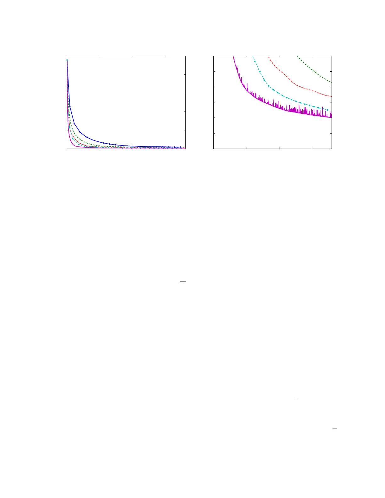
Smo oth Minimization of Nonsmo oth F unctions with P arallel Co ordinate Descen t Metho ds Olivier F erco q ∗ P eter Rich t´ arik † Septem b er 22, 2013 Abstract W e study the p erformance of a family of randomized parallel co ordinate descent methods for minimizing the sum of a nonsmo oth and separable con vex functions. The problem class includes as a sp ecial case L1-regularized L1 regression and the minimization of the exponential loss (“AdaBoost problem”). W e assume the input data defining the loss function is contained in a sparse m × n matrix A with at most ω nonzeros in each ro w. Our metho ds need O ( nβ /τ ) iterations to find an appro ximate solution with high probability , where τ is the n umber of pro cessors and β = 1 + ( ω − 1)( τ − 1) / ( n − 1) for the fastest v arian t. The notation hides dep endence on quantities such as the required accuracy and confidence levels and the distance of the starting iterate from an optimal point. Since β /τ is a decreasing function of τ , the method needs few er iterations when more pro cessors are used. Certain v ariants of our algorithms p erform on av erage only O (nnz( A ) /n ) arithmetic op erations during a single iteration p er pro cessor and, b ecause β decreases when ω do es, fewer iterations are needed for sparser problems. 1 In tro duction It is increasingly common that practitioners in mac hine learning, optimization, biology , engineering and v arious industries need to solv e optimization problems with n umber of v ariables/coordinates so h uge that classical algorithms, which for historical reasons almost in v ariably fo cus on obtaining solutions of high accuracy , are not efficien t enough, or are outright unable to p erform even a single iteration. Indeed, in the big data optimization setting, where the n umber N of v ariables is huge, in version of matrices is not p ossible, and even op erations suc h as matrix v ector m ultiplications are to o exp ensiv e. Instead, attention is shifting to wards simple metho ds, with c heap iterations, low memory requiremen ts and go od parallelization and scalabilit y prop erties. If the accuracy requirements are mo derate and the problem has only simple constraints (suc h as b ox constraints), metho ds with these prop erties do exist: p ar al lel c o or dinate desc ent metho ds [2, 23, 26, 33] emerged as a v ery promising class of algorithms in this domain. ∗ Sc ho ol of Mathematics, The Universit y of Edin burgh, United Kingdom (e-mail: olivier.ferco q@ed.ac.uk) † Sc ho ol of Mathematics, The Univ ersity of Edinburgh, United Kingdom (e-mail: p eter.ric h tarik@ed.ac.uk) The work of b oth authors was supported b y the EPSR C grant EP/I017127/1 (Mathematics for V ast Digital Re- sources). The work of P .R. was also supp orted by the Centre for Numerical Algorithms and Intelligen t Soft ware (funded by EPSR C gran t EP/G036136/1 and the Scottish F unding Council). 1 1.1 P arallel co ordinate descent metho ds In a recent pap er [26], Ric ht´ arik and T ak´ a ˇ c prop osed and studied the complexit y of a p ar al lel c o or dinate desc ent metho d (PCDM) applied to the con vex comp osite 1 optimization problem min x ∈ R N φ ( x ) + Ψ( x ) , (1) where φ : R N → R is an arbitr ary differ entiable con vex function and Ψ : R N → R ∪ { + ∞} is a simple (blo c k) sep ar able conv ex regularizer, such as λ k x k 1 . The N v ariables/coordinates of x are assumed to b e partitioned into n blo c ks, x (1) , x (2) , . . . , x ( n ) and PCDM at eac h iteration computes and applies up dates to a randomly chosen subset ˆ S ⊆ [ n ] def = { 1 , 2 , . . . , n } of blo c ks (a “sampling”) of the decision vector, in p ar al lel . F ormally , ˆ S is a random set-v alued mapping with v alues in 2 [ n ] . PCDM enco des a family of algorithms where each v arian t is characterized b y the probability la w gov erning ˆ S . The sets generated throughout the iterations are assumed to b e indep enden t and iden tically distributed. In this pap er we fo cus on uniform samplings , which are characterized by the requiremen t that P ( i ∈ ˆ S ) = P ( j ∈ ˆ S ) for all i, j ∈ [ n ]. It is easy to see that for a uniform sampling one necessarily has 2 P ( i ∈ ˆ S ) = E [ | ˆ S | ] n . (2) In particular, we will fo cus on t wo sp ecial classes of uniform samplings: i) those for whic h P ( | ˆ S | = τ ) = 1 ( τ -uniform samplings ), and ii) τ -uniform saplings with the additional prop ert y that all subsets of cardinalit y τ are chosen equally likely ( τ -nic e samplings ). W e will also say that a sampling is pr op er if P ( | ˆ S | ≥ 1) > 0. It is clearly imp ortan t to understand whether choosing τ > 1, as opposed to τ = 1, leads to acceleration in terms of an improv ed complexit y b ound. Ric ht´ arik and T ak´ aˇ c [26, Section 6] established generic iter ation c omplexity r esults for PCDM applied to (1)—we describ e them in some detail in Section 1.3. Let us only mention no w that these results are generic in the sense that they hold under the blanket assumption that a certain inequality in volving φ and ˆ S holds, so that if one is able to derive this inequalit y for a certain class of smo oth conv ex functions φ , complexity results are readily av ailable. The inequality (called Exp ected Separable Ov erapproximation, or ESO) is E h φ ( x + h [ ˆ S ] ) i ≤ φ ( x ) + E [ | ˆ S | ] n h∇ φ ( x ) , h i + β 2 n X i =1 w i h B i h ( i ) , h ( i ) i ! , x, h ∈ R N , (3) where B i are p ositiv e definite matrices (these can b e chosen based on the structure of φ , or simply tak en to b e iden tities), β > 0, w = ( w 1 , . . . , w n ) is a v ector of p ositiv e weigh ts, and h [ ˆ S ] denotes the random v ector in R N obtained from h b y zeroing out all its blo c ks that do not b elong to ˆ S . That is, h [ S ] is the vector in R N for which h ( i ) [ S ] = h ( i ) if i ∈ S and h ( i ) [ S ] = 0, otherwise. When (3) holds, we sa y that φ admits a ( β , w )-ESO with resp ect to ˆ S . F or simplicity , w e may sometimes write ( φ, ˆ S ) ∼ ESO( β , w ). Let us now give the intuition b ehind the ESO inequalit y (3). Assuming the current iterate is x , PCDM c hanges x ( i ) to x ( i ) + h ( i ) ( x ) for i ∈ ˆ S , where h ( x ) is the minimizer of the right hand side of (3). By doing so, we b enefit from the following: 1 Gradien t methods for problems of this form w ere studied by Nestero v [21]. 2 This and other identities for blo c k samplings were derived in [26, Section 3]. 2 (i) Since the o verappro ximation is a conv ex quadratic in h , it e asy to c ompute h ( x ). (ii) Since the o v erapproximation is blo c k separable, one c an c ompute the up dates h ( i ) ( x ) in p ar al lel for all i ∈ { 1 , 2 , . . . , n } . (iii) F or the same reason, one c an c ompute the up dates or i ∈ S k only , where S k is the sample set dra wn at iteration k following the law describing ˆ S . The algorithmic strategy of PCDM is to mo ve to a new p oin t in such a w a y that the exp ected v alue of the loss function ev aluated at this new p oin t is as small as p ossible. The metho d effectiv ely decomp oses the N -dimensional problem into n smaller conv ex quadratic problems, attending to a random subset of τ of them at each iteration, in parallel. A single iteration of PCDM can b e compactly written as x ← x + ( h ( x )) [ ˆ S ] , (4) where h ( x ) = ( h (1) ( x ) , . . . , h ( n ) ( x )) and h ( i ) ( x ) = arg min h  h ( ∇ φ ( x )) ( i ) , h ( i ) i + β w i 2 h B i h ( i ) , h ( i ) i  (3) = − 1 β w i B − 1 i ( ∇ φ ( x )) ( i ) . (5) F rom the up date formula (5) w e can see that 1 β can b e interpreted as a stepsize. W e would hence wish to c ho ose small β , but not to o small so that the metho d do es not div erge. The issue of the computation of a go od (small) parameter β is v ery intricate for several reasons, and is at the heart of the design of a randomized parallel co ordinate descent metho d. Muc h of the theory dev elop ed in this pap er is aimed at iden tifying a class of nonsmo oth comp osite problems which, when smo othed, admit ESO with a small and easily computable v alue of β . In the following text w e give some insigh t into why this issue is difficult, still in the simplified smo oth setting. 1.2 Spurious w a ys of computing β Recall that the parameters β and w giving rise to an ESO need to be explicitly c alculate d b efore the metho d is run as they are needed in the computation of the up date steps. W e will now describe the issues associated with finding suitable β , for simplicity assuming that w has been c hosen/computed. 1. Let us start with a first approach to computing β . If the gradient of φ is Lipsc hitz with resp ect to the separable norm k x k 2 w def = n X i =1 w i h B i x ( i ) , x ( i ) i , with known Lipschitz constant L , then for all x, h ∈ R N w e hav e φ ( x + h 0 ) ≤ φ ( x ) + h∇ φ ( x ) , h 0 i + L 2 k h 0 k 2 w . Now, if for fixed h ∈ R N w e substitute h 0 = h [ ˆ S ] in to this inequalit y , and tak e exp ectations utilizing the identities [26] E h h x, h [ ˆ S ] i i = E [ | ˆ S | ] n h x, h i , E h k h [ ˆ S ] k 2 w i = E [ | ˆ S | ] n k h k 2 w , (6) w e obtain ( φ, ˆ S ) ∼ ESO( β , w ) for β = L . It turns out that this w ay of obtaining β is far from satisfactory , for several reasons. 3 (a) First, it is very difficult to compute L in the big data setting PCDMs are designed for. In the case of L2 regression, for instance, L will b e equal to the largest eigenv alue of a certain N × N matrix. F or huge N , this is a formidable task, and may actually b e harder than the problem we are trying to solve. (b) W e sho w in Section 4.1 that taking β = n τ c , where c is a b ound on the Lipsc hitz constan ts (with resp ect to the norm k · k w , at h = 0, uniform in x ) of the gradients of the functions h → E [ φ ( x + h [ ˆ S ] )] precisely characterizes (3), and leads to smaller (=b etter) v alues β . Surprisingly , this β can b e O ( √ n ) times smaller than L . As w e shall see, this directly translates in to iteration complexit y sp eedup by the factor of O ( √ n ). 2. It is often easy to obtain go o d β in the case τ = 1. Indeed, it follows from [19, 24] that any smo oth conv ex function φ will satisfy (3) with β = 1 and w i = L i , where L i is the blo c k Lipsc hitz constan t of the gradient of φ with resp ect to the norm h B i · , ·i 1 / 2 , asso ciated with blo c k i . If the size of blo c k i is N i , then the computation of L i will typically amount to the finding a maximal eigenv alue of an N i × N i matrix. If the blo c k sizes N i are sufficiently small, it is muc h simpler to compute n of these quan tities than to compute L . No w, can w e use a similar technique to obtain β in the τ > 1 case? A naive idea would b e to k eep β unc hanged ( β = 1). In view of (5), this means that one w ould simply compute the up dates h ( i ) ( x ) in the same wa y as in the τ = 1 case, and apply them all. How ev er, this strategy is do omed to fail: the metho d ma y end up oscillating b et ween sub-optimal p oin ts (a simple 2 dimensional example w as describ ed in [33]). This issue arises since the algorithm o vershoots: while the individual up dates are safe for τ = 1, it is not clear why adding them all up for arbitrary τ should decrease the function v alue. 3. A natural remedy to the problem describ ed in § 2 is to decrease the stepsize, i.e., to increase β as τ increases. In fact, it can b e inferred from [26] that β ( τ ) = τ alwa ys works: it satisfies the ESO inequality and the metho d conv erges. This makes intuitiv e sense since the actual step in the τ > 1 case is obtained as the aver age of the blo c k updates which are safe in the τ = 1 case. By Jensen’s inequality , this must decrease the ob jectiv e function since the randomized serial metho d do es (b elo w we assume for notational simplicity that all blo c ks are of size one, e i are the unit co ordinate v ectors): φ ( x + ) = φ   x − X i ∈ ˆ S 1 τ L i ( ∇ φ ( x )) ( i ) e i   ≤ 1 τ X i ∈ ˆ S φ  x − 1 L i ( ∇ φ ( x )) ( i ) e i  . Ho wev er, this approac h comp ensates the increase of computational p o wer ( τ ) b y the same decrease in stepsize, which means that the parallel metho d ( τ > 1) migh t in the worst case require the same num b er of iterations as the serial one ( τ = 1). 4. The issues describ ed in § 2 and § 3 lead us to the follo wing question: Is it p ossible to safely and quickly choose/compute a v alue of β in the τ = 1 case which is larger than 1 but smaller than τ ? If this was p ossible, we could exp ect the parallel metho d to b e muc h b etter than its serial counterpart. An affirmative answer to this question for the class of smo oth conv ex partially separable functions φ was given in [26]. 4 T o summarize, the issue of selecting β in the parallel setting is very in tricate, and of utmost significance for the algorithm. In the next t wo subsections w e now giv e more insight into this issue and in doing so progress into discussing our contributions. 1.3 Generic complexit y results and partial separability The generic complexity results mentioned earlier, established in [26] for PCDM, hav e the form 3 k ≥  β τ  × n × c ⇒ P  φ ( x k ) − min x φ ( x ) ≤   ≥ 1 − ρ, where c is a constan t indep enden t of τ , and dep ending on the error tolerance  , confidence tolerance ρ , initial iterate x 0 , optimal p oin t x ∗ and w . Moreov er, c do es not hide any large c onstan ts. Keeping τ fixed, from (5) we see that larger v alues of β lead to smaller stepsizes. W e commen ted earlier, app ealing to intuition, that this translates into worse complexity . This is now affirmed and quan tified by the ab o ve generic complexity result. Note, how ever, that this generic result do es not pr ovide any c oncr ete information ab out p ar al lelization sp e e dup b ecause it do es not say anything ab out the dep endence of β on τ . Clearly , parallelization sp eedup o ccurs when the function T ( τ ) = β ( τ ) τ is decreasing. The b eha vior of this function is imp ortan t for big data problems whic h can only b e solv ed by decomp osition metho ds, suc h as PCDM, on mo dern HPC arc hitectures. Besides proving generic complexit y b ounds for PCDM, as outlined ab o v e, Rich t´ arik and T ak´ a ˇ c [26] identified a class of smo oth c onvex functions φ for which β can b e explicitly computed as a function of τ in closed form, and for which indeed T ( τ ) is decreasing: p artial ly sep ar able functions. A conv ex function φ : R N → R is partially separable of degree ω if it can b e written as a sum of differen tiable 4 con vex functions, each of whic h depends on at most ω of the n blo cks of x . If ˆ S is a τ - uniform sampling, then β = β 0 = min { ω , τ } . If ˆ S is a τ -nice sampling, then β = β 00 = 1 + ( ω − 1)( τ − 1) n − 1 . Note that β 00 ≤ β 0 and that β 0 can b e arbitrarily larger than β 00 . Indeed, the w orst case situation (in terms of the ratio β 0 β 00 ) for any fixed n is ω = τ = √ n , in which case β 0 β 00 = 1 + √ n 2 . This means that PCDM implemen ted with a τ -nice sampling (using β 00 ) can b e arbitrarily faster than PCDM implemented with the more general τ -uniform sampling (using β 0 ). This simple example illustrates the huge impact the choice of the sampling ˆ S has, other things equal. As we shall sho w in this paper, this phenomenon is directly related to the issue w e discussed in Section 1.2: L can b e O ( √ n ) times larger than a go o d β . 3 This holds provided w do es not change with τ ; which is the case in this pap er and in the smo oth partially separable setting considered in [26, Section 6]. Also, for simplicity w e cast the results here in the case Ψ ≡ 0, but they hold in the comp osite case as w ell. 4 It is not assumed that the summands hav e Lipschitz gradient. 5 1.4 Brief literature review Serial randomized metho ds. Leven thal and Lewis [10] studied the complexit y of randomized co ordinate descen t metho ds for the minimization of conv ex quadratics and prov ed that the metho d con verges linearly ev en in the non-strongly con vex case. Linear conv ergence for smo oth strongly con vex functions w as pro ved b y Nestero v [19] and for general regularized problems b y Ric h t´ arik and T ak´ aˇ c [24]. Complexity results for smo oth problems with sp ecial regularizes (b ox constraints, L1 norm) w ere obtained b y Shalev-Shw arz and T ewari [30] and Nesterov [19]. Nesterov was the first to analyze the blo c k setting, and prop osed using different Lipsc hitz constants for differen t blo c ks, whic h has a big impact on the efficiency of the metho d since these constants capture imp ortant second order information [19]. Also, he w as the first to analyze an accelerated co ordinate descent metho d. Rich t´ arik and T ak´ aˇ c [25, 24] improv ed, generalized and simplified previous results and extended the analysis to the composite case. They also gav e the first analysis of a co ordinate descent metho d using arbitrary probabilities. Lu and Xiao [11] recently studied the w ork dev elop ed in [19] and [26] and obtained further impro vemen ts. Co ordinate descent metho ds were recen tly extended to deal with coupled constraints b y Necoara et al [16] and extended to the comp osite setting b y Necoara and P atrascu [17]. When the function is not smooth neither comp osite, it is still p ossible to define co ordinate descent metho ds with subgradients. An algorithm based on the av eraging of past subgradien t co ordinates is presen ted in [34] and a successful subgradien t-based co ordinate descen t metho d for problems with sparse subgradien ts is prop osed by Nestero v [20]. T app enden et al [36] analyzed an inexact randomized coordinate descent method in whic h proximal subproblems at eac h iteration are solved only approximately . Dang and Lan [4] studied complexity of sto c hastic blo ck mirror descent metho ds for nonsmo oth and stochastic optimization and an accelerated method w as studies by Shalev-Shw arz and Zhang [31]. Lacoste-Julien et al [9] were the first to dev elop a blo c k-co ordinate F rank-W olfe metho d. The generalized p o w er metho d of Journ´ ee et al [8] designed for sparse PCA can b e seen as a nonconv ex blo c k co ordinate ascent metho d with tw o blo cks [27]. P arallel metho ds. One of the first complexit y results for a parallel coordinate descen t metho d w as obtained b y Ruszczy ´ nski [28] and is known as the diagonal quadratic appro ximation metho d (DQAM). DQAM up dates all blo c ks at eac h iteration, and hence is not randomized. The metho d w as designed for solving a con vex comp osite problem with quadratic smo oth part and arbitrary sep- arable nonsmo oth part and w as motiv ated by the need to solv e separable linearly constrained prob- lems arising in sto c hastic programming. As describ ed in previous sections, a family of randomized parallel blo ck co ordinate descent metho ds (PCDM) for con vex comp osite problems was analyzed b y Ric ht´ arik and T ak´ aˇ c [26]. T app enden et al [35] recen tly con trasted the DQA metho d [28] with PCDM [26], improv ed the complexity result [26] in the strongly con vex case and sho wed that for PCDM it is optimal choose τ to be equal to the n umber of pro cessors. Utilizing the ESO mac hinery [26] and the primal-dual tec hnique developed by Shalev-Sh warz and Zhang [32], T ak´ aˇ c et al [33] de- v elop ed and analyzed a parallel (mini-batc h) sto c hastic subgradien t descent metho d (applied to the primal problem of training supp ort vector machines with the hinge loss) and a parallel sto c hastic dual co ordinate ascen t metho d (applied to the dual b o x-constrained conca ve maximization prob- lem). The analysis naturally extends to the general setting of Shalev-Shw arz and Zhang [32]. A parallel Newton co ordinate descent metho d was prop osed in [1]. Parallel metho ds for L1 regularized problems with an application to truss top ology design w ere prop osed by Rich t´ arik and T ak´ aˇ c [23]. They giv e the first analysis of a greedy serial co ordinate descent metho d for L1 regularized prob- lems. An early analysis of a PCDM for L1 regularized problems w as p erformed by Bradley et al [2]. Other recent parallel metho ds include [15, 13]. 6 1.5 Con ten ts In Section 2 we describ e the problems w e study , the algorithm (smo othed parallel co ordinate descen t metho d), review Nesterov’s smoothing technique and en umerate our con tributions. In Section 3 w e compute Lipsch itz constan ts of the gradien t smo oth approximations of Nestero v separable functions asso ciated with subspaces spanned by arbitrary subset of blo c ks, and in Section 4 we derive ESO inequalities. Complexit y results are derived in Section 5 and finally , in Section 6 w e describ e three applications and preliminary numerical exp erimen ts. 2 Smo othed P arallel Co ordinate Descen t Metho d In this section we describ e the problems we study , the algorithm and list our con tributions. 2.1 Nonsmo oth and smo othed comp osite problems In this pap er we study the iteration complexit y of PCDMs applied to t wo classes of conv ex comp osite optimization problems: minimize F ( x ) def = f ( x ) + Ψ( x ) sub ject to x ∈ R N , (7) and minimize F µ ( x ) def = f µ ( x ) + Ψ( x ) sub ject to x ∈ R N . (8) W e assume (7) has an optimal solution ( x ∗ ) and consider the following setup: 1. (Structure of f ) First, we assume that f is of the form f ( x ) def = max z ∈ Q {h Ax, z i − g ( z ) } , (9) where Q ⊆ R m is a nonempt y compact conv ex set, A ∈ R m × N , g : R m → R is con vex and h· , ·i is the standard Euclidean inner pro duct (the sum of pro ducts of the co ordinates of the v ectors). Note that f is con vex and in general nonsmo oth . 2. (Structure of f µ ) F urther, w e assume that f µ is of the form f µ ( x ) def = max z ∈ Q {h Ax, z i − g ( z ) − µd ( z ) } , (10) where A, Q and g are as ab ov e, µ > 0 and d : R m → R is σ -strongly conv ex on Q with resp ect to the norm k z k v def =  m X j =1 v p j | z j | p  1 /p , (11) where v 1 , . . . , v m are p ositive scalars, 1 ≤ p ≤ 2 and z = ( z 1 , . . . , z m ) T ∈ R m . W e further assume that d is nonnegativ e on Q and that d ( z 0 ) = 0 for some z 0 ∈ Q . It then follo ws that d ( z ) ≥ σ 2 k z − z 0 k 2 v for all z ∈ Q . That is, d is a pro x function on Q . W e further let D def = max z ∈ Q d ( z ). 7 F or p > 1 let q b e suc h that 1 p + 1 q = 1. Then the conjugate norm of k · k v defined in (11) is giv en by k z k ∗ v def = max k z 0 k v ≤ 1 h z 0 , z i =     P m j =1 v − q j | z j | q  1 /q , 1 < p ≤ 2 , max 1 ≤ j ≤ m v − 1 j | z j | , p = 1 . (12) It is well known that f µ is a smo oth con vex function; i.e., it is differentiable and its gradient is Lipsc hitz. R emark: As sho wn by Nesterov in his seminal work on smo oth minimization of nonsmo oth functions [18]— here summarized in Prop osition 2— f µ is a smo oth approximation of f . In this pap er, when solving (7), we apply PCDM to (8) for a sp ecific choice of µ > 0, and then argue, following now-standard reasoning from [18], that the solution is an approximate solution of the original problem. This will b e made precise in Section 2.2. Ho wev er, in some cases one is interested in minimizing a function of the form (8) directly , without the need to interpret f µ as a smo oth approximation of another function. F or instance, as we shall see in Section 6.3, this is the case with the “AdaBo ost problem”. In summary , b oth problems (7) and (8) are of interest on their o wn, ev en though our approach to solving the first one is by transforming it to the second one. 3. (Blo c k structure) Let A = [ A 1 , A 2 , . . . , A n ] b e decomp osed into nonzero column submatri- ces, where A i ∈ R m × N i , N i ≥ 1 and P n i =1 N i = N , and U = [ U 1 , U 2 , . . . , U n ] b e a decomp osi- tion of the N × N identit y matrix U into submatrices U i ∈ R N × N i . Note that A i = AU i . (13) It will b e useful to note that U T i U j = ( N i × N i iden tity matrix , i = j, N i × N j zero matrix , otherwise . (14) F or x ∈ R N , let x ( i ) b e the blo c k of v ariables corresp onding to the columns of A captured b y A i , that is, x ( i ) = U T i x ∈ R N i , i = 1 , 2 , . . . , n . Clearly , an y v ector x ∈ R N can b e written uniquely as x = P n i =1 U i x ( i ) . W e will often refer to the vector x ( i ) as the i-th blo ck of x . W e can now formalize the notation used in the introduction (e.g., in (4)): for h ∈ R N and ∅ 6 = S ⊆ [ n ] def = { 1 , 2 , . . . , n } it will b e con venien t to write h [ S ] def = X i ∈ S U i h ( i ) . (15) Finally , with each blo c k i we asso ciate a p ositiv e definite matrix B i ∈ R N i × N i and scalar w i > 0, and equip R N with a pair of conjugate norms: k x k 2 w def = n X i =1 w i h B i x ( i ) , x ( i ) i , ( k y k ∗ w ) 2 def = max k x k w ≤ 1 h y , x i 2 = n X i =1 w − 1 i h B − 1 i y ( i ) , y ( i ) i . (16) R emark: F or some problems, it is relev ant to consider blo c ks of co ordinates as opp osed to individual co ordi- nates. The nov el asp ects of this pap er are not in the block setup how ever, which was already considered in [19, 26]. W e still write the pap er in the general blo c k setting; for several reasons. First, it is often practical to w ork with blo c ks either due to the nature of the problem (e.g., group lasso), or due to n umerical considerations 8 (it is often more efficien t to pro cess a “block” of co ordinates at the same time). Moreov er, some parts of the theory need to b e treated differently in the blo ck setting. The theory , how ever, do es not get more complicated due to the introduction of blocks. A small notational ov erhead is a small price to pay for these b enefits. 4. (Sparsit y of A ) F or a vector x ∈ R N let Ω( x ) def = { i : U T i x 6 = 0 } = { i : x ( i ) 6 = 0 } . (17) Let A j i b e the j -th row of A i . If e 1 , . . . , e m are the unit co ordinate v ectors in R m , then A j i def = e T j A i . (18) Using the ab o v e notation, the set of nonzero blo c ks of the j -th ro w of A can b e expressed as Ω( A T e j ) (17) = { i : U T i A T e j 6 = 0 } (13)+(18) = { i : A j i 6 = 0 } . (19) The follo wing concept is k ey to this pap er. Definition 1 (Nesterov separabilit y 5 ) . W e say that f (resp. f µ ) is Nester ov (blo ck) sep ar able of degree ω if it has the form (9) (resp. (10)) and max 1 ≤ j ≤ m | Ω( A T e j ) | ≤ ω . (20) Note that in the sp ecial case when all blo c ks are of cardinalit y 1 (i.e., N i = 1 for all i ), the ab o v e definition simply requires all rows of A to hav e at most ω nonzero entries. 5. (Separabilit y of Ψ ) W e assume that Ψ( x ) = n X i =1 Ψ i ( x ( i ) ) , where Ψ i : R N i → R ∪ { + ∞} are simple prop er closed con vex functions. R emark: Note that we do not assume that the functions Ψ i b e smo oth. In fact, the most interesting cases in terms of applications are nonsmo oth functions such as, for instance, i) Ψ i ( t ) = λ | t | for some λ > 0 and all i (L1 regularized optimization), ii) Ψ i ( t ) = 0 for t ∈ [ a i , b i ], where −∞ ≤ a i ≤ b i ≤ + ∞ are some constants, and Ψ i ( t ) = + ∞ for t / ∈ [ a i , b i ] (b o x constrained optimization). W e are no w ready to state the metho d (Algorithm 1) we use for solving the smoothed comp osite problem (8). Note that for φ ≡ f µ and Ψ ≡ 0, Algorithm 1 coincides with the metho d (4)-(5) describ ed in the introduction. The only conceptual difference here is that in the computation of the up dates in Step 2 we need to augment the quadratic obtained from ESO with Ψ. Note that Step 3 can b e compactly written as x k +1 = x k + ( h k ) [ S k ] . (21) 5 W e coined the term Nesterov sep ar ability in honor of Y u. Nesterov’s seminal work on the smo othing tec hnique [18], whic h is applicable to functions represen ted in the form (9). Nesterov did not study problems with row-sparse matrices A , as w e do in this work, nor did he study parallel co ordinate descent metho ds. Ho wev er, he prop osed the celebrated smo othing technique which we also emplo y in this pap er. 9 Algorithm 1 Smo othed P arallel Co ordinate Descent Metho d (SPCDM) Input: initial iterate x 0 ∈ R N , β > 0 and w = ( w 1 , . . . , w n ) > 0 for k ≥ 0 do Step 1. Generate a random set of blocks S k ⊆ { 1 , 2 , . . . , n } Step 2. In parallel for i ∈ S k , compute h ( i ) k = arg min t ∈ R N i  h ( ∇ f µ ( x k )) ( i ) , t i + β w i 2 h B i t, t i + Ψ i ( x ( i ) k + t )  Step 3. In parallel for i ∈ S k , up date x ( i ) k ← x ( i ) k + h ( i ) k and set x k +1 ← x k end for Let us remark that the scheme actually enco des an entire family of metho ds. F or τ = 1 w e ha ve a serial metho d (one blo c k up dated p er iteration), for τ = n we hav e a fully parallel metho d (all blo c ks up dated in each iteration), and there are many partially parallel metho ds in b et ween, dep ending on the choice of τ . Lik ewise, there is flexibility in choosing the blo c k structure. F or instance, if we c ho ose N i = 1 for all i , we ha ve a pro ximal co ordinate descent metho d, for N i > 1, w e hav e a proximal blo c k co ordinate descent and for n = 1 w e hav e a proximal gradien t descent metho d. 2.2 Nestero v’s smo othing technique In the rest of the pap er we will rep eatedly make use of the now-classical smo othing technique of Nestero v [18]. W e will not use this merely to approximate f by f µ ; the technique will b e utilized in sev eral pro ofs in other wa ys, to o. In this section we collect the facts that we will need. Let E 1 and E 2 b e tw o finite dimensional linear normed spaces, and E ∗ 1 and E ∗ 2 b e their duals (i.e., the spaces of bounded linear functionals). W e equip E 1 and E 2 with norms k · k 1 and k · k 2 , and the dual spaces E ∗ 1 , E ∗ 2 with the dual (conjugate norms): k y k ∗ j def = max k x k j ≤ 1 h y , x i , y ∈ E ∗ j , j = 1 , 2 , where h y, x i denotes the action of the linear functional y on x . Let ¯ A : E 1 → E ∗ 2 b e a linear op erator, and let ¯ A ∗ : E 2 → E ∗ 1 b e its adjoint: h ¯ Ax, u i = h x, ¯ A ∗ u i , x ∈ E 1 , u ∈ E 2 . Let us equip ¯ A with a norm as follows: k ¯ A k 1 , 2 def = max x,u {h Ax, u i : x ∈ E 1 , k x k 1 = 1 , u ∈ E 2 , k u k 2 = 1 } = max x {k ¯ Ax k ∗ 2 : x ∈ E 1 , k x k 1 = 1 } = max u {k ¯ A ∗ u k ∗ 1 : u ∈ E 2 , k u k 2 = 1 } . (22) Consider no w the function ¯ f : E 1 → R given by ¯ f ( x ) = max u ∈ ¯ Q {h ¯ Ax, u i − ¯ g ( u ) } , 10 where ¯ Q ⊂ E 2 is a compact conv ex set and ¯ g : E 2 → R is conv ex. Clearly , ¯ f is con vex and in general nonsmo oth. W e no w describ e Nestero v’s smo othing tec hnique for approximating ¯ f by a con vex function with Lipschitz gradient. The technique relies on the introduction of a prox-function ¯ d : E 2 → R . This function is contin uous and strongly conv ex on ¯ Q with conv exity parameter ¯ σ . Let u 0 b e the minimizer of ¯ d on ¯ Q . Without loss of generalit y , w e can assume that ¯ d ( u 0 ) = 0 so that for all u ∈ ¯ Q , ¯ d ( u ) ≥ ¯ σ 2 k u − u 0 k 2 2 . W e also write ¯ D def = max { ¯ d ( u ) : u ∈ ¯ Q } . Nestero v’s smo oth approximation of ¯ f is defined for any µ > 0 b y ¯ f µ ( x ) def = max u ∈ ¯ Q {h ¯ Ax, u i − ¯ g ( u ) − µ ¯ d ( u ) } . (23) Prop osition 2 (Nesterov [18]) . The function ¯ f µ is c ontinuously differ entiable on E 1 and satisfies ¯ f µ ( x ) ≤ ¯ f ( x ) ≤ ¯ f µ ( x ) + µ ¯ D . (24) Mor e over, ¯ f µ is c onvex and its gr adient ∇ ¯ f µ ( x ) = ¯ A ∗ u ∗ , wher e u ∗ is the unique maximizer in (23) , is Lipschitz c ontinuous with c onstant L µ = 1 µ ¯ σ k ¯ A k 2 1 , 2 . (25) That is, for al l x, h ∈ E 1 , ¯ f µ ( x + h ) ≤ ¯ f µ ( x ) + h∇ ¯ f µ ( x ) , h i + k ¯ A k 2 1 , 2 2 µ ¯ σ k h k 2 1 . (26) The ab o v e result will b e used in this pap er in v arious wa ys: 1. As a direct consequence of (26) for E 1 = R N (primal basic space), E 2 = R m (dual basic space), k · k 1 = k · k w , k · k 2 = k · k v , ¯ d = d , ¯ σ = σ , ¯ Q = Q , ¯ g = g , ¯ A = A and ¯ f = f , w e obtain the follo wing inequality: f µ ( x + h ) ≤ f µ ( x ) + h∇ f µ ( x ) , h i + k A k 2 w,v 2 µσ k h k 2 w . (27) 2. A large part of this paper is devoted to v arious refinements (for a carefully chosen data- dep enden t w w e “replace” k A k 2 w,v b y an easily computable and in terpretable quan tity de- p ending on h and ω , which gets smaller as h gets sparser and ω decreases) and extensions (left-hand side is replaced b y E [ f µ ( x + h [ ˆ S ] )]) of inequality (27). In particular, we giv e for- m ulas for fast computation of subspace Lipsc hitz constants of ∇ f µ (Section 3) and derive ESO inequalities (Section 4)—whic h are essential for pro ving iteration complexity results for v ariants of the smo othed parallel co ordinate descent metho d (Algorithm 1). 3. Besides the ab ov e application to smoothing f ; w e will utilize Prop osition 2 also as a to ol for computing Lipsc hitz constants of the gradien t of tw o tec hnical functions needed in pro ofs. In Section 3 w e will use E 1 = R S (“primal up date space” asso ciated with a subset S ⊆ [ n ]), E 2 = R m and ¯ A = A ( S ) . In Section 4 we will use E 1 = R N , E 2 = R |P |× m (“dual pro duct space” asso ciated with sampling ˆ S ) and ¯ A = ˆ A . These spaces and matrices will b e defined in the ab o v e mentioned sections, where they are needed. 11 The following simple consequence of Prop osition 2 will b e useful in pro ving our complexit y results. Lemma 3. L et x ∗ b e an optimal solution of (7) (i.e., x ∗ = arg min x F ( x ) ) and x ∗ µ b e an optimal solution of (8) (i.e., x ∗ µ = arg min x F µ ( x ) ). Then for any x ∈ dom Ψ and µ > 0 , F µ ( x ) − F µ ( x ∗ µ ) − µD ≤ F ( x ) − F ( x ∗ ) ≤ F µ ( x ) − F µ ( x ∗ µ ) + µD . (28) Pr o of. F rom Prop osition 2 (used with ¯ A = A , ¯ f = f , ¯ Q = Q , ¯ d = d , k · k 2 = k · k v , ¯ σ = σ , ¯ D = D and ¯ f µ = f µ ), w e get f µ ( y ) ≤ f ( y ) ≤ f µ ( y ) + µD , and adding Ψ( y ) to all terms leads to F µ ( y ) ≤ F ( y ) ≤ F µ ( y ) + µD , for all y ∈ dom Ψ. W e only pro ve the second inequalit y , the first one can b e sho wn analogously . F rom the last c hain of inequalities and optimality of x ∗ µ w e get i) F ( x ) ≤ F µ ( x ) + µD and ii) F µ ( x ∗ µ ) ≤ F µ ( x ∗ ) ≤ F ( x ∗ ). W e only need to subtract (ii) from (i). 2.3 Con tributions W e now describ e some of the main contributions of this work. 1. First complexit y results. W e give the first complexity results for solving problems (7) and (8) by a parallel co ordinate descen t metho d. In fact, to the b est of our knowledge, we are not a ware of any complexit y results even in the Ψ ≡ 0 case. W e obtain our results by com bining the follo wing: i) w e sho w that f µ —smo oth appro ximation of f —admits ESO inequalities with resp ect to uniform samplings and compute “go od” parameters β and w , ii) for problem (7) w e utilize Nesterov’s smo othing results (via Lemma (3)) to argue that an approximate solution of (8) is an approximate solution of (7), iii) w e use the generic complexit y b ounds prov ed by Ric ht´ arik and T ak´ a ˇ c [26]. 2. Nestero v separabilit y . W e iden tify the degree of Nester ov sep ar ability as the imp ortant quan tity driving parallelization sp eedup. 3. ESO parameters. W e sho w that it is p ossible to compute ESO parameters β and w e asily . This is of utmost importance for big data applications where the computation of the Lipsc hitz constan t L of ∇ φ = ∇ f µ is prohibitiv ely exp ensiv e (recall the discussion in Section 1.2). In particular, we suggest that in the case with all blo c ks b eing of size 1 ( N i = 1 and B i = 1 for all i ), the weigh ts w i = w ∗ i , i = 1 , 2 , . . . , n , b e chosen as follows: w ∗ i =        max 1 ≤ j ≤ m v − 2 j A 2 j i , p = 1 ,  P m j =1 v − q j | A j i | q  2 /q , 1 < p < 2 , P m j =1 v − 2 j A 2 j i , p = 2 . (29) These weigh ts can b e computed in O (nnz( A )) time. The general form ula for w ∗ for arbitrary blo c ks and matrices B i is giv en in (38). Moreo ver, we show (Theorems 13 and 15) that ( f µ , ˆ S ) ∼ ESO( β , w ∗ ), where β = β 0 σ µ and β 0 = ( min { ω , τ } , if ˆ S is τ -uniform , 1 + ( ω − 1)( τ − 1) max { 1 ,n − 1 } , if ˆ S is τ -nice and p = 2 , 12 and ω is the degree of Nestero v separability . The form ula for β 0 in the case of a τ -nice sampling ˆ S and p = 1 is more inv olved and is given in Theorem 15. This v alue is alwa ys larger than β 0 in the p = 2 case (recall that small β 0 is b etter), and increases with m . How ev er, they are often v ery close in practice (see Figure 1). Surprisingly , the formulas for β 0 in the tw o cases summarized ab o v e are identical to those obtained in [26] for smo oth partially separable functions (recall the discussion in Section 1.3), although the classes of functions considered are differ ent . The inv estigation of this phe- nomenon is an op en question. W e also giv e form ulas for β for arbitrary w , but these in volv e the computation of a complicated matrix norm (Theorem 11). The abov e formulas for β are go o d (in terms of the parallelization sp eedup they lead to), e asily c omputable and interpr etable b ounds on this norm for w = w ∗ . 4. Complexit y . Our complexit y results are sp elled out in detail in Theorems 16 and 17, and are summarized in the table b elow. strong con vexit y con vexit y Problem 7 [Thm 16] n τ × β 0 µσ + σ Ψ σ f µ + σ Ψ nβ 0 τ × 2 Diam 2 µσ  Problem 8 [Thm 17] n τ × 2 β 0 D σ + σ Ψ σ f µ + σ Ψ nβ 0 τ × 8 DD iam 2 σ  2 The results are complete up to logarithmic factors and sa y that as long as SPCDM tak es at least k iterations, where lo wer b ounds for k are given in the table, then x k is an  -solution with probabilit y at least 1 − ρ . The confidence level parameter ρ can’t b e found in the table as it app ears in a logarithmic term which we suppressed from the table. F or the same reason, it is easy for SPCDM to ac hieve arbitrarily high confidence. More on the parameters: n is then umber of blo c ks, σ, µ and D are defined in § 2 of Section 2.1. The remaining parameters will b e defined precisely in Section 5: σ φ denotes the strong con vexit y constan t of φ with resp ect to the norm k · k w ∗ (for φ = Ψ and φ = f µ ) and D iam is the diameter of the level set of the loss function defined by the v alue of the loss function at the initial iterate x 0 . Observ e that as τ increases, the num b er of iteration decreases. The actual rate of decrease is con trolled b y the v alue of β 0 (as this is the only quan tit y that ma y gro w with τ ). In the con vex case, any v alue of β 0 smaller than τ leads to parallelization sp eedup. Indeed, as we discussed in § 3 abov e, the v alues of β 0 are m uch smaller than τ , and decrease to 1 as ω approac hes 1. Hence, the more separable the problem is, in terms of the degree of partial separability ω , the b etter. In the strongly conv ex case, the situation is even b etter. 5. Cost of a single iteration. The arithmetic cost of a single iteration of SPCDM is c = c 1 + c 2 + c 3 , where c 1 is the cost of computing the gradients ( ∇ f ( x k )) ( i ) for i ∈ S k , c 2 is the cost of computing the up dates h ( i ) k for i ∈ S k , and c 3 is the cost of applying these up dates. F or simplicit y , assume that all blo c ks are of size 1 and that w e update τ blo c ks at eac h 13 iteration. Clearly , c 3 = τ . Since often h ( i ) k can b e computed in closed form 6 and tak es O (1) op erations, we hav e c 2 = O ( τ ). The v alue of c 1 is more difficult to predict in general since by Prop osition 2, we ha ve ∇ f µ ( x k ) = A T z k , where z k = arg max z ∈ Q {h Ax k , z i − g ( z ) − µd ( z ) } , and hence c 1 dep ends on the relationship b et w een A, Q, g and d . It is often the case though that z k +1 is obtained from z k b y changing at most δ co ordinates, with δ b eing small. In suc h a case it is efficien t to maintain the v ectors { z k } (up date at eac h iteration will cost δ ) and at iteration k to compute ( ∇ f µ ( x k )) ( i ) = ( A T z k ) ( i ) = h a i , z k i for i ∈ S k , where a i is the i -th column of A , whence c 1 = δ + 2 P i ∈ S k k a i k 0 . Since P ( i ∈ S k ) = τ /n , we hav e E [ c 1 ] = δ + 2 τ n n X i =1 k a i k 0 = δ + 2 τ n nnz( A ) . In summary , the exp ected o verall arithmetic cost of a single iteration of SPCDM, under the assumptions made ab o ve, is E [ c ] = O ( τ n nnz( A ) + δ ). 6. P arallel randomized AdaBo ost. W e observe that the lo garithm of the exp onen tial loss function, whic h is v ery p opular in machine learning 7 , is of the form f µ ( x ) = log  1 m m X j =1 exp( b j ( Ax ) j )  . for µ = 1 and f ( x ) = max j b j ( Ax ) j . SPCDM in this case can b e interpreted as a parallel randomized b o osting metho d. More details are given in Section 6.3, and in a follo w up 8 pap er of F erco q [5]. Our complexit y results impro ve on those in the machine learning liter- ature. Moreo ver, our framework mak es p ossible the use of regularizers. Note that Nestero v separabilit y in the context of machine learning requires all examples to dep end on at most ω features, whic h is often the case. 7. Big data friendliness. Our method is suitable for solving big data nonsmo oth (7) and smo oth (8) con vex comp osite Nesterov separable problems in cases when ω is relatively small compared to n . The reasons for this are: i) the parameters of our metho d ( β and w = w ∗ ) can b e obtained easily , ii) the cost of a single iteration decreases for smaller ω , iii) the metho d is equipp ed with pro v able parallelization sp eedup b ounds whic h get b etter as ω decreases, iv) man y real-life big-data problems are sparse and can b e mo deled in our framework as prob- lems with small ω , v) we demonstrate through n umerical exp erimen ts inv olving preliminary medium-scale exp erimen ts inv olving millions of v ariables that our metho ds are scalable and that our theoretical parallelization sp eedup predictions hold. 6 This is the case in man y cases, including i) Ψ i ( t ) = λ i | t | , ii) Ψ i ( t ) = λ i t 2 , and iii) Ψ i ( t ) = 0 for t ∈ [ a i , b i ] and + ∞ outside this interv al (and the multiv ariate/blo ck generalizations of these functions). F or complicated functions Ψ i ( t ) one may need to do one-dimensional optimization, which will cost O (1) for each i , provided that w e are happy with an inexact solution. An analysis of PCDM in the τ = 1 case in such an inexact setting can be found in T app enden et al [36], and can be extended to the parallel setting. 7 Sc hapire and F reund hav e written a bo ok [29] en tirely dedicated to bo osting and b o osting methods , which are serial/sequen tial greedy co ordinate descen t methods, indep enden tly discov ered in the machine learning communit y . The original bo osting method, AdaBo ost, minimizes the exp onen tial loss, and it the most famous bo osting algorithm. 8 The results presented in this pap er were obtained the F all of 2012 and Spring of 2013, the follow up w ork of F erco q [5] was prepared in the Summer of 2013. 14 8. Subspace Lipsc hitz constants. W e derive simple formulas for Lipsc hitz constan ts of the gradien t of f µ asso ciated with subspaces spanned by an arbitrary subset S of blo c ks (Sec- tion 3). As a sp ecial case, we show that the gradien t of a Nestero v separable function is Lipsc hitz with resp ect to the norm separable k · k w ∗ with constan t equal to ω σ µ , where ω is degree of Nestero v separability . Besides b eing useful in our analysis, these results are also of indep enden t in terest in the design of gradient-based algorithms in big dimensions. 3 F ast Computation of Subspace Lipsc hitz Constan ts Let us start by introducing the k ey concept of this section. Definition 4. Let φ : R N → R b e a smo oth function and let ∅ 6 = S ⊆ { 1 , 2 , . . . , n } . Then we sa y that L S ( ∇ φ ) is a Lipschitz c onstant of ∇ φ asso ciate d with S , with resp ect to norm k · k , if φ ( x + h [ S ] ) ≤ φ ( x ) + h∇ φ ( x ) , h [ S ] i + L S ( ∇ φ ) 2 k h [ S ] k 2 , x, h ∈ R N . (30) W e will alternatively say that L S ( ∇ φ ) is a subspace Lipschitz constant of ∇ φ c orr esp onding to the subsp ac e sp anne d by blo cks i for i ∈ S , that is, { P i ∈ S U i x ( i ) : x ( i ) ∈ R N i } , or simply a subsp ac e Lipschitz c onstant . Observ e the ab ov e inequality can can b e equiv alently written as φ ( x + h ) ≤ φ ( x ) + h∇ φ ( x ) , h i + L Ω( h ) ( ∇ φ ) 2 k h k 2 , x, h ∈ R N . In this section we will b e concerned with obtaining easily computable formulas for subspace Lipsc hitz constants for φ = f µ with resp ect to the separable norm k · k w . Inequalities of this type w ere first in tro duced in [26, Section 4] (therein called Deterministic Separable Overappro ximation, or DSO). The basic idea is that in a parallel co ordinate descen t metho d in whic h τ blocks are up dated at eac h iteration, subspace Lipschitz constan ts for sets S of cardinality τ are more relev ant (and p ossibly m uch smaller = b etter) than the standard Lipsc hitz constant of the gradient, which corresp onds to the sp ecial case S = { 1 , 2 , . . . , n } in the ab o ve definition. This generalizes the concept of block/coordinate Lipschitz constants in tro duced b y Nesterov [19] (in whic h case | S | = 1) to spaces spanned by multiple blo cks. W e first derive a generic b ound on subspace Lipsc hitz constan ts (Section 3.2), one that holds for any c hoice of w and v . Subsequently w e show (Section 3.3) that for a particular data-dep enden t c hoice of the parameters w 1 , . . . , w n > 0 defining the norm in R N , the generic b ound can b e written in a very simple form from whic h it is clear that i) L S ≤ L S 0 whenev er S ⊂ S 0 and ii) that L S decreases as the degree of Nestero v separabilit y ω decreases. Moreov er, it is imp ortan t that the data-dep enden t weigh ts w ∗ and the factor are easily computable, as these parameters are needed to run the algorithm. 3.1 Primal up date spaces As a first step we need to construct a collection of normed spaces asso ciated with the subsets of { 1 , 2 , . . . , n } . These will b e needed in the tec hnical pro ofs and also in the form ulation of our results. 15 • Spaces. F or ∅ 6 = S ⊆ { 1 , 2 , . . . , n } we define R S def = N i ∈ S R N i and for h ∈ R N w e write h ( S ) for the vector in R S obtained from h by deleting all co ordinates b elonging to blo c ks i / ∈ S (and otherwise keeping the order of the co ordinates). 9 • Matrices. Lik ewise, let A ( S ) : R S → R m b e the matrix obtained from A ∈ R m × N b y deleting all columns corresp onding to blo c ks i / ∈ S , and note that A ( S ) h ( S ) = Ah [ S ] . (31) • Norms. W e fix p ositiv e scalars w 1 , w 2 , . . . , w n and on R S define a pair of conjugate norms as follo ws k h ( S ) k w def = X i ∈ S w i h B i h ( i ) , h ( i ) i ! 1 / 2 , k h ( S ) k ∗ w def = X i ∈ S w − 1 i h B − 1 i h ( i ) , h ( i ) i ! 1 / 2 . (32) The standard Euclidean norm of a v ector h ( S ) ∈ R S is giv en by k h ( S ) k 2 E = X i ∈ S k h ( i ) k 2 E = X i ∈ S h h ( i ) , h ( i ) i . (33) R emark: Note that, in particular, for S = { i } we get h ( S ) = h ( i ) ∈ R N i and R S ≡ R N i (primal blo c k space); and for S = [ n ] we get h ( S ) = h ∈ R N and R S ≡ R N (primal basic space). Moreov er, for all ∅ 6 = S ⊆ [ n ] and h ∈ R N , k h ( S ) k w = k h [ S ] k w , (34) where the first norm is in R S and the second in R N . 3.2 General b ound Our first result in this section, Theorem 5, is a refinement of inequality (27) for a sparse up date v ector h . The only c hange consists in the term k A k 2 w,v b eing replaced b y k A ( S ) k 2 w,v , where S = Ω( h ) and A ( S ) is the matrix, defined in Section 3.1, mapping v ectors in the primal up date space E 1 ≡ R S to vectors in the dual basic space E 2 ≡ R m . The primal and dual norms are giv en by k · k 1 ≡ k · k w and k · k 2 ≡ k · k v , resp ectiv ely . This is indeed a refinemen t, since for an y ∅ 6 = S ⊆ [ n ], k A k w,v (22) = max k h k w =1 h ∈ R N k Ah k ∗ v ≥ max k h k w =1 h ( i ) =0 , i ∈ S h ∈ R N k Ah k ∗ v (15) = max k h [ S ] k w =1 h ∈ R N k Ah [ S ] k ∗ v (31)+(34) = max k h ( S ) k w =1 h ∈ R N k A ( S ) h ( S ) k ∗ v (22) = k A ( S ) k w,v . The impro vemen t can b e dramatic, and gets b etter for smaller sets S ; this will b e apparent later. Note that in the same manner one can show that k A ( S 1 ) k w,v ≤ k A ( S 2 ) k w,v if ∅ 6 = S 1 ⊂ S 2 . 9 Note that h ( S ) is different from h [ S ] = P i ∈ S U i h ( i ) , which is a vector in R N , although b oth h ( S ) and h [ S ] are comp osed of blocks h ( i ) for i ∈ S . 16 Theorem 5 (Subspace Lipsc hitz Constants) . F or any x ∈ R N and nonzer o h ∈ R N , f µ ( x + h ) ≤ f µ ( x ) + h∇ f µ ( x ) , h i + k A (Ω( h )) k 2 w,v 2 µσ k h k 2 w . (35) Pr o of. Fix x ∈ R N , ∅ 6 = S ⊆ [ n ] and define ¯ f : R S → R by ¯ f ( h ( S ) ) def = f µ ( x + h [ S ] ) = max u ∈ Q  h A ( x + h [ S ] ) , u i − g ( u ) − µd ( u )  (31) = max u ∈ Q n h A ( S ) h ( S ) , u i − ¯ g ( u ) − µd ( u ) o , (36) where ¯ g ( u ) = g ( u ) − h Ax, u i . Applying Prop osition 2 (with E 1 = R S , E 2 = R m , ¯ A = A ( S ) , ¯ Q = Q , k · k 1 = k · k w and k · k 2 = k · k v ), we conclude that the gradient of ¯ f is Lipsc hitz with resp ect to k · k w on R S , with Lipschitz constant 1 µσ k A ( S ) k 2 w,v . Hence, for all h ∈ R N , f µ ( x + h [ S ] ) = ¯ f ( h ( S ) ) ≤ ¯ f (0) + h∇ ¯ f (0) , h ( S ) i + k A ( S ) k 2 w,v 2 µσ k h ( S ) k 2 w . (37) Note that ∇ ¯ f (0) = ( A ( S ) ) T u ∗ and ∇ f µ ( x ) = A T u ∗ , where u ∗ is the maximizer in (36), whence h∇ ¯ f (0) , h ( S ) i = h ( A ( S ) ) T u ∗ , h ( S ) i = h u ∗ , A ( S ) h ( S ) i (31) = h u ∗ , Ah [ S ] i = h A T u ∗ , h [ S ] i = h∇ f µ ( x ) , h [ S ] i . Substituting this and the identities ¯ f (0) = f µ ( x ) and (34) into (37) gives f µ ( x + h [ S ] ) ≤ f µ ( x ) + h∇ f µ ( x ) , h [ S ] i + k A ( S ) k 2 w,v 2 µσ k h [ S ] k 2 w . It now remains to observe that in view of (17) and (15), for all h ∈ R N w e hav e h [Ω( h )] = h . 3.3 Bounds for data-dep endent w eights w F rom no w on we will not consider arbitrary w eight v ector w but one defined b y the data matrix A as follo ws. Let us define w ∗ = ( w ∗ 1 , . . . , w ∗ n ) b y w ∗ i def = max { ( k A i B − 1 / 2 i t k ∗ v ) 2 : t ∈ R N i , k t k E = 1 } , i = 1 , 2 , . . . , n. (38) Notice that as long as the matrices A 1 , . . . , A n are nonzero, we ha ve w ∗ i > 0 for all i , and hence the norm k · k 1 = k · k w ∗ is well defined. When all blo c ks are of size 1 (i.e., N i = 1 for all i ) and B i = 1 for all i , this reduces to (29). Let us return to the general blo c k setting. Letting S = { i } and k · k 1 ≡ k · k w ∗ , w e see that w ∗ i is defined so that the k A ( S ) k w ∗ ,v = 1. Indeed, k A ( S ) k 2 w ∗ ,v (22) = max k h ( S ) k w ∗ =1 ( k A ( S ) h ( S ) k ∗ v ) 2 (31)+(15) = max k h ( i ) k w ∗ =1 ( k AU i h ( i ) k ∗ v ) 2 (16)+(32) = 1 w ∗ i max k y ( i ) k E =1 ( k AU i B − 1 / 2 i y ( i ) k ∗ v ) 2 (38) = 1 . (39) In the rest of this section w e establish an easily computable upp er b ound on k A (Ω( h )) k 2 w ∗ ,v whic h will b e useful in proving a complexity result for SPCDM used with a τ -uniform or τ -nice sampling. The result is, how ever, of indep enden t interest, as we argue at the end of this section. The follo wing is a tec hnical lemma needed to establish the main result of this section. 17 Lemma 6. F or any ∅ 6 = S ⊆ [ n ] and w ∗ chosen as in (38) , the fol lowing hold: p = 1 ⇒ max k h ( S ) k w ∗ =1 max 1 ≤ j ≤ m v − 2 j X i ∈ S ( A j i h ( i ) ) 2 ≤ 1 , 1 < p ≤ 2 ⇒ max k h ( S ) k w ∗ =1 m X j =1 v − q j X i ∈ S ( A j i h ( i ) ) 2 ! q / 2 ≤ 1 . Pr o of. F or an y h ( i ) define the transformed v ariable y ( i ) = ( w ∗ i ) 1 / 2 B 1 / 2 i h ( i ) and note that k h ( S ) k 2 w ∗ (32)+(16) = X i ∈ S w ∗ i h B i h ( i ) , h ( i ) i = X i ∈ S h y ( i ) , y ( i ) i (33) = k y ( S ) k 2 E . W e will now prov e the result separately for p = 1, p = 2 and 1 < p < 2. F or p = 1 we ha ve LH S def = max k h ( S ) k w ∗ =1 max 1 ≤ j ≤ m v − 2 j X i ∈ S ( A j i h ( i ) ) 2 = max k y ( S ) k E =1 max 1 ≤ j ≤ m v − 2 j X i ∈ S ( w ∗ i ) − 1 ( A j i B − 1 / 2 i y ( i ) ) 2 ! ≤ max k y ( S ) k E =1 X i ∈ S ( w ∗ i ) − 1 max 1 ≤ j ≤ m  v − 2 j ( A j i B − 1 / 2 i y ( i ) ) 2  ! = max k y ( S ) k E =1       X i ∈ S k y ( i ) k 2 E ( w ∗ i ) − 1 max 1 ≤ j ≤ m  v − 2 j  A j i B − 1 / 2 i y ( i ) k y ( i ) k E  2  | {z } ≤k A ( { i } ) k 2 w ∗ ,v =1       (39) ≤ max k y ( S ) k E =1 X i ∈ S k y ( i ) k 2 E (33) = 1 . F or p > 1 w e may write: LH S def = max k h ( S ) k w ∗ =1 m X j =1 v − q j X i ∈ S ( A j i h ( i ) ) 2 ! q / 2 = max k y ( S ) k E =1 m X j =1 v − q j X i ∈ S ( w ∗ i ) − 1 ( A j i B − 1 / 2 i y ( i ) ) 2 ! q / 2 . (40) In particular, for p = 2 (i.e., q = 2) we now ha ve LH S (40) = max k y ( S ) k E =1 X i ∈ S ( w ∗ i ) − 1 m X j =1 v − 2 j ( A j i B − 1 / 2 i y ( i ) ) 2 = max k y ( S ) k E =1 X i ∈ S k y ( i ) k 2 E ( w ∗ i ) − 1 m X j =1 v − 2 j  A j i B − 1 / 2 i y ( i ) k y ( i ) k E  2 | {z } ≤k A ( { i } ) k 2 w ∗ ,v =1 (39) ≤ max k y ( S ) k E =1 X i ∈ S k y ( i ) k 2 E (33) = 1 . 18 F or 1 < p < 2 w e will contin ue 10 from (40), first b y b ounding R def = P i ∈ S ( w ∗ i ) − 1 ( A j i B − 1 / 2 i y ( i ) ) 2 using the H¨ older inequalit y in the form X i ∈ S a i b i ≤ X i ∈ S | a i | s ! 1 /s X i ∈ S | b i | s 0 ! 1 /s 0 , with a i = ( w ∗ i ) − 1  A j i B − 1 i y ( i ) k y ( i ) k E  2 k y ( i ) k 2 − 2 /s 0 , b i = k y ( i ) k 2 /s 0 E , s = q / 2 and s 0 = q / ( q − 2). R q / 2 ≤ X i ∈ S ( w ∗ i ) − q / 2    A j i B − 1 i y ( i ) k y ( i ) k E    q k y ( i ) k 2 E ! × X i ∈ S k y ( i ) k 2 E ! ( q − 2) q/ 4 | {z } ≤ 1 ≤ X i ∈ S ( w ∗ i ) − q / 2    A j i B − 1 i y ( i ) k y ( i ) k E    q k y ( i ) k 2 E . (41) W e now substitute (41) into (40) and contin ue as in the p = 2 case: LH S (40)+(41) ≤ max k y ( S ) k E =1   m X j =1 v − q j X i ∈ S ( w ∗ i ) − q / 2    A j i B − 1 i y ( i ) k y ( i ) k E    q k y ( i ) k 2 E   2 /q = max k y ( S ) k E =1          X i ∈ S k y ( i ) k 2 E ( w ∗ i ) − q / 2 m X j =1 v − q j    A j i B − 1 i y ( i ) k y ( i ) k E    q | {z } ≤  k A ( { i } ) k 2 w ∗ ,v  1 /q ≤ 1          2 /q (39) ≤ max k y ( S ) k E =1 X i ∈ S k y ( i ) k 2 E ! 2 /q = max k y ( S ) k E =1 X i ∈ S k y ( i ) k 2 E ! 2 /q (33) = 1 . Using the ab o ve lemma we can now giv e a simple and easily interpretable b ound on k A ( S ) k 2 w ∗ ,v . Lemma 7. F or any ∅ 6 = S ⊆ [ n ] and w ∗ chosen as in (38) , k A ( S ) k 2 w ∗ ,v ≤ max 1 ≤ j ≤ m | Ω( A T e j ) ∩ S | . Pr o of. It will b e useful to note that e T j A ( S ) h ( S ) (31) = e T j Ah [ S ] (15)+(18) = X i ∈ S A j i h ( i ) . (42) 10 The pro of works for p = 2 as w ell, but the one w e ha ve giv en for p = 2 is simpler, so we included it. 19 W e will (t wice) mak e use the follo wing form of the Cauc h y-Sch w arz inequality: for scalars a i , i ∈ Z , w e hav e ( P i ∈ Z a i ) 2 ≤ | Z | P i ∈ Z a 2 i . F or p = 1, w e hav e k A ( S ) k 2 w ∗ ,v (22) = max k h ( S ) k w ∗ ≤ 1 ( k A ( S ) h ( S ) k ∗ v ) 2 (12) = max k h ( S ) k w ∗ =1 max 1 ≤ j ≤ m v − 2 j  e T j A ( S ) h ( S )  2 (42)+(19) = max k h ( S ) k w ∗ =1 max 1 ≤ j ≤ m v − 2 j   X i ∈ Ω( A T e j ) ∩ S A j i h ( i )   2 (Cauch y-Schw arz) ≤ max k h ( S ) k w ∗ =1 max 1 ≤ j ≤ m   v − 2 j | Ω( A T e j ) ∩ S | X i ∈ Ω( A T e j ) ∩ S ( A j i h ( i ) ) 2   ≤ max 1 ≤ j ≤ m | Ω( A T e j ) ∩ S | × max k h ( S ) k w ∗ =1 max 1 ≤ j ≤ m v − 2 j X i ∈ S ( A j i h ( i ) ) 2 ! (Lemma 6) ≤ max 1 ≤ j ≤ m | Ω( A T e j ) ∩ S | . F or 1 < p ≤ 2, we may write k A ( S ) k 2 w ∗ ,v (22) = max k h ( S ) k w ∗ ≤ 1 ( k A ( S ) h ( S ) k ∗ v ) 2 (12) = max k h ( S ) k w ∗ =1   m X j =1 v − q j    e T j A ( S ) h ( S )    q   1 /q (42)+(19) = max k h ( S ) k w ∗ =1    m X j =1 v − q j         X i ∈ Ω( A T e j ) ∩ S A j i h ( i )       2   q / 2    2 /q (Cauch y-Schw arz) ≤ max k h ( S ) k w ∗ =1    m X j =1 v − q j     Ω( A T e j ) ∩ S   X i ∈ Ω( A T e j ) ∩ S ( A j i h ( i ) ) 2   q / 2    2 /q ≤ max 1 ≤ j ≤ m | Ω( A T e j ) ∩ S | × max k h ( S ) k w ∗ =1   m X j =1 v − q j X i ∈ S ( A j i h ( i ) ) 2 ! q / 2   2 /q (Lemma 6) ≤ max 1 ≤ j ≤ m | Ω( A T e j ) ∩ S | . W e are no w ready to state and pro ve the main result of this section. It sa ys that the (in teresting but somewhat non-informative) quantit y k A (Ω( h )) k 2 w,v app earing in Theorem 5 can for w = w ∗ b e b ounded by a very natural and easily computable quantit y capturing the interpla y b et ween the sparsit y pattern of the ro ws of A and the sparsity pattern of h . Theorem 8 (Subspace Lipsc hitz Constants for w = w ∗ ) . F or S ⊆ { 1 , 2 , . . . , n } let L S def = max 1 ≤ j ≤ m | Ω( A T e j ) ∩ S | . (43) 20 Then for al l x, h ∈ R N , f µ ( x + h ) ≤ f µ ( x ) + h∇ f µ ( x ) , h i + L Ω( h ) 2 µσ k h k 2 w ∗ . (44) Pr o of. In view of Theorem 5, we only need to sho w that k A (Ω( h )) k 2 w ∗ ,v ≤ L Ω( h ) . This directly follows from Lemma 7. Let us now comment on the meaning of this theorem: 1. Note that L Ω( h ) dep ends on A and h through their sp arsity p attern only . F urthermore, µ is a user c hosen parameter and σ dep ends on d and the choice of the norm k · k v , which is indep enden t of the data matrix A . Hence, the term L Ω( h ) µσ is indep endent of the values of A and h . Dep endence on A is entirely contained in the w eight vector w ∗ , as defined in (38). 2. F or eac h S we hav e L S ≤ min { max 1 ≤ j ≤ m | Ω( A T e j ) | , | S |} = min { ω , | S |} ≤ ω , where ω is the degree of Nesterov separability of f . (a) By substituting the b ound L S ≤ ω in to (44) w e conclude that the gradient of f µ is Lipsc hitz with resp ect to the norm k · k w ∗ , with Lipschitz constant equal to ω µσ . (b) By substituting U i h ( i ) in place of h in (44) (we can also use Theorem 5), we observ e that the gradient of f µ is blo ck Lipschitz with resp ect to the norm h B i · , ·i 1 / 2 , with Lipsc hitz constan t corresp onding to blo c k i equal to L i = w ∗ i µσ : f µ ( x + U i h ( i ) ) ≤ f µ ( x ) + h∇ f µ ( x ) , U i h ( i ) i + L i 2 h B i h ( i ) , h ( i ) i , x ∈ R N , h ( i ) ∈ R N i . 3. In some sense it is more natural to use the norm k · k 2 L instead of k · k 2 w ∗ , where L = ( L 1 , . . . , L n ) are the blo c k Lipschitz constan ts L i = w ∗ i µσ of ∇ f µ . If we do this, then although the situation is very differen t, inequalit y (44) is similar to the one giv en for partially separable smo oth functions in [26, Theorem 7]. Indeed, the weigh ts defining the norm are in b oth cases equal to the blo ck Lipschitz constan ts (of f in [26] and of f µ here). Moreo ver, the leading term in [26] is structurally comparable to the leading term L Ω( h ) . Indeed, it is equal to max S | Ω( h ) ∩ S | , where the maximum is taken ov er the blo c k domains S of the constituent functions f S ( x ) in the represen tation of f rev ealing partial separability: f ( x ) = P S f S ( x ). 4 Exp ected Separable Ov erappro ximation (ESO) In this section we compute parameters β and w yielding an ESO for the pair ( φ, ˆ S ), where φ = f µ and ˆ S is a prop er uniform sampling. If inequalit y (3) holds, we will for simplicit y write ( φ, ˆ S ) ∼ ESO( β , w ). Note also that for all γ > 0, ( φ, ˆ S ) ∼ ESO( β γ , w ) ⇐ ⇒ ( φ, ˆ S ) ∼ ESO( β , γ w ) . In Section 4.1 w e establish a link b et ween ESO for ( φ, ˆ S ) and Lipschitz contin uity of the gradient of a certain collection of functions. This link will enable us to compute the ESO parameters β , w for the smo oth appro ximation of a Nesterov separable function f µ , needed b oth for running 21 Algorithm 1 and for the complexity analysis. In Section 4.2 we define certain technical ob jects that will b e needed for further analysis. In Section 4.3 w e prov e a first ESO result, computing β for any w > 0 and any proper uniform sampling. The formula for β inv olv es the norm of a certain large matrix, and hence is not directly useful as β is needed for running the algorithm. Also, this formula do es not explicitly exhibit dep endence on ω ; that is, it is not immediately apparent that β will b e smaller for smaller ω , as one would exp ect. Subsequently , in Section ?? , we sp ecialize this result to τ -uniform samplings and then further to the more-sp ecialized τ -nice samplings in Section ?? . As in the previous section, in these sp ecial cases we show that the choice w = w ∗ leads to very simple closed-form expressions for β , allo wing us to get direct insight into parallelization sp eedup. 4.1 ESO and Lipschitz contin uit y W e will now study the collection of functions ˆ φ x : R N → R for x ∈ R N defined b y ˆ φ x ( h ) def = E h φ ( x + h [ ˆ S ] ) i . (45) Let us first establish some basic connections b et w een φ and ˆ φ x . Lemma 9. L et ˆ S b e any sampling and φ : R N → R any function. Then for al l x ∈ R N (i) if φ is c onvex, so is ˆ φ x , (ii) ˆ φ x (0) = φ ( x ) , (iii) If ˆ S is pr op er and uniform, and φ : R N → R is c ontinuously differ entiable, then ∇ ˆ φ x (0) = E [ | ˆ S | ] n ∇ φ ( x ) . Pr o of. Fix x ∈ R N . Notice that ˆ φ x ( h ) = E [ φ ( x + h [ ˆ S ] )] = P S ⊆ [ n ] P ( ˆ S = S ) φ ( x + U S h ), where U S def = P i ∈ S U i U T i . As ˆ φ x is a conv ex combination of conv ex functions, it is con vex, establishing (i). Prop ert y (ii) is trivial. Finally , ∇ ˆ φ x (0) = E h ∇ φ ( x + h [ ˆ S ] )    h =0 i = E  U ˆ S ∇ φ ( x )  = E  U ˆ S  ∇ φ ( x ) = E [ | ˆ S | ] n ∇ φ ( x ) . The last equalit y follo ws from the observ ation that U ˆ S is an N × N binary diagonal matrix with ones in p ositions ( i, i ) for i ∈ ˆ S only , coupled with (2). W e now establish a connection b et ween ESO and a uniform b ound in x on the Lipsc hitz con- stan ts of the gradien t “at the origin” of the functions { ˆ φ x , x ∈ R N } . The result will b e used for the computation of the parameters of ESO for Nesterov separable functions. Theorem 10. L et ˆ S b e pr op er and uniform, and φ : R N → R b e c ontinuously differ entiable. Then the fol lowing statements ar e e quivalent: (i) ( φ, ˆ S ) ∼ ESO( β , w ) , (ii) ˆ φ x ( h ) ≤ ˆ φ x (0) + h∇ ˆ φ x (0) , h i + 1 2 E [ | ˆ S | ] β n k h k 2 w , x, h ∈ R N . Pr o of. W e only need to substitute (45) and Lemma 9(ii-iii) into inequality (ii) and compare the result with (3). 22 4.2 Dual pro duct space Here we construct a linear space asso ciated with a fixed blo c k sampling ˆ S , and several derived ob jects which will dep end on the distribution of ˆ S . These ob jects will b e needed in the pro of of Theorem 11 and in further text. • Space. Let P def = { S ⊆ [ n ] : p S > 0 } , where p S def = P ( ˆ S = S ). The dual pr o duct sp ac e asso ciated with ˆ S is defined by R |P | m def = O S ∈P R m . • Norms. Letting u = { u S ∈ R m : S ∈ P } ∈ R |P | m , w e now define a pair of conjugate norms in R |P | m asso ciated with v and ˆ S : k u k ˆ v def =  X S ∈P p S k u S k 2 v  1 / 2 , k u k ∗ ˆ v def = max k u 0 k ˆ v ≤ 1 h u 0 , u i =  X S ∈P p − 1 S ( k u S k ∗ v ) 2  1 / 2 . (46) The notation ˆ v indicates dep endence on b oth v and ˆ S . • Matrices. F or each S ∈ P let ˆ A S def = p S A X i ∈ S U i U T i ∈ R m × N . (47) W e no w define matrix ˆ A ∈ R |P | m × N , obtained b y stac king the matrices ˆ A S , S ∈ P , on top of each other (in the same order the vectors u S , S ∈ P are stac ked to form u ∈ R |P | m ). The “hat” notation indicates that ˆ A dep ends on b oth A and ˆ S . Note that ˆ A maps v ectors from the primal basic space E 1 ≡ R N to v ectors in the dual pro duct space E 2 ≡ R |P | m . W e use k · k 1 ≡ k · k w as the norm in E 1 and k · k 2 ≡ k · k ˆ v as the norm in E 2 . It will b e useful to note that for h ∈ R N , and S ∈ P , ( ˆ Ah ) S = ˆ A S h. (48) 4.3 Generic ESO for prop er uniform samplings Our first ESO result cov ers all (prop er) uniform samplings and is v alid for an y w > 0. W e give three formulas with three different v alues of β . While w e could hav e instead given a single formula with β b eing the minim um of the three v alues, this will be useful. Theorem 11 (Generic ESO) . If ˆ S is pr op er and uniform, then i ) ( f µ , ˆ S ) ∼ ESO n k ˆ A k 2 w, ˆ v µσ E [ | ˆ S | ] , w ! , ii ) ( f µ , ˆ S ) ∼ ESO   n E h k A ( ˆ S ) k 2 w,v i µσ E [ | ˆ S | ] , w   , (49) iii ) ( f µ , ˆ S ) ∼ ESO max S ∈P k A ( S ) k 2 w,v µσ , w ! . (50) 23 Pr o of. W e will first establish (i). Consider the function ¯ f ( h ) def = E [ f µ ( x + h [ ˆ S ] )] (23) = X S ∈P p S max u S ∈ Q  h A ( x + h [ S ] ) , u S i − g ( u S ) − µd ( u S )  = max { u S ∈ Q : S ∈P } X S ∈P p S  h Ah [ S ] , u S i + h Ax, u S i − g ( u S ) − µd ( u S )  . (51) Let u ∈ ¯ Q def = Q |P | ⊆ R |P | m and note that X S ∈P p S h Ah [ S ] , u S i (47)+(15) = X S ∈P h ˆ A S h, u S i (48) = h ˆ Ah, u i . (52) F urthermore, define ¯ g : ¯ Q → R b y ¯ g ( u ) def = P S ∈P p S ( g ( u S ) − h Ax, u S i ), and ¯ d : ¯ Q → R b y ¯ d ( u ) def = P S ∈P p S d ( u S ). Plugging all of the ab ov e into (51) giv es ¯ f ( h ) = max u ∈ ¯ Q n h ˆ Ah, u i − ¯ g ( u ) − µ ¯ d ( u ) o . (53) It is easy to see that ¯ d is σ -strongly con vex on ¯ Q with resp ect to the norm k · k ˆ v defined in (46). Indeed, for any u 1 , u 2 ∈ ¯ Q and t ∈ (0 , 1), ¯ d ( tu 1 + (1 − t ) u 2 ) = X S ∈P p S d ( tu S 1 + (1 − t ) u S 2 ) ≤ X S ∈P p S  td ( u S 1 ) + (1 − t ) d ( u S 2 ) − σ 2 t (1 − t ) k u S 1 − u S 2 k 2 v  (46) = t ¯ d ( u 1 ) + (1 − t ) ¯ d ( u 2 ) − σ 2 t (1 − t ) k u 1 − u 2 k 2 ˆ v . Due to ¯ f taking on the form (53), Prop osition 2 (used with E 1 = R N , E 2 = R |P | m , ¯ A = ˆ A , k · k 1 = k · k w , k · k 2 = k · k ˆ v and ¯ σ = σ ) says that the gradient of ¯ f is Lipschitz with constan t 1 µσ k ˆ A k 2 w, ˆ v . W e now only need to applying Theorem 10, establishing (i). Let us now show (ii)+(iii). Fix h ∈ R N , apply Theorem 5 with h ← h [ ˆ S ] and take exp ectations. Using iden tities (6), w e get E [ f µ ( x + h [ ˆ S ] )] ≤ f ( x ) + E [ | ˆ S | ] n  h∇ f µ ( x ) , h i + nγ ( h ) 2 µσ E [ | ˆ S | ]  , γ ( h ) = E h k A ( ˆ S ) k 2 w,v k h [ ˆ S ] k 2 w i . Since k h [ ˆ S ] k 2 w ≤ k h k 2 w , w e ha ve γ ( h ) ≤ E h k A ( ˆ S ) k 2 w,v i k h k 2 w , whic h establishes (ii). Since k A ( ˆ S ) k 2 w,v ≤ max S ∈P k A ( S ) k 2 w,v , using (6) w e obtain γ ( h ) ≤ E [ | ˆ S | ] max S ∈P k A ( S ) k 2 w,v n k h k 2 w , establishing (iii). W e now give an insightful c haracterization of k ˆ A k w, ˆ v . Theorem 12. If ˆ S is pr op er and uniform, then k ˆ A k 2 w, ˆ v = max h ∈ R N , k h k w ≤ 1 E   k Ah [ ˆ S ] k ∗ v  2  . (54) 24 Mor e over, E [ | ˆ S | ] n ! 2 k A k 2 w,v ≤ k ˆ A k 2 w, ˆ v ≤ min ( E h k A ( S ) k 2 w,v i , E [ | ˆ S | ] n k A k 2 w,v , max S ∈P k A ( S ) k 2 w,v ) . Pr o of. Iden tity (54) follo ws from k ˆ A k w, ˆ v (22) = max {h ˆ Ah, u i : k h k w ≤ 1 , k u k ˆ v ≤ 1 } (52)+(46) = max ( X S ∈P p S h Ah [ S ] , u S i : k h k w ≤ 1 , X S ∈P p S k u S k 2 v ≤ 1 ) . (55) = max k h k w ≤ 1 max u ( X S ∈P p S k u S k v h Ah [ S ] , u S k u S k v i : X S ∈P p S k u S k 2 v ≤ 1 ) = max k h k w ≤ 1 max β ( X S ∈P p S β S k Ah [ S ] k ∗ v : X S ∈P p S β 2 S ≤ 1 , β S ≥ 0 ) = max k h k w ≤ 1 X S ∈P p S  k Ah [ S ] k ∗ v  2 ! 1 / 2 = max k h k w ≤ 1  E   k Ah [ ˆ S ] k ∗ v  2  1 / 2 . As a consequence, we now hav e k ˆ A k 2 w, ˆ v (54) ≤ E  max h ∈ R N , k h k w ≤ 1  k Ah [ ˆ S ] k ∗ v  2  (31) = E  max h ∈ R N , k h k w ≤ 1  k A ( ˆ S ) h ( ˆ S ) k ∗ v  2  (22) = E h k A ( ˆ S ) k 2 w,v i ≤ max S ∈P k A ( S ) k 2 w,v , and k ˆ A k 2 w, ˆ v (54) ≤ max h ∈ R N , k h k w ≤ 1 E h k A k 2 w,v k h [ ˆ S ] k 2 w i (6) = E [ | ˆ S | ] n k A k 2 w,v . Finally , restricting the vectors ˆ u S , S ∈ P , to b e equal (to z ), we obtain the estimate k ˆ A k w, ˆ v (55) ≥ max { E [ h Ah [ ˆ S ] , z i ] : k h k w ≤ 1 , k z k v ≤ 1 } (6) = max { E [ | ˆ S | ] n h Ah, z i : k h k w ≤ 1 , k z k v ≤ 1 } (22) = E [ | ˆ S | ] n k A k w,v , giving the low er b ound. Observ e that as a consequence of this result, ESO (i) in Theorem 11 is alwa ys preferable to ESO (ii). In the follo wing section w e will utilize ESO (i) for τ -nice samplings and ESO (iii) for the more general τ -uniform samplings. In particular, we give easily computable upp er b ounds on β in the sp ecial c ase when w = w ∗ . 25 4.4 ESO for data-dep endent w eights w Let us first establish ESO for τ -uniform samplings and w = w ∗ . Theorem 13 (ESO for τ -uniform sampling) . If f is Nester ov sep ar able of de gr e e ω , ˆ S is a τ - uniform sampling and w ∗ is chosen as in (38) , then ( f µ , ˆ S ) ∼ ESO ( β , w ∗ ) , wher e β = β 0 1 µσ and β 0 1 def = min { ω , τ } . Pr o of. This follows from ESO (iii) in Theorem 11 in by using the b ound k A ( S ) k 2 w,v ≤ max j | Ω( A T e j ) ∩ S | ≤ min { ω , τ } , S ∈ P , which follows from Lemma 7 and the fact that | Ω( A T e j ) | ≤ ω for all j and | S | = τ for all S ∈ P . Before w e establish an ESO result for τ -nice samplings, the main result of this section, we need a technical lemma with a num b er of useful relations. Identities (57) and (60) and estimate (61) are new, the other tw o iden tities are from [26, Section 3]. F or S ⊆ [ n ] = { 1 , 2 , . . . , n } define χ ( i ∈ S ) = ( 1 if i ∈ S, 0 otherwise. (56) Lemma 14. L et ˆ S b e any sampling, J 1 , J 2 b e nonempty subsets of [ n ] and { θ ij : i ∈ [ n ] , j ∈ [ n ] } b e any r e al c onstants. Then E   X i ∈ J 1 ∩ ˆ S X j ∈ J 2 ∩ ˆ S θ ij   = X i ∈ J 1 X j ∈ J 2 P ( { i, j } ⊆ ˆ S ) θ ij . (57) If ˆ S is τ -nic e, then for any ∅ 6 = J ⊆ [ n ] , θ ∈ R n and k ∈ [ n ] , the fol lowing identities hold E   X i ∈ J ∩ ˆ S θ i | | J ∩ ˆ S | = k   = k | J | X i ∈ J θ i , (58) E h | J ∩ ˆ S | 2 i = | J | τ n  1 + ( | J | − 1)( τ − 1) max(1 , n − 1)  , (59) max 1 ≤ i ≤ n E [ | J ∩ ˆ S | × χ ( i ∈ ˆ S ) ] = τ n  1 + ( | J | − 1)( τ − 1) max(1 , n − 1)  . (60) Mor e over, if J 1 , . . . , J m ar e subsets of [ n ] of identic al c ar dinality ( | J j | = ω for al l j ), then max 1 ≤ i ≤ n E [ max 1 ≤ j ≤ m | J j ∩ ˆ S | × χ ( i ∈ ˆ S ) ] ≤ τ n k max X k =1 min    1 , mn τ k max X l =max { k ,k min } c l π l    , (61) wher e k min = max { 1 , τ − ( n − ω ) } , k max = min { τ , ω } , c l = max n l ω , τ − l n − ω o ≤ 1 if ω < n and c l = l ω ≤ 1 otherwise, and π l def = P ( | J j ∩ ˆ S | = l ) =  ω k  n − ω τ − k   n τ  , k min ≤ l ≤ k max . 26 Pr o of. The first statement is a straightforw ard generalization of (26) in [26]. Identities (58) and (59) w ere established 11 in [26]. Let us pro ve (60). The statement is trivial for n = 1, assume therefore that n ≥ 2. Notice that E [ | J ∩ ˆ S | × χ ( k ∈ ˆ S ) ] = E   X i ∈ J ∩ ˆ S X j ∈{ k }∩ ˆ S 1   (57) = X i ∈ J P ( { i, k } ⊆ ˆ S ) . (62) Using (2), and the simple fact that P ( { i, k } ⊆ ˆ S ) = τ ( τ − 1) n ( n − 1) whenev er i 6 = k , we get X i ∈ J P ( { i, k } ⊆ ˆ S ) =    P i ∈ J τ ( τ − 1) n max(1 ,n − 1) = | J | τ ( τ − 1) n ( n − 1) , if k / ∈ J, τ n + P i ∈ J / { k } τ ( τ − 1) n ( n − 1) = τ n  1 + ( | J |− 1)( τ − 1) ( n − 1)  , if k ∈ J. (63) Notice that the expression in the k / ∈ J case is smaller than expression in the k ∈ J case. If we no w combine (62) and (63) and take maximum in k , (60) is prov ed. Let us no w establish (61). Fix i and let η j def = | J j ∩ ˆ S | . W e can now estimate E [ max 1 ≤ j ≤ m η j × χ ( i ∈ ˆ S ) ] = k max X k = k min k P  max 1 ≤ j ≤ m η j × χ ( i ∈ ˆ S ) = k  = k max X k =1 P  max 1 ≤ j ≤ m η j × χ ( i ∈ ˆ S ) ≥ k  = k max X k =1 P   m [ j =1 n η j ≥ k & i ∈ ˆ S o   ≤ k max X k =1 min    P ( i ∈ ˆ S ) , m X j =1 P  η j ≥ k & i ∈ ˆ S     (2) = k max X k =1 min    τ n , m X j =1 k max X l =max { k ,k min } P  η j = l & i ∈ ˆ S     . (64) In the last step we hav e used the fact that P ( η j = l ) = 0 for l < k min to restrict the scop e of l . Let us no w also fix j and estimate P ( η j = l & i ∈ ˆ S ). Consider t wo cases: (i) If i ∈ J j , then among the  n τ  equiprobable p ossible outcomes of the τ -nice sampling ˆ S , the ones for which | J j ∩ ˆ S | = l and i ∈ ˆ S are those that select blo c k i and l − 1 other blo c ks from J j (  ω − 1 l − 1  p ossible choices) and τ − l blo c ks from outside J j (  n − ω τ − l  p ossible choices). Hence, P  η j = l & i ∈ ˆ S  =  ω − 1 l − 1  n − ω τ − l   n τ  = l ω π l . (65) 11 In fact, the pro of of the former is essentially identical to the pro of of (57), and (59) follows from (57) by choosing J 1 = J 2 = J and θ ij = 1. 27 (ii) If i 6∈ J j (notice that this can not happen if ω = n ), then among the  n τ  equiprobable p ossible outcomes of the τ -nice sampling ˆ S , the ones for whic h | ˆ S ∩ J j | = l and i ∈ ˆ S are those that select blo c k i and τ − l − 1 other blo c ks from outside J j (  n − ω − 1 τ − l − 1  p ossible c hoices) and l blo c ks from J j (  ω l  p ossible choices). Hence, P  η j = l & i ∈ ˆ S  =  ω l  n − ω − 1 τ − l − 1   n τ  = τ − l n − ω π l . (66) It only remains to plug the maxim um of (65) and (66) in to (64). W e are now ready to presen t the main result of this section. Theorem 15 (ESO for τ -nice sampling) . L et f b e Nester ov sep ar able of de gr e e ω , ˆ S b e τ -nic e, and w ∗ b e chosen as in (38) . Then ( f µ , ˆ S ) ∼ ESO( β , w ∗ ) , wher e β = β 0 µσ and β 0 = β 0 2 def = 1 + ( ω − 1)( τ − 1) max(1 , n − 1) (67) if the dual norm k · k v is define d with p = 2 , and β 0 = β 0 3 def = k max X k =1 min    1 , mn τ k max X l =max { k ,k min } c l π l    (68) if p = 1 , wher e c l , π l , k min and k max ar e as in L emma 14. Pr o of. In view of Theorem 11, we only need to b ound k ˆ A k 2 w ∗ , ˆ v . First, note that k ˆ A k 2 w ∗ , ˆ v (22) = max k h k w ∗ =1 ( k ˆ Ah k ∗ ˆ v ) 2 (46)+(48) = max k h k w ∗ =1 X S ∈P p − 1 S ( k ˆ A S h k ∗ v ) 2 . (69) F urther, it will b e useful to observe that ˆ A S j i (18)+(47) = p S e T j A X k ∈ S U k U T k U i (14)+(18)+(56) = p S χ ( i ∈ S ) A j i . (70) F or brevity , let us write η j def = | Ω( A T e j ) ∩ ˆ S | . As ˆ S is τ -nice, adding dummy dep endencies if necessary , w e can wlog assume that all rows of A hav e the same n umber of nonzero blo c ks: | Ω( A T e j ) | = ω for all j . Thus, π k def = P ( η j = k ) do es not dep end on j . Consider now tw o cases, dep ending on whether the norm k · k v in R m is defined with p = 1 or p = 2. 28 (i) F or p = 2 we can write k ˆ A k 2 w ∗ , ˆ v (69)+(12)+(42) = max k h k w ∗ =1 X S ∈P p − 1 S m X j =1 v − 2 j n X i =1 ˆ A S j i h ( i ) ! 2 (70) = max k h k w ∗ =1 X S ∈P p − 1 S m X j =1 v − 2 j n X i =1 p S χ ( i ∈ S ) A j i h ( i ) ! 2 (19) = max k h k w ∗ =1 X S ∈P p S m X j =1 v − 2 j  X i ∈ Ω( A T e j ) ∩ S A j i h ( i )  2 = max k h k w ∗ =1 E   m X j =1 v − 2 j  X i ∈ Ω( A T e j ) ∩ ˆ S A j i h ( i )  2   = max k h k w ∗ =1 n X k =0 E   m X j =1 v − 2 j  X i ∈ Ω( A T e j ) ∩ ˆ S A j i h ( i )  2       η j = k   π k = max k h k w ∗ =1 n X k =0 m X j =1 v − 2 j E    X i ∈ Ω( A T e j ) ∩ ˆ S A j i h ( i )  2       η j = k   π k . (71) Using the Cauch y-Sch w arz inequality , w e can write E    X i ∈ Ω( A T e j ) ∩ ˆ S A j i h ( i )  2    η j = k   (CS) ≤ E   | Ω( A T e j ) ∩ ˆ S | X i ∈ Ω( A T e j ) ∩ ˆ S ( A j i h ( i ) ) 2    η j = k   = E   k X i ∈ Ω( A T e j ) ∩ ˆ S ( A j i h ( i ) ) 2    η j = k   (58) = k 2 ω X i ∈ Ω( A T e j ) ( A j i h ( i ) ) 2 . (72) Com bining (71) and (72), we finally get k ˆ A k 2 w ∗ , ˆ v ≤ 1 ω n X k =0 k 2 π k   max k h k w ∗ =1 m X j =1 v − 2 j n X i =1 ( A j i h ( i ) ) 2   (Lemma 6) ≤ 1 ω n X k =0 k 2 π k (59) = τ n  1 + ( ω − 1)( τ − 1) max(1 , n − 1)  . (ii) Consider now the case p = 1. 29 k ˆ A k 2 w ∗ , ˆ v (69)+(12)+(42) = max k h k w ∗ =1 X S ∈P p − 1 S   max 1 ≤ j ≤ m v − 2 j n X i =1 ˆ A S j i h ( i ) ! 2   (70) = max k h k w ∗ =1 X S ∈P p − 1 S   max 1 ≤ j ≤ m v − 2 j n X i =1 p S χ ( i ∈ S ) A j i h ( i ) ! 2   (19) = max k h k w ∗ =1 X S ∈P p S   max 1 ≤ j ≤ m v − 2 j  X i ∈ Ω( A T e j ) ∩ S A j i h ( i )  2   (Cauch y-Schw arz) ≤ max k h k w ∗ =1 X S ∈P p S   max 1 ≤ j ≤ m v − 2 j | Ω( A T e j ) ∩ S | X i ∈ Ω( A T e j ) ∩ S ( A j i h ( i ) ) 2   ≤ max k h k w ∗ =1 X S ∈P p S κ S " max 1 ≤ j ≤ m v − 2 j X i ∈ S ( A j i h ( i ) ) 2 # , (73) where κ S def = max 1 ≤ j ≤ m | Ω( A T e j ) ∩ S | . Consider the change of v ariables y ( i ) = ( w ∗ i ) 1 / 2 B 1 / 2 i h ( i ) . Utilizing essen tially the same argumen t as in the pro of of Lemma 6 for p = 1, w e obtain max 1 ≤ j ≤ m v − 2 j X i ∈ S ( A j i h ( i ) ) 2 ≤ X i ∈ S k y ( i ) k 2 E . (74) Since k y k E = k h k w ∗ , substituting (74) in to (73) gives k ˆ A k 2 w ∗ , ˆ v ≤ max k y k E =1 X S ∈P p S κ S X i ∈ S k y ( i ) k 2 E = max k y k E =1 n X i =1 k y ( i ) k 2 E X S ∈P p S κ S χ ( i ∈ S ) = max k y k E =1 n X i =1 k y ( i ) k 2 E E [ κ ˆ S χ ( i ∈ ˆ S ) ] = max 1 ≤ i ≤ n E [ κ ˆ S χ ( i ∈ ˆ S ) ] = max 1 ≤ i ≤ n E [ max 1 ≤ j ≤ m | Ω( A T e j ) ∩ ˆ S | × χ ( i ∈ ˆ S ) ] . (75) It no w only remains to apply inequality (61) used with J j = Ω( A T e j ). Let us now comment on some asp ects of the ab o ve result. 1. It is p ossible to draw a link b et ween β 0 2 and β 0 3 . In view of (59), for p = 2 w e hav e β 0 2 = n τ max 1 ≤ i ≤ n E [ | Ω( A T e j ) ∩ ˆ S | × χ ( i ∈ ˆ S ) ] , where j is such that | Ω( A T e j ) | = ω (w e can wlog assume this holds for all j ). On the other hand, as is apparent from (75), for p = 1 we can replace β 0 3 b y β 00 3 def = n τ max 1 ≤ i ≤ n E [ max 1 ≤ j ≤ m | Ω( A T e j ) ∩ ˆ S | × χ ( i ∈ ˆ S ) ] . Clearly , β 0 2 ≤ β 00 3 ≤ mβ 0 2 . How ev er, in many situations, β 00 3 ≈ β 0 2 (see Figure 1). Recall that a small β is go o d for Algorithm 1 (this will b e formally pro ved in the next section). 30 0 0.5 1 1.5 2 2.5 3 x 10^6 0 50 100 150 200 250 300 350 400 450 τ β 0 10 20 30 40 0 5 10 15 20 25 30 35 40 τ β Figure 1: Comparison of the three formulae for β 0 as a function of the num b er of pro cessors τ (smaller β 0 is b etter). W e hav e used matrix A ∈ R m × n with m = 2 , 396 , 130, n = 3 , 231 , 961 and ω = 414. Blue solid line: τ -uniform sampling, β 0 1 = min { ω , τ } (Theorem 13). Green dashed line: τ -nice sampling and p = 2, β 0 2 = 1 + ( ω − 1)( τ − 1) max { 1 ,n − 1 } (Theorem 15). Red dash-dotted line: τ -nice sampling and p = 1, β 0 3 follo ws (68) in Theorem 15. Note that β 0 1 reac hes its maximal v alue ω quic kly , whereas β 0 2 increases slowly . When τ is small compared to n , this means that β 0 2 remains close to 1. As shown in Section 5 (see Theorems 17 and 16), small v alues of β 0 directly translate in to b etter c omplexit y and parallelization sp eedup. Left: Large num b er of pro cessors. Right: Zo om for smaller n umber of pro cessors. 2. If we let ω ∗ = max i { j : A j i 6 = 0 } (maxim um n umber of nonzero ro ws in matrices A 1 , . . . , A n ), then in the p = 1 case w e can replace β 0 3 b y the smaller quan tity β 000 3 def = τ n k max X k = k min min ( 1 , k max X l = k  m n n − ω τ − l τ + n ω ∗ ω l τ  π l ) . 5 Iteration Complexit y In this section we formulate c oncr ete complexit y results for Algorithm 1 applied to problem (7) b y combining the generic results pro ved in [26] and outlined in the introduction, Lemma 3 (which dra ws a link b etw een (7) and (8) and, most imp ortantly , the concrete v alues of β and w established in this pap er for Nestero v separable functions and τ -uniform and τ -nice samplings. A function φ : R N → R ∪ { + ∞} is strongly con vex with respect to the norm k · k w with con vexit y parameter σ φ ( w ) ≥ 0 if for all x, ¯ x ∈ dom φ , φ ( x ) ≥ φ ( ¯ x ) + h φ 0 ( ¯ x ) , x − ¯ x i + σ φ ( w ) 2 k x − ¯ x k 2 w , where φ 0 ( ¯ x ) is any subgradient of φ at ¯ x . F or x 0 ∈ R N w e let L δ µ ( x 0 ) def = { x : F µ ( x ) ≤ F µ ( x 0 ) + δ } and let D δ w,µ ( x 0 ) def = max x,y {k x − y k w : x, y ∈ L δ µ ( x 0 ) } 31 b e the diameter of this set in the norm k · k w . It will b e useful to recall some basic notation from Section 2 that the theorems of this section will refer to: F ( x ) = f ( x ) + Ψ( x ), and F µ ( x ) = f µ ( x ) + Ψ( x ), with f ( x ) = max z ∈ Q {h Ax, z i − g ( z ) } , f µ ( x ) = max z ∈ Q {h Ax, z i − g ( z ) − µd ( z ) } , where d is a prox function on Q (it is strongly con vex on Q wrt k · k v , with constant σ ) and D = max x ∈ Q d ( x ). Recall also that k · k v is a weigh ted p norm on R m , with w eights v 1 , . . . , v m > 0. Also recall that k · k w is a norm defined as a w eighted quadratic mean of the blo c k-norms h B i x ( i ) , x ( i ) i 1 / 2 , with w eights w 1 , . . . , w n > 0. Theorem 16 (Complexit y: smo othed comp osite problem (8)) . Pick x 0 ∈ dom Ψ and let { x k } k ≥ 0 b e the se quenc e of r andom iter ates pr o duc e d by the smo othe d p ar al lel desc ent metho d (Algorithm 1) with the fol lowing setup: (i) { S k } k ≥ 0 is an iid se quenc e of τ -uniform samplings, wher e τ ∈ { 1 , 2 , . . . , n } , (ii) w = w ∗ , wher e w ∗ is define d in (38) , (iii) β = β 0 σ µ , wher e β 0 = 1 + ( ω − 1)( τ − 1) max { 1 ,n − 1 } if the samplings ar e τ -nic e and p = 2 , β 0 is given by (68) if the samplings ar e τ -nic e and p = 1 , and β 0 = min { ω , τ } if the samplings ar e not τ -nic e ( ω is the de gr e e of Nester ov sep ar ability). Cho ose err or toler anc e 0 <  < F µ ( x 0 ) − min x F µ ( x ) , c onfidenc e level 0 < ρ < 1 and iter ation c ounter k as fol lows: (i) if F µ is str ongly c onvex with σ f µ ( w ∗ ) + σ Ψ ( w ∗ ) > 0 , cho ose k ≥ n τ × β 0 µσ + σ Ψ ( w ∗ ) σ f µ ( w ∗ ) + σ Ψ ( w ∗ ) × log  F µ ( x 0 ) − min x F µ ( x ) ρ  , (ii) otherwise additional ly assume 12 that  < 2 nβ τ and that 13 β 0 = min { ω , τ } , and cho ose k ≥ nβ 0 τ × 2( D 0 w ∗ ,µ ( x 0 )) 2 µσ  × log  F µ ( x 0 ) − min x F µ ( x ) ρ  . Then P ( F µ ( x k ) − min x F µ ( x ) ≤  ) ≥ 1 − ρ. Pr o of. This follo ws from the generic complexit y b ounds pro ved by Rich t´ arik and T ak´ a ˇ c [26, The- orem 19(ii) and Theorem 20] and Theorems 13 and 15 giving form ulas for β 0 and w ∗ for which ( f µ , ˆ S ) ∼ ESO( β 0 σ µ , w ∗ ). 12 This assumption is not restrictiv e as β 0 ≥ 1, n ≥ τ and µ, σ are usually small. Ho wev er, it is technically needed. 13 Instead of the assumption β 0 = min { ω , τ } it suffices to include an additional step into SPCDM whic h accepts only up dates decreasing the loss. That is, x k +1 is set x k in case F µ ( x k +1 ) > F µ ( x k ). How ever, function ev aluation is not recommended as it would considerable slow down the method. In our exp eriments we hav e never encountered a problem with using the more efficient τ -nice sampling even in the non-strongly conv ex case. In fact, this assumption ma y just b e an artifact of the analysis. 32 W e no w we consider solving the nonsmo oth problem (7) by applying Algorithm 1 to its smo oth appro ximation (8) for a sp ecific v alue of the smo othing parameter µ . Theorem 17 (Complexity: nonsmo oth comp osite problem (7)) . Pick x 0 ∈ dom Ψ and let { x k } k ≥ 0 b e the se quenc e of r andom iter ates pr o duc e d by the smo othe d p ar al lel desc ent metho d (Algorithm 1) with the same setup as in The or em 16, wher e µ =  0 2 D and 0 <  0 < F ( x 0 ) − min x F ( x ) . F urther, cho ose c onfidenc e level 0 < ρ < 1 and iter ation c ounter as fol lows: (i) if F µ is str ongly c onvex with σ f µ ( w ∗ ) + σ Ψ ( w ∗ ) > 0 , cho ose k ≥ n τ × 2 β 0 D σ  0 + σ Ψ ( w ∗ ) σ f µ ( w ∗ ) + σ Ψ ( w ∗ ) × log  2( F ( x 0 ) − min x F ( x )) +  0  0 ρ  , (ii) otherwise additional ly assume that (  0 ) 2 < 8 nDβ 0 σ τ and that β 0 = min { ω , τ } , and cho ose k ≥ nβ 0 τ × 8 D ( D  0 / 2 w ∗ , 0 ( x 0 )) 2 σ (  0 ) 2 × log  2( F ( x 0 ) − min x F ( x )) +  0  0 ρ  . Then P ( F ( x k ) − min x F ( x ) ≤  0 ) ≥ 1 − ρ. Pr o of. W e will apply Theorem 16 with  =  0 2 and µ =  0 2 D . All that we need to argue in case (i) (and w e need this in case (ii) as w ell) is: (a)  < F µ ( x 0 ) − F µ ( x ∗ µ ), where x ∗ µ = arg min x F µ ( x ) (this is needed to satisfy the assumption ab out  ), (b) F µ ( x 0 ) − F µ ( x ∗ µ ) ≤ F ( x 0 ) − F ( x ∗ )+  (this is needed for logarithmic factor in the iteration counter) and (c) P ( F µ ( x k ) − F µ ( x ∗ µ ) ≤  ) ≤ P ( F ( x k ) − F ( x ∗ ) ≤  0 ), where x ∗ = arg min x F ( x ). Inequality (a) follo ws by com bining our assumption with Lemma 3. Indeed, the assumption  0 < F ( x 0 ) − F ( x ∗ ) can b e written as  0 2 < F ( x 0 ) − F ( x ∗ ) − µD , which com bined with the second inequality in (28), used with x = x 0 , yields the result. F urther, (b) is iden tical to the first inequalit y in Lemma 3 used with x = x 0 . Finally , (c) holds since the second inequalit y of Lemma 3 with x = x k sa ys that F µ ( x k ) − F µ ( x ∗ µ ) ≤  0 2 implies F ( x k ) − F ( x ∗ ) ≤  0 . In case (ii) w e additionally need to argue that: (d)  < 2 nβ τ and (e) D 0 w ∗ ,µ ( x 0 ) ≤ D  0 / 2 w ∗ , 0 ( x 0 ). Note that (d) is equiv alent to the assumption (  0 ) 2 < 8 nDβ 0 σ τ . Notice that as long as F µ ( x ) ≤ F µ ( x 0 ), w e hav e F ( x ) (24) ≤ F µ ( x ) +  0 2 ≤ F µ ( x 0 ) +  0 2 (24) ≤ F ( x 0 ) +  0 2 , and hence L 0 µ ( x 0 ) ⊂ L  0 / 2 0 ( x 0 ), whic h implies (e). Let us now briefly comment on the results. 1. If we choose the separable regularizer Ψ( x ) = δ 2 k x k 2 w ∗ , then σ Ψ ( w ∗ ) = δ and the strong con vexit y assumption is satisfied, irresp ective of whether f µ is strongly con vex or not. A regularizer of this type is often c hosen in machine learning applications. 2. Theorem 17 co v ers the problem min F ( x ) and hence we ha v e on purp ose form ulated the results without any reference to the smo othed problem (with the exception of dep endence on σ f µ ( w ∗ ) in case (i)). W e traded a (v ery) minor loss in the qualit y of the results for a more direct form ulation. 33 3. As the confidence level is inside a logarithm, it is easy to obtain a high probability result with this randomized algorithm. F or problem (7) in the non-strongly con vex case, iteration complexit y is O ((  0 ) − 2 ) (ignoring the logarithmic term), whic h is comparable to other tec h- niques av ailable for the minimization of nonsmo oth conv ex functions suc h as the subgradient metho d. In the strongly con vex case the dep endence is O ((  0 ) − 1 ). Note, ho wev er, that in man y applications solutions only of mo derate or low accuracy are required, and the fo cus is on the dep endence on the n umber of pro cessors τ instead. In this regard, our metho ds hav e excellen t theoretical parallelization sp eedup prop erties. 4. It is clear from the complexit y results that as more processors τ are used, the method requires few er iterations, and the sp eedup gets higher for smaller v alues of ω (the degree of Nesterov separabilit y of f ). Ho wev er, the situation is ev en better if the regularized Ψ is strongly con vex – the degree of Nestero v separability then has a weak er effect on slo wing down parallelization sp eedup. 5. F or τ -nice samplings, β c hanges dep ending on p (the type of dual norm k · k v ). Ho w ever, σ c hanges also, as this is the strong con vexit y constan t of the prox function d with resp ect to the dual norm k · k v . 6 Computational Exp erimen ts In this section w e consider the application of the smo othed parallel co ordinate descent metho d (SPCDM) to three sp ecial problems and commen t on some pr eliminary computational experiments. F or simplicity , in all examples we assume all blo cks are of size 1 ( N i = 1 for all i ) and fix Ψ ≡ 0. In all tests we used a shared-memory workstation with 32 In tel Xeon pro cessors at 2.6 GHz and 128 GB RAM. W e co ded an async hronous v ersion of SPCDM to limit communication costs and approximated τ -nice sampling by a τ -indep enden t sampling as in [26] (the latter is v ery easy to generate in parallel). 6.1 L-infinit y regression / linear programming Here w e consider the the problem of minimizing the function f ( x ) = k ˜ Ax − ˜ b k ∞ = max u ∈ Q {h Ax, u i − h b, u i} , where ˜ A ∈ R m × n , ˜ b ∈ R m , A = h ˜ A − ˜ A i ∈ R 2 m × n , b = h ˜ b − ˜ b i ∈ R 2 m and Q def = { u j ∈ R 2 m : P j u j = 1 , u j ≥ 0 } is the unit simplex in R 2 m . W e choose the dual norm k · k v in R 2 m with p = 1 and v j = 1 for all j . F urther, we c ho ose the prox function d ( u ) = log(2 m ) + P 2 m j =1 u j log( u j ) with center u 0 = (1 , 1 , . . . , 1) / (2 m ). It can b e shown that σ = 1 and D = log (2 m ). Moreov er, we let all blo c ks b e of size 1 ( N i = 1), c ho ose B i = 1 for all i in the definition of the primal norm and w ∗ i (29) = max 1 ≤ j ≤ 2 m A 2 j i = max 1 ≤ j ≤ m ˜ A 2 j i . 34 The smo oth approximation of f is given by f µ ( x ) = µ log   1 2 m 2 m X j =1 exp e T j Ax − b j µ !   . (76) Exp erimen t. In this exp erimen t we minimize f µ utilizing τ -nice sampling and parameter β giv en by (68). W e first compare SPCDM (Algorithm 1) with several other metho ds, see T able 1. W e p erform a small scale exp erimen t so that we can solv e the problem directly as a linear program with GLPK. The simplex metho d struggles to progress initially but ev entually finds the exact solution quickly . The accelerated gradient algorithm of Nesterov is easily parallelizable, whic h makes it comp etitiv e, but it suffers from small stepsizes (we c hose here the estimate for the Lipsc hitz constant of the gradient given in [20] for this problem). A very efficient algorithm for the minimization of the infinity norm is Nesterov’s sparse subgradient metho d [20] that is the fastest in our tests even when it uses a single core only . It p erforms full subgradient iterations in a very c heap wa y , utilizing the fact that the subgradients are sparse. The metho d has a sublinear in n complexit y . How ever, in order for the metho d to take long steps, one needs to kno w the optimal v alue in adv ance. Otherwise, the algorithm is m uch slow er, as is shown in the table. A lgorithm # iter ations time (se c ond) GLPK’s simplex 55,899 681 Accelerated gradien t [18], τ = 16 cores 8,563 246 Sparse subgradien t [20], optimal v alue known 1,730 6.4 Sparse subgradien t [20], optimal v alue unknown 166,686 544 Smo othed PCDM (Theorem 16), τ = 4 cores ( β = 3 . 0) 15,700,000 53 Smo othed PCDM (Theorem 16), τ = 16 cores ( β = 5 . 4) 7,000,000 37 T able 1: Comparison of v arious algorithms for the minimization of f ( x ) = k ˜ Ax − ˜ b k ∞ , where ˜ A and ˜ b are taken from the Dorothea dataset [7] ( m = 800, n = 100 , 000, ω = 6 , 061) and  = 0 . 01. F or this problem, and without the knowledge of the optimal v alue, the smo othed parallel co or- dinate descent metho d presented in this pap er is the fastest algorithm. Many iterations are needed but they are very c heap: in its serial v ersion, at each iteration one only needs to compute one partial deriv ative and to up date 1 co ordinate of the optimization v ariable, the residuals and the normalization factor. The w orst case algorithmic complexity of one iteration is th us proportional to the num b er of nonzero elements in one column; on av erage. Observ e that quadrupling the num b er of cores do es not divide b y 4 the computational time b ecause of the increase in the β parameter. Also note that we ha ve tested our metho d using the parameters dictated b y the theory . In our exp erience the p erformance of the metho d imrov es for a smaller v alue of β : this leads to larger stepsizes and the metho d often tolerates this. R emark: There are numerical issues with the smo oth approximation of the infinit y norm b ecause it inv olves exp onen tials of p otentially large num b ers. A safe wa y of computing (76) is to compute first ¯ r = max 1 ≤ j ≤ 2 m ( Ax − b ) j and to use the safe form ula f µ ( x ) = ¯ r + µ log 1 2 m 2 m X j =1 exp  ( Ax − b ) j − ¯ r µ  ! . Ho wev er, this formula is not suitable for parallel up dates b ecause the logarithm preven ts us from making reductions. W e adapted it in the follo wing wa y to deal with parallel up dates. Supp ose we ha ve already computed f µ ( x ). Then 35 f µ ( x + h ) = f µ ( x ) + µ log ( S x ( δ )), where S x ( h ) def = 1 2 m 2 m X j =1 exp  ( Ax − b ) j + ( Ah ) j − f µ ( x ) µ  In particular, S x (0) = 1. Thus, as long as the updates are reasonably small, one can compute exp[(( Ax − b ) j + ( Ah ) j − f µ ( x )) /µ ] and up date the sum in parallel. F rom time to time (for instance every n iterations or when S x b ecomes small), w e recompute f µ ( x ) from scratch and reset h to zero. 6.2 L1 regression Here w e consider the problem of minimizing the function f ( x ) = k Ax − b k 1 = max u ∈ Q {h Ax, u i − h b, u i} , where Q = [ − 1 , 1] n . W e define the dual norm k · k v with p = 2 and v j = P n i =1 A 2 j i for all j = 1 , 2 , . . . , m . F urther, w e choose the prox function d ( z ) = 1 2 k z k 2 v with cen ter z 0 = 0. Clearly , σ = 1 and D = 1 2 P m j =1 v j = P m j =1 P n i =1 A 2 j i = k A k 2 F . Moreo v er, we c ho ose B i = 1 for all i = 1 , 2 , . . . , n in the definition of the primal norm and w ∗ i (29) = m X j =1 v − 2 j A 2 j i , i = 1 , 2 , . . . , n. The smo oth appro ximation of f is given b y f µ ( x ) = m X j =1 k e T j A k ∗ w ∗ ψ µ | e T j Ax − b j | k e T j A k ∗ v ! , ψ µ ( t ) = ( t 2 2 µ , 0 ≤ t ≤ µ, t − µ 2 , µ ≤ t. R emark: Note that in [18], the dual norm is defined from the primal norm. In the present work, we need to define the dual norm first since otherwise the definitions of the norms would cycle. How ev er, the definitions ab o ve giv e the choice of v that minimizes the term D k e k 2 w ∗ = D n X i =1 w ∗ i = ( m X j =1 v j )( m X j 0 =1 v − 2 j 0 A 2 j 0 i ) , where e = (1 , 1 , . . . , 1) ∈ R N . W e believe that in the non-strongly conv ex case one can replace in the complexity estimates the squared diameter of the lev el set by k x 0 − x ∗ k 2 w ∗ , whic h would then mean that a pro duct of the form D k x 0 − x ∗ k 2 w ∗ app ears in the complexit y . The ab o ve choice of the weigh ts v 1 , . . . , v m minimizes this pro duct under assuming that x 0 − x ∗ is prop ortional to e . Exp erimen t. W e performed our medium scale numerical exp erimen ts (in the case of L1 regression and exp onen tial loss minimization (Section 6.3)) on the URL reputation dataset [12]. It gathers n = 3 , 231 , 961 features ab out m = 4 , 792 , 260 URLs collected during 120 days. The feature matrix is sparse but it has some dense columns. The maxim um num b er of nonzero elemen ts in a ro w is ω = 414. The vector of lab els classifies the page as spam or not. W e applied SPCDM with τ -nice sampling, follo wing the setup describ ed in Theorem 17. The results for f ( x ) = k Ax − b k 1 are gathered in Figure 2. W e can see that parallelization sp eedup is prop ortional to the n umber of pro cessors. In the righ t plot we observe that the algorithm is not monotonic but monotonic on av erage. 36 0 1000 2000 3000 0 0.5 1 1.5 2 2.5 x 10 6 time (s) ||Ax−b|| 1 0 1000 2000 3000 0 0.5 1 1.5 2 2.5 3 x 10 4 time (s) ||Ax−b|| 1 Figure 2: P erformance of SPCDM on the problem of minimizing f ( x ) = k Ax − b k 1 where A and b are given by the URL reputation dataset. W e hav e run the method un til the function v alue w as decreased b y a factor of 240. blue solid line with crosses: τ = 1; green dashed line: τ = 2; red dash-dotted line: τ = 4; cyan dashed line with stars: τ = 8; solid purple line: τ = 16. Left: Decrease of the ob jective v alue in time. W e can see that parallelization sp eedup is prop ortional to the num b er of pro cessors. Righ t: Zo om on smaller ob jectiv e v alues. W e can see that the algorithm is not monotonic but monotonic on av erage. 6.3 Logarithm of the exp onential loss Here w e consider the problem of minimizing the function f 1 ( x ) = log   1 m m X j =1 exp( b j ( Ax ) j )   . (77) The AdaBoost algorithm [6] minimizes the exponential loss exp( f 1 ( x )) b y a greedy serial co ordi- nate desc en t metho d (i.e., at each iteration, one selects the co ordinate corresp onding to the largest directional deriv ative and up dates that co ordinate only). Here w e observ e that f 1 is Nestero v separable as it is the smo oth approximation of f ( x ) = max 1 ≤ j ≤ m b j ( Ax ) j with µ = 1. Hence, we can minimize f 1 b y parallel co ordinate descent with τ -nice sampling and β giv en by (67). Con vergence of AdaBo ost is not a trivial result b ecause the minimizing sequences ma y be un b ounded. The pro of relies on a decomp osition of the optimization v ariables to an un b ounded part and a b ounded part [14, 37]. The original result giv es iteration complexity O ( 1  ). P arallel versions of AdaBo ost hav e previously b een studied. I our notation, Collins, Shapire and Singer [3] use τ = n and β = ω . Palit and Reddy [22] use a generalized greedy sampling and tak e β = τ (num b er of pro cessors). In the presen t work, w e use randomized samplings and we can tak e β  min { ω , τ } with the τ -nice sampling. As discussed b efore, this v alue of β can b e O ( √ n ) 37 times smaller than min { ω , τ } , which leads to big gains in iteration complexity . F or a detailed study of the prop erties of the SPCDM metho d applied to the AdaBo ost problem w e refer to a follow up w ork of F erco q [5]. 0 562 1200 1776 2005 2542 −2.5 −2 −1.5 −1 −0.5 0 time (s) f 1 (x) Figure 3: P erformance of the smo othed parallel co ordinate descent metho d (SPCDM) with τ = 1 , 2 , 4 , 8 , 16 pro cessors, applied to the problem of minimizing the logarithm of the exp onen tial loss (77), where A ∈ R m × n and b ∈ R m are given by the URL reputation dataset; m = 7 , 792 , 260, n = 3 , 231 , 961 and ω = 414. When τ = 16 pro cessors w ere used, the metho d needed 562s to obtain a solution of a giv en accuracy (depicted by the horizon tal line). When τ = 8 pro cessors were used, the metho d needed 1200s, roughly double that time. Compared to a single pro cessor, which needed 2542s, the setup with τ = 16 was nearly 5 times faster. Hence, it is p ossible to observe nearly parallelization sp eedup, as our theory predicts. Same colors were used as in Figure 2. Exp erimen t. In our last exp eriment w e demonstrate ho w SPCDM (whic h can b e viewed as a random parallel version of AdaBoost) p erforms on the URL reputation dataset. Looking at Figure 3, we see that parallelization leads to acceleration, and the time needed to decrease the loss to -1.85 is inv ersely prop ortional to the num b er of pro cessors. Note that the additional effort done b y increasing the n umber of pro cessors from 4 to 8 is comp ensated by the increase of β from 1 . 2 to 2 . 0 (this is the little step in the zo om of Figure 1). Even so, further acceleration tak es place when one further increases the num b er of pro cessors. References [1] Y atao Bian, Xiong Li, and Y uncai Liu. Parallel co ordinate descent newton for large-scale l1-regularized mini- mization. arXiv1306:4080v1 , June 2013. [2] Joseph K. Bradley , Aap o Kyrola, Dann y Bickson, and Carlos Guestrin. Parallel coordinate descent for L1- regularized loss minimization. In 28th International Conferenc e on Machine L e arning , 2011. [3] Mic hael Collins, Rob ert E. Shapire, and Y oram Singer. Logistic regression, adab oost and bregman distances. Machine L earning , 48(1-3):253–285, 2002. [4] Cong D. Dang and Lan Guanghui. Sto c hastic blo ck mirror descent methods for nonsmooth and sto c hastic optimization. T echnical rep ort, Georgia Institute of T echnology , September 2013. 38 [5] Olivier F erco q. Parallel co ordinate descent for the AdaBo ost problem. In International Confer enc e on Machine L earning and Applic ations - ICMLA’13 , 2013. [6] Y oav F reund and Robert E. Shapire. A decision-theoretic generalization of on-line learning and an application to b oosting. In Computational L e arning The ory , pages 23–37. Springer, 1995. [7] Isabelle Guyon, Steve Gunn, Asa Ben-Hur, and Gideon Dror. Result analysis of the NIPS 2003 feature selection c hallenge. A dvanc es in Neur al Information Pr o cessing Systems , 17:545–552, 2004. [8] Mic hel Journ´ ee, Y urii Nesterov, Peter Rich t´ arik, and Ro dolphe Sepulchre. Generalized p o wer method for sparse principal comp onen t analysis. Journal of Machine L e arning R ese ar ch , 11:517–553, 2010. [9] Simon Lacoste-Julien, Martin Jaggi, Mark Sc hmidt, and Patric k Pletcher. Block-coordinate frank-w olfe opti- mization for structural svms. In 30th International Confer ence on Machine L e arning , 2013. [10] Dennis Lev enthal and Adrian S. Lewis. Randomized methods for linear constraints: Conv ergence rates and conditioning. Mathematics of Op er ations R ese ar ch , 35(3):641–654, 2010. [11] Zhaosong Lu and Lin Xiao. On the complexity analysis of randomized block-coordinate descen t metho ds. T echnical rep ort, Microsoft Research, 2013. [12] Justin Ma, Lawrence K. Saul, Stefan Sa v age, and Geoffrey M. V o elk er. Identifying suspicious urls: an application of large-scale online learning. In Pr o c ee dings of the 26th A nnual International Confer enc e on Machine L earning , pages 681–688. ACM, 2009. [13] Indraneel Mukherjee, Kevin Canini, Rafael F rongillo, and Y oram Singer. P arallel bo osting with momen tum. T echnical rep ort, Go ogle Inc., 2013. [14] Indraneel Mukherjee, Cynthia Rudin, and Rob ert E. Shapire. The rate of conv ergence of AdaBo ost. arXiv:1106.6024 , 2011. [15] Ion Necoara and Dragos Clipici. Efficient parallel co ordinate descent algorithm for con vex optimization problems with separable constraints: application to distributed mp c. Journal of Pr o c ess Contr ol , 23:243–253, 2013. [16] Ion Necoara, Y urii Nesterov, and F rancois Glineur. Efficiency of randomized co ordinate descent metho ds on optimization problems with linearly coupled constraints. T echnical rep ort, Politehnica Universit y of Bucharest, 2012. [17] Ion Necoara and Andrei Patrascu. A random co ordinate descent algorithm for optimization problems with comp osite ob jectiv e function and linear coupled constraints. T echnical report, Universit y Politehnica Bucharest, 2012. [18] Y urii Nesterov. Smo oth minimization of nonsmooth functions. Mathematic al Pr o gr amming , 103:127–152, 2005. [19] Y urii Nesterov. Efficiency of coordinate descent metho ds on huge-scale optimization problems. SIAM Journal on Optimization , 22(2):341–362, 2012. [20] Y urii Nestero v. Subgradient metho ds for huge-scale optimization problems. CORE DISCUSSION P APER 2012/2 , 2012. [21] Y urii Nesterov. Gradient metho ds for minimizing composite function. Mathematic al Pr o gr amming , 140(1):125– 161, 2013. [22] Indranil Palit and Chandan K. Reddy . Scalable and parallel bo osting with MapReduce. IEEE T r ansactions on Know le dge and Data Engine ering , 24(10):1904–1916, 2012. [23] P eter Rich t´ arik and Martin T ak´ aˇ c. Efficient serial and parallel co ordinate descent metho ds for huge-scale truss top ology design. In Op er ations R ese ar ch Pr o c e edings , pages 27–32. Springer, 2012. [24] P eter Rich t´ arik and Martin T ak´ aˇ c. Iteration complexity of randomized blo c k-co ordinate descen t metho ds for minimizing a comp osite function. Mathematic al Pr o gramming , 2012. [25] P eter Rich t´ arik and Martin T ak´ aˇ c. Efficiency of randomized co ordinate descent metho ds on minimization problems with a composite ob jectiv e function. In 4th Workshop on Signal Pr o c essing with A daptive Sp arse Structur ed R epr esentations , June 2011. [26] P eter Rich t´ arik and Martin T ak´ aˇ c. Parallel co ordinate descen t metho ds for big data optimization problems. arXiv:1212.0873 , Nov ember 2012. [27] P eter Rich t´ arik, Martin T ak´ aˇ c, and S. Damla Ahipa¸ sao˘ glu. Alternating maximization: unifying framework for 8 sparse PCA formulations and efficien t parallel co des. arXiv:1212:4137 , December 2012. 39 [28] Andrzej Ruszczy ´ nski. On conv ergence of an augmented Lagrangian decomp osition metho d for sparse conv ex optimization. Mathematics of Op er ations R ese ach , 20(3):634–656, 1995. [29] Robert E. Schapire and Y oav F reund. Bo osting: F oundations and Algorithms . The MIT Press, 2012. [30] Shai Shalev-Sh wartz and Am buj T ewari. Sto c hastic metho ds for ` 1 -regularized loss minimization. Journal of Machine L earning R ese ar ch , 12:1865–1892, 2011. [31] Shai Shalev-Shw artz and T ong Zhang. Accelerated mini-batch sto chastic dual co ordinate ascent. arXiv:1305.2581v1 , May 2013. [32] Shai Shalev-Shw artz and T ong Zhang. Sto c hastic dual co ordinate ascent metho ds for regularized loss minimiza- tion. Journal of Machine L e arning R ese ar ch , 14:567–599, 2013. [33] Martin T ak´ a ˇ c, Avleen Bijral, Peter Rich t´ arik, and Nathan Srebro. Mini-batch primal and dual metho ds for SVMs. In 30th International Confer enc e on Machine L e arning , 2013. [34] Qing T ao, Kang Kong, Dejun Chu, and Gaow ei W u. Sto chastic co ordinate descent methods for regularized smo oth and nonsmooth losses. Machine L e arning and Know le dge Disc overy in Datab ases , pages 537–552, 2012. [35] Rac hael T app enden, P eter Rich t´ arik, and Burak B ¨ uke. Separable approximations and decomposition methods for the augmented Lagrangian. , August 2013. [36] Rac hael T app enden, P eter Rich t´ arik, and Jacek Gondzio. Inexact co ordinate descen t: complexity and precon- ditioning. , April 2013. [37] Matus T elgarsky . A primal-dual conv ergence analysis of b oosting. The Journal of Machine L e arning R ese arch , 13:561–606, 2012. 40