Sparse Recovery over Graph Incidence Matrices

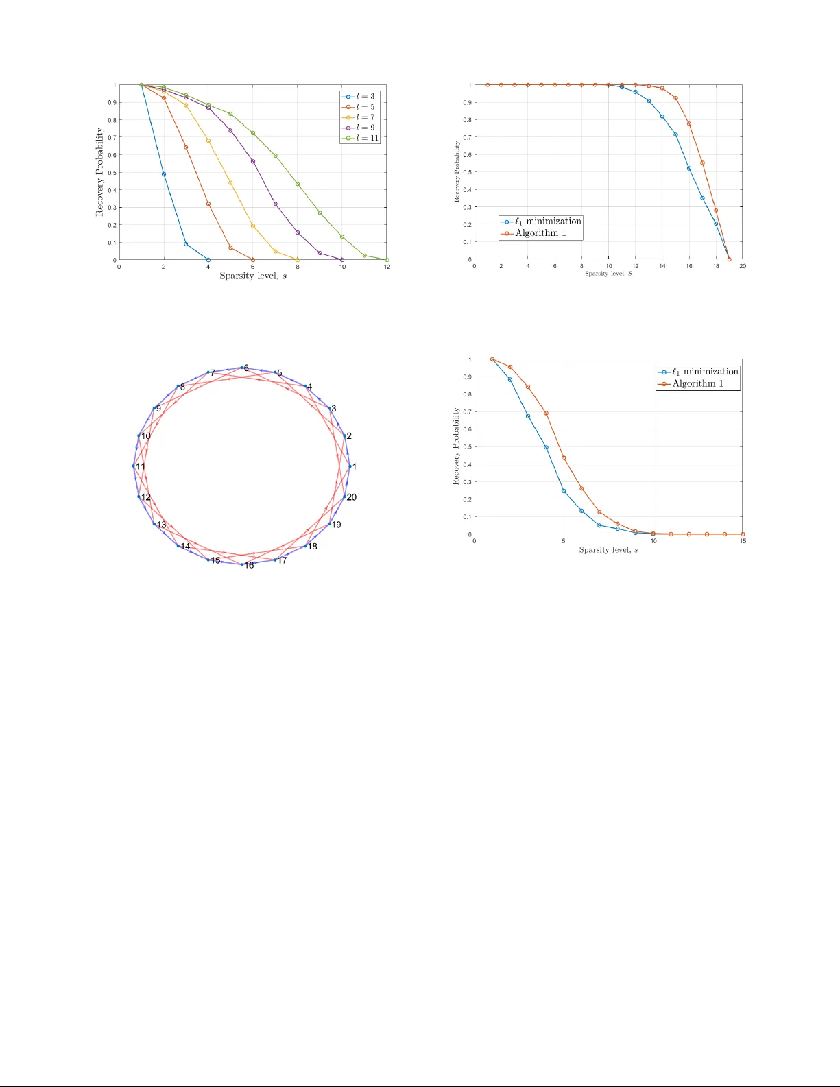
Sparse Recov ery ov er Graph Incidence Matrices Mengnan Zhao, M. De vrim Kaba, Ren ´ e V idal, Daniel P . Robinson, and Enrique Mallada Abstract — Classical results in sparse r ecovery guarantee the exact reconstruction of s -sparse signals under assumptions on the dictionary that are either too str ong or NP-hard to check. Moreo ver , such results may be pessimistic in practice since they are based on a worst-case analysis. In this paper , we consider the sparse recovery of signals defined over a graph, f or which the dictionary takes the form of an incidence matrix. W e derive necessary and sufficient conditions f or sparse reco very , which depend on properties of the cycles of the graph that can be checked in polynomial time. W e also derive support-dependent conditions for sparse recovery that depend only on the intersection of the cycles of the graph with the support of the signal. Finally , we exploit sparsity properties on the measurements and the structure of incidence matrices to propose a specialized sub-graph-based recovery algorithm that outperforms the standard ` 1 -minimization approach. I . I N T RO D U C T I O N Recently , sparse recovery methods (e.g. see [1], [2]) hav e become very popular for compressing and processing high- dimensional data. In particular, they ha ve found widespread applications in data acquisition [3], machine learning [4], [5], medical imaging [6]–[9], and networking [10]–[12]. The goal of sparse recovery is to reconstruct a signal ¯ x ∈ R n from m < n linear measurements y = Φ ¯ x ∈ R m , where Φ ∈ R m × n is the measurement matrix (also known as dictionary or sparsifying basis). In general, the reco very problem is ill-posed unless ¯ x is assumed to satisfy additional assumptions. For example, if we assume that ¯ x is s -sparse 1 , where s  n , then mild conditions on the measurement matrix Φ (see Lemma 1) allow for the reco very ¯ x from y using the ` 0 -minimization problem min x k x k 0 s.t. y = Φ x, (1) where k x k 0 denotes the number of nonzero entries in x . Howe ver , problem (1) is known to be NP-hard [13]. T o address this challenge, a common strategy is to solve a con ve x relaxation of (1) based on ` 1 -minimization given by min x k x k 1 s.t. y = Φ x, (2) which can be written equiv alently as a linear program. It is kno wn that the sparse signal can be recov ered from (2) if the measurement matrix Φ satisfies certain conditions. In general, these conditions are either computationally hard to M. Zhao and E. Mallada are with the Department of Electrical and Computer Engineering, M.D. Kaba and D.P . Robinson are with the De- partment of Applied Mathematics and Statistics, and R. V idal is with the Department of Biomedical Engineering, at The Johns Hopkins Uni- versity , Baltimore, MD 21218, USA. Emails: { mzhao21, mkaba1, rvidal, daniel.p.robinson, mallada } @jhu.edu This work was supported by NSF grants 1618637 and AMPS 1736448. 1 The vector ¯ x is s -sparse if and only if at most s of its entries are nonzero. verify , or too conservati ve so that false negativ e certificates are often encountered. For example, the Nullspace Prop- erty (NUP) [14], which provides necessary and sufficient conditions for sparse recov ery , and the Restricted Isometry Pr operty (RIP) [15], [16], which is only a suf ficient condition for sparse recov ery , are both NP-hard [17] to check. On the other hand, the Mutual Coher ence [18] property is a sufficient condition that can be efficiently verified [17], but is conserv ativ e in that it fails to certify that sparse recovery is possible for many measurement matrices seen in practice. Another major limitation of these recov ery guarantees and their associated computational complexity arises because they must allow for the worst case problem in their deriv a- tion. For e xample, the fact that the NUP and RIP are NP-hard to check does not prohibit efficient verification for particular subclasses of matrices. Similarly , ev en when the NUP is not satisfied for a sparsity le vel s , it may still be possible to recover certain subsets of s -sparse signals by exploiting additional kno wledge about their support. These observ ations suggest studying the sparse recovery problem for subclasses of matrices and signals to obtain conditions that are easier to verify as well as specialized algorithms with improv ed recov ery performance. The goal of this paper is to study sparse recovery of signals that are defined ov er graphs when the measurement matrix is the graph’ s incidence matrix. Our interest in incidence matrices stems from the fact that they are a fundamental representation of graphs, and thus a natural choice for the dictionary when analyzing network flows. In various appli- cation areas like communication networks, social networks, and transportation networks, the incidence matrices naturally appear when modeling the flow of information, disease, and goods (e.g., the detection of sparse structural network changes via observations at the nodes can be modeled as (1), where the incidence matrix serves as a measurement matrix). The main contributions of this paper are as follo ws: 1) W e derive a topological characterization of the NUP for incidence matrices. Specifically , we show that the NUP for these matrices is equiv alent to a condition on simple cycles of the graph, which is a finite subset of the nullspace of the incidence matrix. As a conse- quence, we show that for incidence matrices the sparse recov ery guarantee depends only on the girth 2 of the underlying graph. This overcomes NP-hardness, as the girth of a graph can be calculated in polynomial time. 2) Using the abo ve topological characterization, we fur- ther deriv e necessary and suf ficient conditions on the 2 Girth: Size of the smallest cycle. support of the sparse signal that enable its recov ery . Specifically , for incidence matrices we show that all signals with a given support can be recovered via (2) if and only if the support consists of strictly less than half of the edges in ev ery simple cycle of the graph. Since our conditions on ¯ x depend on its support, we will refer to them as support-dependent conditions. 3) W e propose a specialized algorithm that utilizes the knowledge of the support of the measurements and the structure of incidence matrices to constrain the support of the signal ¯ x , and consequently can guarantee sparse recov ery of ¯ x under even weaker conditions. The remainder of this paper is organized as follows: In Section II we re view basic concepts from con vex analysis, graph theory , and sparse recov ery . In Section III we formulate sparse reco very problem for incidence matrices, deriv e condi- tions for sparse and support-dependent recov ery , and propose an efficient algorithm to solve the problem. In Section IV we present numerical experiments that illustrate our theoretical results, and in Section V we provide some conclusions. I I . P R E L I M I NA R I E S A. Notation Giv en x ∈ R n , we let k x k p for p ≥ 1 denote the ` p -norm, and denote the function that counts the number of nonzero entries in x by k x k 0 . Although, the latter function is not a norm, we follo w the common practice of calling it the ` 0 - norm. For p ≥ 1 , we define the unit ` p -sphere in R n as S n − 1 p := { x ∈ R n : k x k p = 1 } . Similarly , the unit ` p -ball in R n is defined as B n p := { x ∈ R n : k x k p ≤ 1 } . The nullspace of a matrix Φ will be denoted by Null(Φ) . As usual, | S | denotes the cardinality of a set S . For a vector x ∈ R n and a nonempty inde x set S ⊆ { 1 , . . . , n } , we denote the subvector of x that corresponds to S by x S , and the associated mapping by Γ S : R n → R | S | , i.e., x S := Γ S ( x ) . The complement of S in { 1 , . . . , n } is denoted by S c . B. Con vex analysis Critical to our analysis will be the notion of e xtreme points of a con vex set and of quasi-conv ex functions. Definition 1: An extr eme point of a conv ex set C ⊂ R n is a point in C that cannot be written as a conv ex combination of two different points from C . The set of all extreme points of a con vex set C ⊂ R n is denoted by Ext( C ) . Definition 2: Let C ⊆ R n be a con ve x set. A function f : C → R is called quasi-conve x if and only if for all x, y ∈ C and λ ∈ [0 , 1] it holds that f ( λx + (1 − λ ) y ) ≤ max { f ( x ) , f ( y ) } . (3) It is easy to sho w that a function f : C → R is quasi- con ve x if and only if every sublevel set S α := { x ∈ C | f ( x ) ≤ α } is a con vex set. Every con vex function is quasi-con ve x. In particular , ` p -norm functions for p ≥ 1 are quasi-con ve x. The next result on quasi-conv ex functions [19] is included for completeness. Pr oposition 1: Let C ⊂ R n be a compact con ve x set and f : C → R be a continuous quasi-con ve x function. Then f attains its maximum v alue at an extreme point of C . C. Graph theory A directed graph with v ertex set V = { v 1 , . . . , v m } and edge set E = { e 1 , . . . , e n } ⊆ V × V will be denoted by G ( V , E ) . When the edge and verte x sets are irrelev ant to the discussion, we will drop them from the notation and denote the graph by G . Sometimes the verte x set and the edge set of G will be denoted by V ( G ) and E ( G ) respecti vely . A graph G is called simple if there is at most one edge connecting any two vertices and no edge starts and ends at the same verte x, i.e. G has no self loops. Henceforth, G will alw ays denote a simple directed graph with a finite number of edges and vertices. Although we focus on directed graphs, our analysis only requires the undirected variants of the definitions for paths, cycles, and connectivity . W e say that two vertices { a, b } ⊆ V are adjacent if either ( a, b ) ∈ E or ( b, a ) ∈ E . A sequence ( u 1 , . . . , u r ) of distinct vertices of a graph G such that u i and u i +1 are adjacent for all i ∈ { 1 , . . . , r − 1 } is called a path . A connected component ˆ G of G is a subgraph of G in which any two distinct vertices are connected to each other by a path and no edge exists between V ( ˆ G ) and V ( G ) \ V ( ˆ G ) . W e will say that the graph G is connected (for directed graphs this is often referred to as weakly connected) if G has a unique connected component. A sequence ( u 1 , . . . , u r , u 1 ) of adjacent vertices of a graph G is called a (simple) cycle if r ≥ 3 and u i 6 = u j whenev er i 6 = j ; the length of such a cycle is r . The length of the shortest simple cycle of a graph G is called the girth of G . For an acyclic graph (i.e., a graph with no cycles), the girth is defined to be + ∞ . Since acyclic graphs are not interesting for our purposes, we will assume that the girth is finite. That is, the graph has at least one simple cycle. Associated with a directed graph G = G ( V , E ) , we can define the incidence matrix A = A ( G ) ∈ R m × n as a ij =      − 1 , if v i is the initial verte x of edge e j , 1 , if v i is the terminal verte x of edge e j , 0 , otherwise. (4) For a nonempty index set S ⊆ { 1 , . . . , n } , the subgraph of G consisting of edges { e j | j ∈ S } is denoted by G S . The incidence matrix of G S is denoted by A S . Let C = ( u 1 , . . . , u r , u r +1 = u 1 ) be a simple cycle of a simple directed graph G . Then, C can be associated with a vector w ( C ) ∈ R n , where each coordinate w j of w ( C ) is defined as w j =      1 , if e j = ( u i , u i +1 ) for some i ∈ { 1 , . . . , r } − 1 , if e j = ( u i +1 , u i ) for some i ∈ { 1 , . . . , r } 0 , otherwise. (5) W e now define the cycle space of G as the subspace spanned by { w ( C ) | C is a simple cycle of G } . 3 Remark 1: The cycle space of G is exactly the nullspace of the incidence matrix A ( G ) [20]. Remark 2: The dimension of the nullspace of A ( G ) is n − m + k , where k is the number of connected components of G . Hence, the rank of A ( G ) is m − k [20]. 3 Sometimes this subspace is called the Flow Space [20]. 8 9   8   1 1 / / 4   2 2   7 4 3 3 o o 5 / / 5 6 / / 6 7 O O 9 10 o o Fig. 1: A connected directed simple graph. Example 1: The incidence matrix of the graph in Fig. 1 is gi ven by A =               − 1 0 0 − 1 0 0 0 0 0 0 1 − 1 0 0 0 0 0 0 1 0 0 1 − 1 0 − 1 0 0 0 0 0 0 0 1 1 0 0 0 0 0 0 0 0 0 0 1 − 1 0 0 0 0 0 0 0 0 0 1 − 1 0 0 1 0 0 0 0 0 0 1 1 0 0 0 0 0 0 0 0 0 − 1 − 1 0 0 0 0 0 0 0 0 0 0 − 1               , and the vectors from (5) associated with the simple cycles C 1 = (1 , 2 , 3 , 4 , 1) , C 2 = (2 , 3 , 5 , 6 , 7 , 8 , 2) , C 3 = (1 , 2 , 8 , 7 , 6 , 5 , 3 , 4 , 1) are gi ven by w 1 =  1 1 1 − 1 0 0 0 0 0 0  T w 2 =  0 1 0 0 1 1 1 − 1 1 0  T w 3 =  1 0 1 − 1 − 1 − 1 − 1 1 − 1 0  T . Note that w 3 = w 1 − w 2 , so that Null( A ( G )) must be of dimension 2 . The addition/subtraction operations on w j ’ s correspond to “addition/subtraction” operations on edges. D. Sparse Recovery It is known [21] that ev ery vector ¯ x ∈ R n with supp( ¯ x ) ⊆ S is the unique solution to (2) if and only if k η S k 1 < k η S c k 1 for all η ∈ Null(Φ) \ { 0 } . (6) This leads us to the definition of the Nullspace Pr operty . Definition 3 (Nullspace Pr operty , NUP): A matrix Φ ∈ R m × n is said to satisfy the nullspace pr operty (NUP) of order s , if for any η ∈ Null(Φ) \ { 0 } , and any nonempty index set S ⊆ { 1 , . . . , n } with | S | ≤ s , we have k η S k 1 < k η S c k 1 . Another needed concept is the spark of a matrix. Definition 4 (Spark): The spark of a matrix Φ ∈ R m × n is the smallest number of linearly dependent columns in Φ . Formally , we have spark(Φ) := min η 6 =0 k η k 0 s.t. Φ η = 0 . W e note that the rank of a matrix may be used to bound its spark. Specifically , it holds that spark(Φ) ≤ rank(Φ) + 1 . (7) The spark may be used to provide a necessary and suf ficient condition for uniqueness of sparse solutions [21]. Lemma 1: For any matrix Φ ∈ R m × n , the s -sparse signal ¯ x ∈ R n is the unique solution to the optimization problem min Φ ¯ x =Φ x k x k 0 (8) if and only if spark(Φ) > 2 s . I I I . M A I N R E S U LT S It is not dif ficult to prove that the spark of an incidence matrix A is equal to the girth of the underlying graph G . By combining this fact with Lemma 1, we obtain the following. Pr oposition 2: Let A = A ( G ) ∈ R m × n be the incidence matrix of a simple, connected graph G with girth g . Then, for ev ery s -sparse vector ¯ x ∈ R n , ¯ x is the unique solution to min A ¯ x = Ax k x k 0 (9) if and only if s < g 2 . Even though Proposition 2 is useful as a uniqueness result, it does not come in handy when one would like to recov er the original signal ¯ x from the measurements A ¯ x . For this purpose, an ` 1 -relaxation of the optimization problem is preferable. Hence, one needs a theorem akin to Proposition 2 that addresses the solutions of the optimization problem min A ¯ x = Ax k x k 1 . (10) This leads us to study the NUP for incidence matrices. Specifically , in this section we answer the following ques- tions about the incidence matrix A ∈ R m × n of a simple connected graph G with n edges and m vertices, and an s -sparse vector ¯ x ∈ R n : 1) What are necessary and sufficient conditions for A to satisfy the NUP of order s ? Such conditions would guarantee sparse recov ery , i.e., that any s -sparse signal ¯ x can be recov ered as the unique solution to (10). 2) If traditional sparse reco very is not possible, can we characterize subclasses of sparse signals that are recov- erable via (10) in terms of the support of the signal and the topology of the graph G ( V , E ) ? 3) Can we use the support of the measurement A ¯ x and the structure of A to deri ve constraints on the support of ¯ x that allow us to modify (10) and successfully recover the sparse signal ¯ x ? A. T opological Characterization of the Nullspace Pr operty for the Class of Incidence Matrices Before addressing the questions abov e in detail, we would like to build a simple framework to study them. W e will start with a reformulation of the NUP . Lemma 2: A matrix Φ ∈ R m × n satisfies the NUP of order s if and only if max | S |≤ s max η ∈ Null(Φ) ∩ B n 1 k η S k 1 < 1 2 . (11) Pr oof: For η ∈ Null(Φ) \ { 0 } , using k η k 1 = k η S k 1 + k η S c k 1 , we get k η S k 1 < k η S c k 1 if and only if k η S k 1 k η k 1 < 1 2 . Using this inequality and Definition 3, it follows that Φ satisfies NUP of order s if and only if max | S |≤ s sup η ∈ Null(Φ) \{ 0 } k η S k 1 k η k 1 < 1 2 . (12) Since the objectiv e function in (12) is independent of the scale of η , the condition in (12) is equiv alent to max | S |≤ s max η ∈ Null(Φ) ∩ S n − 1 1 k η S k 1 < 1 2 . (13) Since we can replace S n − 1 1 with B n 1 (this does not change the result of the maximization problem), we find that (13) is equiv alent to (11), as claimed. Remark 3: The value of the left hand side of (11) is called the nullspace constant in the literature [17]. The calculation of the nullspace constant for an arbitrary matrix Φ and sparsity s is kno wn to be NP-hard [17]. The reformulation of the NUP in Lemma 2 has certain benefits. For a fixed index set S ⊆ { 1 , . . . , n } , it draws our attention to the optimization problem max η ∈ Null(Φ) ∩ B n 1 k η S k 1 (14) which is the maximization of a continuous con vex function k Γ S ( · ) k 1 ov er a compact con ve x set Null(Φ) ∩ B n 1 . Thus, it follows from Proposition 1 that the maximum is attained at an extreme point of Null(Φ) ∩ B n 1 . This leads us to want to understand the extreme points of this set, which can be a computationally in volv ed task for arbitrary matrices Φ . Nonetheless, one can still set a bound on the sparsity of the extreme points of Null(Φ) ∩ B n 1 . Lemma 3: If Φ ∈ R m × n is an m × n matrix of rank r , then extreme points of Null(Φ) ∩ B n 1 are at most ( r + 1) -sparse. Pr oof: If dim(Null(Φ)) ≡ n − r ≤ 1 , then the result of the lemma holds trivially since r + 1 ≥ n . The unit ` 1 -sphere in R n , namely S n − 1 1 , may be written as the union of ( n − 1) -dimensional simplices. Hence, if dim(Null(Φ)) ≡ n − r ≥ 1 , each extreme point is contained in an ( n − 1) -dimensional simplex. In particular , if dim(Null(Φ)) ≡ n − r > 1 , we argue that, no extreme point of Null(Φ) ∩ B n 1 lies in the interior of these ( n − 1) -dimensional simplices. This is because in this case the intersection of Null(Φ) and the interior of the ( n − 1) -dimensional simplex is either empty , or a non- singleton open con vex subset of R n , where e very point is a con ve x combination of two distinct points. Hence, no extreme point can live there. So, the extreme points must lie in the boundary of ( n − 1) -dimensional simplices, which are ( n − 2) -dimensional simplices. Moreover , these ( n − 2) - dimensional simplices are where one coordinate becomes zero. Hence, at least one coordinate of an extreme point living in an ( n − 2) -dimensional simplex is zero. As long as the sum of the dimension of the simplex, which contains the extreme point, and the dimension of Null(Φ) is strictly larger than n , we could repeat the argument in the previous paragraph. This ar gument stops when the dimension of the simplex containing the extreme point is r . Thus, at least n − r − 1 coordinates of the extreme point have to be zero, so that each extreme point is at most ( r + 1) -sparse. Although Lemma 3 is analogous to (7), it is stronger in the sense that the statement bounds the sparsity of all the extreme points of the con ve x set Null(Φ) ∩ B n 1 , not just the sparsest vectors in the Null(Φ) , as is implied by (7). Armed with Lemma 3, it turns out that for incidence matrices, these extreme points ha ve a nice characterization in terms of the properties of the underlying graph. Pr oposition 3: Let A ∈ R m × n be the incidence matrix of a simple connected graph G that has at least one simple cycle, and let W 1 denote the set of normalized simple cycles of G , i.e. W 1 :=  w ( C ) k w ( C ) k 1 | C is a simple cycle of G  . (15) Then, we hav e Ext(Null( A ) ∩ B n 1 ) ⊆ W 1 . Pr oof: Let z be an extreme point of Null( A ) ∩ B n 1 with support S . W e necessarily hav e k z k 1 = 1 . Suppose that G S has ¯ m vertices and ¯ k connected components. Note that z S ∈ Null( A S ) ∩ B | S | 1 has only nonzero entries. W e claim that z S is an e xtreme point of Null( A S ) ∩ B | S | 1 . For a proof by contradiction, suppose that z S could be written as a con ve x combination of two distinct vectors in Null( A S ) ∩ B | S | 1 . In this case, one could pad those vectors with zeros at the coordinates in S c to get two distinct vectors in Null( A ) ∩ B n 1 , whose con ve x combination would gi ve z . Since this would contradict the fact that z is an extreme point, we must conclude that z S is an extreme point of Null( A S ) ∩ B | S | 1 . Using the fact that z S is an extreme point of Null( A S ) ∩ B | S | 1 , Lemma 3, and Remark 2, it follows that | S | ≤ rank( A S ) + 1 = ¯ m − ¯ k + 1 . (16) Combining (16) with the rank-nullity theorem yields dim(Null( A S )) = | S | − ¯ m + ¯ k ≤ 1 . This may be combined with 0 6 = z S ∈ Null( A S ) to conclude that dim(Null( A S )) = 1 ; thus Null( A S ) is spanned by z S . It now follo ws from Remark 1 that z S corresponds to the unique simple cycle in G S . In addition, since z S has no zero entries, the corresponding simple cycle includes e very edge of G S . It follows that z corresponds to a simple cycle in G , which combined with k z k 1 = 1 prov es z ∈ W 1 . Next we show that Proposition 3 provides a way to study the maximization problem (14). Theor em 1: Let A ∈ R m × n be the incidence matrix of a simple, connected graph G , and let W 1 denote the set of normalized simple cycles of G as in (15). Let S ⊆ { 1 , . . . , n } be a nonempty index set. Then max η ∈ Null( A ) ∩ B n 1 k η S k 1 = max z ∈ W 1 k z S k 1 . (17) Pr oof: Since W 1 ⊂ Null( A ) ∩ B n 1 , we obviously have max η ∈ Null( A ) ∩ B n 1 k η S k 1 ≥ max z ∈ W 1 k z S k 1 . For the conv erse inequality we argue as follows: Since k Γ S ( · ) k 1 is a continuous con vex function (thus also quasi- con ve x), and Null( A ) ∩ B n 1 is a compact con ve x set, the maximum in the left hand side of (17) will be attained at an extreme point of Null( A ) ∩ B n 1 (see Proposition 1). That is, max η ∈ Null( A ) ∩ B n 1 k η S k 1 = max ν ∈ Ext(Null( A ) ∩ B n 1 ) k ν S k 1 . (18) But Ext(Null( A ) ∩ B n 1 ) ⊆ W 1 by Proposition 3. Hence, max ν ∈ Ext(Null( A ) ∩ B n 1 ) k ν S k 1 ≤ max z ∈ W 1 k z S k 1 . Combining this with (18) we get the conv erse inequality , and hence the result. Theorem 1 builds a connection between the algebraic condition NUP and a topological property of the graph, namely its simple cycles. This connection is what we will primarily exploit in the rest of the paper . Let us make a simple but important observation. Lemma 4: Let G and W 1 be as in Theorem 1. Then, for any index set S and z ∈ W 1 , it holds that k z S k 1 = | S ∩ supp( z ) | k z k 0 . Pr oof: For any simple cycle C , the entries of w ( C ) are in the set { 0 , − 1 , 1 } . Hence, entries of any z ∈ W 1 are from the set { 0 , 1 k z k 0 , − 1 k z k 0 } , from which the result follows. B. P olynomial T ime Guarantees for Sparse Recovery An answer to the first question posed at the beginning of Section III is gi ven by Theorem 2. Theor em 2: Let A ∈ R m × n be the incidence matrix of a simple, connected graph G with girth g . Then, e very s -sparse vector ¯ x ∈ R n is the unique solution to min A ¯ x = Ax k x k 1 if and only if s < g 2 . Pr oof: From Lemma 2 and Theorem 1 it follo ws that the NUP of order s is satisfied if and only if max | S |≤ s max z ∈ W 1 k z S k 1 < 1 2 . (19) From Lemma 4, the maximum on the left of (19) is equal to max | S |≤ s max z ∈ W 1 | S ∩ supp( z ) | k z k 0 . (20) If s ≥ g , then (20) is equal to 1 . If s < g , the maximum is attained at the smallest simple cycle when S picks edges only from this cycle, and the maximum is equal to s g . Hence, max | S |≤ s max z ∈ W 1 k z S k 1 = min { s/g , 1 } . (21) The desired result no w follo ws from (19) and (21). Remark 4: As was mentioned in Remark 3, calculating the nullspace constant is NP-hard in general. Howe ver , there are algorithms that can calculate the girth of a graph exactly in O ( mn ) or sufficiently accurately for our purposes in O ( m 2 ) (see [22]). Therefore, Theorem 2 rev eals that the nullspace constant can be calculated—hence the NUP can be verified—for graph incidence matrices in polynomial time. C. Guarantees for Support-dependent Sparse Recovery The sparse recov ery result giv en by Theorem 2 depends on the cardinality s of the support of the unknown signal. For a graph with small girth (e.g., g = 3 ), this result establishes sparse recov ery guarantees only for signals with low sparsity lev els (specifically , s < g / 2 ). It is natural, therefore, to ask the following question: Given a graph with relativ ely small girth, can we identify a class of signals with sparsity s ≥ g / 2 that can be recovered? This leads us to the study of support- dependent sparse recovery , where we not only focus on the cardinality of the support of the unkno wn signal ¯ x , but also take the location of the support into account. More precisely , we hav e the following result. Theor em 3: Let A ∈ R m × n be the incidence matrix of a simple, connected graph G , let W 1 denote the set of normalized simple cycles of G as in (15), and let ∅ 6 = S ⊆ { 1 , . . . , n } . Then, ev ery vector ¯ x ∈ R n with supp( ¯ x ) ⊆ S is the unique solution to the optimization problem min A ¯ x = Ax k x k 1 (22) if and only if max z ∈ W 1 | S ∩ supp( z ) | k z k 0 < 1 2 . (23) Pr oof: From arguments in the proof of Lemma 2, we know that (6) is equi valent to max η ∈ Null( A ) ∩ B n 1 k η S k 1 < 1 2 , which with Theorem 1 and Lemma 4 gives the result. Remark 5: In comparison to Theorem 2, Theorem 3 pro- vides a deeper insight into the vectors ¯ x that can be recov ered from the observations A ¯ x via ` 1 -minimization. Specifically , any vector whose support within each simple cycle has size strictly less than half the size of that cycle, can be successfully recov ered. As an example consider the graph in Fig. 1, which has girth g = 4 . Thus, it follo ws from Theorem 2 that any 1 - sparse signal can be recov ered. Howe ver , in reality , some signals that are supported on more than one edge can also be recov ered. For instance, Theorem 3 guarantees that a signal ¯ x supported on edges { 2 , 7 } or { 4 , 6 , 8 } can be reco vered as the unique solution to the ` 1 problem (22) since for each of the three simple cycles, its intersection with the support of the unknown v ector ¯ x is less than half of the length of the simple cycle. This rev eals that different sparsity patterns of the same sparsity le vel can have different recovery performances. Remark 6: T o use Theorem 3 as a way of providing a support-dependent recovery guarantee, one needs to compute the intersection of the support of ¯ x with all simple cycles in the graph. A number of algorithms with a polynomial time complexity bound for cycle enumeration are known [23]. D. Using Measurement Sparsity to Aid Recovery When there is additional information about the support of the unknown signal, Theorem 3 giv es a necessary and sufficient condition for exact reco very . In practice, this in- formation is usually missing. Ho wev er , the special structure of the incidence matrix and its connection to the graph can help us circumvent this difficulty . Notice that the columns of any incidence matrix are always 2 -sparse, which means that the measurement y := A ¯ x will be 2 s -sparse for any s -sparse signal ¯ x . Therefore, one can seek to obtain a superset of supp( ¯ x ) by observing supp( y ) , i.e. the vertices with nonzero measurements. T ypically , this observation reduces the size of the problem, and gi ves rise to Algorithm 1. Algorithm 1 Recovering the unknown signal by using sparse verte x measurements. 1: INPUT : y ∈ R m , A ∈ R m × n , G ( V , E ) . 2: Set ˆ x = 0 . 3: Define T := supp( y ) . 4: Define S := { j | e j = ( v i , v k ) ∈ E and v i , v k ∈ T } , the indices of the edges of G connecting vertices with nonzero measurements. 5: Construct G S , the subgraph of G consisting of the edges index ed by S . 6: Construct the incidence matrix A S of the subgraph G S . 7: Solve the ` 1 -minimization problem ˜ x = arg min y T = A S x k x k 1 8: Set ˆ x S = ˜ x . 9: return ˆ x ∈ R n Remark 7: There are cases where Algorithm 1 may fail. For instance, when the unknown nonzero signal ¯ x is in the nullspace of one of the rows of A , say a k , and supp( a k ) ∩ supp( ¯ x ) 6 = ∅ (i.e. when the non-zero values of the signal ¯ x cancel each other at a verte x k ), Algorithm 1 would simply ignore the corresponding verte x, and hence, the edges connected to it. This leads to a wrong subgraph G S and possibly an incorrect outcome ˆ x . Fortunately , this case happens with zero probability when the signal has random support and random v alues. Cor ollary 1: Let A ∈ R m × n be the incidence matrix of a simple, connected graph G . Gi ven a random signal ¯ x , let y := A ¯ x and G S be the subgraph associated with y in Algorithm 1. Then, Algorithm 1 will almost surely recover the signal ¯ x if and only if supp( ¯ x ) picks strictly less than half of the edges from each simple cycle of G S . The proof of Corollary 1 follows from Theorem 3 and the fact that ¯ x is assumed to be randomly generated. In comparison to ` 1 -minimization on the original graph, Algorithm 1 may have improv ed support-dependent recov ery performance because the formation of the subgraph may eliminate cycles; this is especially true for large-scale net- works. For concreteness, let us gi ve a simple example. Example 2: Consider the graph depicted in Fig. 1. Let ¯ x be a random signal that is supported on the edges 8 8   1 4   7 4 3 3 o o 5 / / 5 6 / / 6 7 O O 9 10 o o Fig. 2: Acyclic subgraph G S induced by an unknown signal with support S = { 3 , 4 , 5 , 6 , 7 , 8 , 10 } . { 3 , 4 , 5 , 6 , 7 , 8 , 10 } , so that (with probability one) there are nonzero measurements on nodes { 1 , 3 , 4 , 5 , 6 , 7 , 8 , 9 } . Then, x cannot be recov ered using the incidence matrix of the orig- inal graph. Howe ver , the subgraph G S is acyclic, as shown in Fig. 2, which allows exact recovery via Algorithm 1. I V . S I M U L A T I O N S In this section we provide numerical simulation results on the recov ery performance associated with incidence matrices. In all experiments, the signal ¯ x has random support with each nonzero entry drawn i.i.d. from the standard normal distribution. W e use the CVX software package [24] to solve the optimization problems. A vector is declared to be recov ered if the 2 -norm error is less than or equal to 10 − 5 . Experiment 1: Fig. 4 shows the probability of exact re- cov ery of signals via ` 1 -relaxation over a sequence of graphs containing two cycles (see Fig. 3). Each graph has a cycle of length 3 and a larger one of varying lengths 3 , 5 , 7 , 9 , and 11 , respectiv ely . For each sparsity lev el, 1000 trials were performed. According to Theorem 2, for all graphs we can recov er 1-sparse signals since the girth is 3 for each graph in the sequence. When the sparsity le vel is increased, we expect that the probability of exact recovery will increase for graphs with larger cycles because it becomes less likely that the support of the random signal will consist of more than half of the edges for one of the simple cycles in the graph. Note that this agrees with our observation in Fig. 4. Experiment 2: W e no w ev aluate the performance of Al- gorithm 1 against the ` 1 -minimization method in (10) on 2     3 $ $ 1 g g l + 1 E E Fig. 3: Graph used in Experiment 1, which consists of a c ycle of length 3 and a cycle of varying length l ∈ { 3 , 5 , 7 , 9 , 11 } . Fig. 4: Probability of exact recovery as a function of the sparsity le vel for the graphs of various loop sizes in Fig. 3. Fig. 5: Graphs with 20 nodes for Experiment 2. G B consists of blue edges only and G B R consists of blue and red edges. two graphs with 20 nodes (see Fig. 5). The first graph, G B , is a simple cycle connecting node 1 to node 20 in order (blue edges in Fig. 5). The second graph, G B R , consists of both blue and red edges. The red edges connect each node to its third neighbor, i.e., (1 , 4) , (2 , 5) · · · (17 , 20) · · · (20 , 3) . Fig. 6 and Fig. 7 sho w the performance of both algorithms on G B and G B R respectiv ely . For each sparsity lev el, the experiments are repeated 1000 times to compute recov- ery probabilities. For G B , Algorithm 1 outperforms ` 1 - minimization since the reduced graph in Algorithm 1 will be acyclic in some cases. For G B R , Algorithm 1 will eliminate small cycles when forming the subgraph and lead to higher recov ery probability for fixed s due to a larger girth. V . C O N C L U S I O N In this paper we studied sparse recovery for the class of graph incidence matrices. For such matrices we provided a characterization of the NUP in terms of the topological prop- erties of the underlying graph. This characterization allows one to verify sparse recovery guarantees in polynomial time for the class of incidence matrices. Moreover , we showed Fig. 6: Probability of exact recovery as a function of the sparsity le vel for Algorithm 1 and ` 1 -minimization on G B . Fig. 7: Probability of exact recovery as a function of the sparsity lev el for Algorithm 1 and ` 1 -minimization on G B R . that support-dependent recov ery performance can also be analyzed in terms of the simple cycles of the graph. Finally , by exploiting the structure of incidence matrices and sparsity of the measurements, we proposed an efficient algorithm for recov ery and e valuated its performance numerically . R E F E R E N C E S [1] D. L. Donoho, “Compressed sensing, ” IEEE T ransactions on Infor- mation Theory , vol. 52, no. 4, pp. 1289–1306, 2006. [2] S. Mallat, A wavelet tour of signal processing: the sparse way . Academic press, 2008. [3] E. J. Cand ` es and M. B. W akin, “ An introduction to compressive sampling, ” IEEE Signal Pr ocessing Magazine , vol. 25, no. 2, pp. 21– 30, 2008. [4] E. Elhamifar and R. V idal, “Sparse subspace clustering, ” in IEEE Confer ence on Computer V ision and P attern Recognition , pp. 2790– 2797, IEEE, 2009. [5] J. Wright, A. Y . Y ang, A. Ganesh, S. S. Sastry , and Y . Ma, “Rob ust f ace recognition via sparse representation, ” IEEE T ransactions on P attern Analysis and Machine Intelligence , vol. 31, no. 2, pp. 210–227, 2009. [6] M. Lustig, D. Donoho, and J. Pauly , “Rapid MR imaging with compressed sensing and randomly under-sampled 3DFT trajectories, ” in Pr oc. 14th Ann. Meeting ISMRM , Citeseer, 2006. [7] M. Lustig, D. Donoho, and J. M. Pauly , “Sparse MRI: The application of compressed sensing for rapid MR imaging, ” Magnetic Resonance in Medicine , vol. 58, no. 6, pp. 1182–1195, 2007. [8] E. J. Cand ` es, J. Romberg, and T . T ao, “Robust uncertainty principles: Exact signal reconstruction from highly incomplete frequency infor- mation, ” IEEE T ransactions on Information Theory , vol. 52, no. 2, pp. 489–509, 2006. [9] R. Li ´ egeois, B. Mishra, M. Zorzi, and R. Sepulchre, “Sparse plus low-rank autoregressiv e identification in neuroimaging time series, ” in IEEE Confer ence on Decision and Contr ol , pp. 3965–3970, 2015. [10] M. Coates, Y . Pointurier , and M. Rabbat, “Compressed network monitoring, ” in IEEE/SP W orkshop on Statistical Signal Pr ocessing , pp. 418–422, IEEE, 2007. [11] J. Haupt, W . U. Bajwa, M. Rabbat, and R. Nowak, “Compressed sensing for networked data, ” IEEE Signal Pr ocessing Magazine , vol. 25, no. 2, pp. 92–101, 2008. [12] W . Xu, E. Mallada, and A. T ang, “Compressiv e sensing over graphs, ” in IEEE INFOCOM , pp. 2087–2095, IEEE, 2011. [13] R. G. Michael and S. J. David, “Computers and intractability: a guide to the theory of NP-completeness, ” WH Fr ee. Co., San F r , pp. 90–91, 1979. [14] A. Cohen, W . Dahmen, and R. DeV ore, “Compressed sensing and best k -term approximation, ” Journal of the American Mathematical Society , v ol. 22, no. 1, pp. 211–231, 2009. [15] E. J. Candes and T . T ao, “Decoding by linear programming, ” IEEE T ransactions on Information Theory , vol. 51, no. 12, pp. 4203–4215, 2005. [16] R. Baraniuk, M. Davenport, R. DeV ore, and M. W akin, “ A simple proof of the restricted isometry property for random matrices, ” Con- structive Appr oximation , vol. 28, no. 3, pp. 253–263, 2008. [17] A. M. Tillmann and M. E. Pfetsch, “The computational complexity of the restricted isometry property , the nullspace property , and related concepts in compressed sensing, ” IEEE T ransactions on Information Theory , v ol. 60, no. 2, pp. 1248–1259, 2014. [18] D. L. Donoho and X. Huo, “Uncertainty principles and ideal atomic decomposition, ” IEEE T ransactions on Information Theory , vol. 47, no. 7, pp. 2845–2862, 2001. [19] F . Flores-Baz ´ an, F . Flores-Baz ´ an, and C. V era, “Maximizing and minimizing quasiconv ex functions: related properties, existence and optimality conditions via radial epideriv ativ es, ” Journal of Global Optimization , v ol. 63, pp. 99–123, Sep 2015. [20] C. Godsil and G. F . Royle, Algebraic graph theory . Graduate text in mathematics, Springer , New Y ork, 2001. [21] S. Foucart and H. Rauhut, A mathematical introduction to compr essive sensing , v ol. 1. Birkh ¨ auser Basel, 2013. [22] A. Itai and M. Rodeh, “Finding a minimum circuit in a graph, ” SIAM Journal on Computing , vol. 7, no. 4, pp. 413–423, 1978. [23] P . Mateti and N. Deo, “On algorithms for enumerating all circuits of a graph, ” SIAM Journal on Computing , vol. 5, no. 1, pp. 90–99, 1976. [24] M. Grant, S. Boyd, and Y . Y e, “CVX: Matlab software for disciplined con vex programming, ” 2008.