Deep Clustering With Intra-class Distance Constraint for Hyperspectral Images

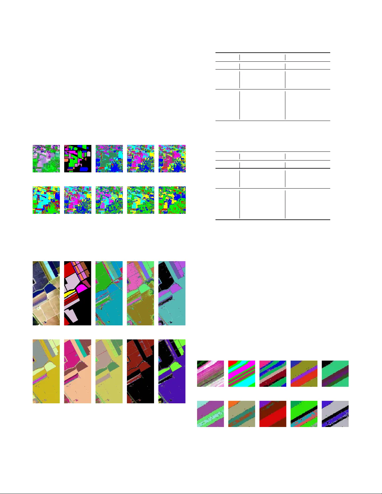
1 Deep Clustering W ith Intra-class Distance Constraint for Hyperspectral Images Jinguang Sun, W anli W ang, Xian W ei, Member , IEEE , Li Fang, Member , IEEE , Xiaoliang T ang, Y usheng Xu, Member , IEEE , Hui Y u and W ei Y ao Abstract —The high dimensionality of hyperspectral images often results in the degradation of clustering perf ormance. Due to the powerful ability of deep featur e extraction and non-linear feature representation, the clustering algorithm based on deep learning has become a hot r esearch topic in the field of h yperspec- tral r emote sensing. However , most deep clustering algorithms for h yperspectral images utilize deep neural networks as featur e extractor without considering prior knowledge constraints that are suitable for clustering. T o solve this problem, we propose an intra-class distance constrained deep clustering algorithm for high-dimensional hyperspectral images. The proposed algorithm constrains the featur e mapping procedur e of the auto-encoder network by intra-class distance so that raw images are trans- formed from the original high-dimensional space to the low- dimensional feature space that is more conducive to clustering. Furthermore, the r elated learning pr ocess is treated as a joint optimization problem of deep feature extraction and clustering. Experimental results demonstrate the intense competitiveness of the proposed algorithm in comparison with state-of-the-art clustering methods of hyperspectral images. Index T erms —Deep learning, hyperspectral images clustering, intra-class distance constraint, low-dimensional representation, remote sensing. I . I N T R O D U C T I O N W ITH the dev elopment of the remote sensing technology , a wide div ersity of sensor characteristics is nowadays av ailable. The sensing data is ranging from medium and very high resolution (VHR) multispectral images to hyperspectral images that sample the electromagnetic spectrum with high detail [1]–[8]. Utilizing these myriad sensors, the Earth Ob- servation System (EOS) generates massiv e practical images of various land covering objects. Owing to abundant spatial and spectral information, these numerous images make it possible to extend the applications of hyperspectral remote sensing to many potential fields [9]–[15]. Howe ver , it is very arduous to This work was partially supported by the Y oung Scientists Fund of the National Natural Science Foundation of China under Grant No. 61602226 and No. 61806186, and the CAS Pioneer Hundred T alents Program (T ype C) under Grant No. 2017-122. (Jinguang Sun and W anli W ang contribute equally to this work.) (Corresponding author: Xian W ei.) J. Sun and W . W ang are with the School of Electronic and Information En- gineering, Liaoning T echnical University , Huludao 125105, Liaoning, China (email: Sunjinguang@lntu.edu.cn; email: wwlswj@163.com). X. W ei, L. Fang, X. T ang and H. Y u are with the Quanzhou Institute of Equipment Manufacturing, Haixi Institute, Chinese Academy of Sciences, Quanzhou 362216, Fujian, China (email: xian.wei@fjirsm.ac.cn). Y . Xu is with the Department of Photogrammetry and Remote Sensing, T echnical University of Munich, 80333 Munich, Germany . W . Y ao is with the Department of Land Surveying and Geo-Informatics, Hong K ong Polytechnic Univ ersity , 181 Chatham Road South, Hung Hom, K owloon, Hong K ong. annotate these massiv e practical earth observation images ef- fectiv ely . Due to the lack of labeled high-dimensional samples of hyperspectral images, learning appropriate low-dimensional (LD) representations of data for clustering plays a critical role in hyperspectral image annotation and understanding. Clustering is the task of grouping a set of objects in such a way that objects in the same group are more similar to each other than to those in other groups [16]. F or remote sensing images, the task is to classify the pixels into homogeneous regions which segment ev ery image into different partitions [1], [7], [17]. Most traditional clustering algorithms are based on shallo w linear models [18]–[21], such as algorithms based on K-means [22], ISOD A T A [23] and Fuzzy C-means [4], [6], which often fail when the data exhibits an irregular non-linear distribution. During the past decades, spectral-based cluster- ing methods [5], [24]–[28] and density-based [7] clustering methods have been state-of-the-arts. Let X = [ x 1 , · · · , x n ] ∈ R m × n be the matrix containing the n independent training samples arranged as its columns, the spectral-based clustering approaches perform clustering in the following two steps. At first, an affinity matrix (i.e., similarity graph) C is built to depict the relationship of the data, where C ij denotes the similarity between data points x i and x j . Secondly , the data is clustered through clustering the eigen vectors of the graph Laplacian L = D − 1 2 AD − 1 2 , where D is a diagonal matrix with D ii = P j A ij and A = | C | +    C T    . The main idea of the density-based clustering [29] approaches are to find high-density regions that are separated by low-density regions. The density peaks clustering algorithm (DPCA) proposed by Alex Rodriguez [30] has brought the density-based clustering approaches to a new stage. The core idea of DPCA is that the centre of the cluster is surrounded by some points with lo w local density , and these points are far away from other points with high local density . The DPCA separates the clustering process of non-clustered centre points into a single process. Due to the selection of the cluster centre and the classification of the non-cluster points are separated, the clustering precision is increased. T o solve the clustering problem of more complex distrib uted data, the sparse subspace clustering (SSC) algorithm [13], [31] is dev eloped. The core idea of SSC is that among the infinite number of representations of a data point in terms of other points, a sparse representation corresponds to selecting a few points from the same subspace. In fact, the SSC algorithm is a solution of sparse optimization in the framew ork of spectral clustering, and it ev aluates the labels for e very sample in the 2 low-dimensional space. Sharing the homogeneous idea with SSC, many sparse representation and lo w-rank approximation based methods for subspace clustering [18], [32]–[35] have receiv ed a lot of attention in recent years. The key components of these methods are finding a sparse and low-rank represen- tation of the data and then building a similarity graph on the sparse coefficient matrix for the separation of the data. Although the spectral-based clustering algorithms and the density-based clustering algorithms can effecti vely cluster ar- bitrarily distributed data, only the shallow features of the data can be used [19]. Moreover , it is difficult to further improve the clustering ef fect and precision. On the other hand, deep neural networks can non-linearly map data from the original feature space to a new feature space, with the promising advantages compared with traditional clustering algorithms for deep feature extraction and dimension reduction. Therefore, in recent years, the subspace clustering algorithm based on deep learning has attracted more attention. The core idea of deep neural network clustering [36]–[40] is to non-linearly map data from the original feature space to a new feature space and then complete clustering in the new feature space. Because its mapping is non-linear , deep neural network clustering has powerful capabilities on intrin- sic feature e xtraction and data representation. The clustering algorithm based on auto-encoder netw orks [38], [41]–[43] is a popular framew ork for deep clustering algorithms, which utilizes a symmetric network structure to encode and represent the data. Such an algorithm consists of tw o important steps. Firstly , it obtains the code space of the data by reducing the data dimension and clusters the data in the obtained code space. Secondly , it performs the representation transformation from the obtained code space to a ne w generati ve feature space. Depending upon the auto-encoder network, the idea of generativ e adversarial [44]–[48] is introduced into the clustering field, which further improves the performance of deep clustering algorithms. Generally speaking, current deep clustering algorithms hav e the form [32], [42], [49], [50] as J p = J p 1 + λ    Z ( M 2 ) − Z ( M 2 ) C    2 | {z } J p 2 + J p 3 , (1) where J p is the loss function, J p 1 represents the reconstruc- tion error , J p 2 is a sparse or lo w-rank constraint determined by the pre-trained matrix C , and J p 3 is the regularization term. The λ in J p 2 represents the constraint coefficient, and Z ( M 2 ) denotes the obtained codes or extracted features by the auto- encoder . The data representation shown in (1) achiev es both data reconstruction and dimensionality reduction. Therefore, the features extracted by such algorithms are appropriate ones for data dimensionality reduction. Howe ver , due to the lack of prior knowledge constraints, the feature extraction procedure of deep clustering algorithms tends to lose some useful guides which need to be further explored. T o solve this problem, we propose an embedded deep clustering algorithm with intra- class distance constraint. The proposed algorithm embeds the global K-means model into the auto-encoder network that can constrain the procedure of data mapping and obtain data representation that is more conduciv e to clustering. The proposed algorithm has the following contributions: 1) The intra-class distance is utilized to constrain the encoding process of the auto-encoder network so that the auto-encoder network can map the data from the original feature space to the feature space which is more conduciv e to clustering. 2) The pre-training process is not necessary , and the indi- cator matrix is dynamically adjusted to image data. 3) This work treats the solution to the proposed algorithm as a joint learning optimization problem, and the entire clustering procedure is completed in one stage. I I . R E L A T E D W O R K S In this section, we briefly discuss some e xisting w orks in unsupervised deep learning and subspace clustering. A. Auto-encoder Network W ith impressive learning and characterization capabilities, auto-encoder neural networks have achiev ed great success in various areas, especially in the scenario of unsupervised learn- ing [2], [43], [51]–[53], such as natural language processing [54], image processing [55], object detection [56], biometric recognition [57], and data analysis [58]. As state-of-the-art unsupervised techniques, auto-encoder and auto-encoder based neural networks also make outstanding contrib utions in the field of remote sensing. In this subsection, we briefly introduce the auto-encoder network. In general, an auto-encoder [41] is a kind of network that consists of encoder and decoder, and the structure of the encoder and decoder is symmetrical. If the auto-encoder contains multiple hidden layers, then the number of hidden layers of the encoder is equal to the number of hidden layers of the decoder . The structural model of the basic auto-encoder is shown in Fig. 1. The purpose of the basic auto-encoder is to reconstruct the input data at the output layer , and the perfect case is that the output signal X out (i.e., Z ( M ) ) is exactly the same as the input signal X in (i.e., Z (0) ). According to the structure shown in Fig. 1, the encoding process and decoding process of the basic auto-encoder can be described as ( z ( i +1) = F e  W i z ( i ) + b i  Encoding z ( j +1) = F d  W j z ( j ) + b j  Decoding , (2) where W i , b i denote the i - th encoding weight and the i - th encoding bias, respecti vely , W j , b j represent the j - th decoding weight and the j - th decoding bias, respectively , z ( i ) denotes the data vector in i - th layer , and F e is the non-linear transformation. Sigmoid , T anh , Relu are commonly used activ ation functions for F e . F d can be the same non- linear transformation as in the encoding process. Therefore, the loss function of the basic auto-encoder is to minimize the error between X in and X out . The encoder con verts the input signal into codes through some non-linear mapping, and the decoder tries to remap the codes to the input signal. The parameters of the auto-encoder , i.e., weights and biases, are 3 learned by minimizing the total reconstruction error , which could be computed by the mean square error J m ( W , b ) = n X i =1 L  z (0) i , z ( M ) i  = n X i =1    z (0) i − z ( M ) i    2 2 , (3) or the cross entropy J c ( W , b ) = n X i =1 L  z (0) i , z ( M ) i  = − n X i =1  z (0) i log z ( M ) i +  1 − z (0) i  log  1 − z ( M ) i  . (4) For the structure shown in Fig. 1, the hidden layers of the basic automatic coding network hav e three different structures: a compressed structure, a sparse structure, and an equiv alent- dimensional structure. When the number of input layer neurons is greater than the number of hidden layer neurons, it is called a compressed structure [59]. Con versely , when the number of input layer neurons is smaller than the number of hidden layer neurons, it is called a sparse structure. If the input layer and the hidden layer have the same number of neurons, it is named the equiv alent-dimensional structure. E nc ode r D e c ode r ( 0 ) () in XZ () 2 M Z () () M out XZ Fig. 1. The structure of the auto-encoder network. B. Deep Subspace Clustering Many practical subspace clustering missions transform data from the high dimensional feature space to the lo w dimen- sional feature space. Whereas many subspace clustering algo- rithms [18], [19], [31], [35], [60], [61] are shallow models, which cannot model the non-linearity of data in practical situations. Benefiting from the powerful capabilities of non- linear modeling and data representation of the deep neural network, some clustering approaches based on deep neural networks have been proposed in recent years. Song et al. [41] integrated an auto-encoder network with K-means to cluster the latent features. Howe ver , the feature mapping and clustering are two relatively independent processes in their work, and the K-means algorithm is not jointed into the feature mapping process. Therefore, the feature mapping process may not be constrained by the K-means algorithm. With the emer- gence of generati ve adversarial networks, some deep clustering algorithms [37], [47] embedded discriminant and adversarial ideas have been proposed, which further enhance the ability of deep feature extraction and data representation. On the other hand, some deep subspace clustering algorithms with prior constraints hav e been developed. According to different constraining conditions, these prior constraints may be sparse [59], low rank [62], and least square [39]. Based on the auto-encoder network, the loss functions of these algorithms share the same modality , shown in (5). These algorithms learn representation for the input data with minimal reconstruction error and incorporate prior information into the potential feature learning to preserve the key reconstruction relation ov er the data. Although the features extracted by such algo- rithms are appropriate for the dimensionality reduction and reconstruction of the data, the procedure of feature extracting may lose the purposefulness, due to the lack of the constraints of prior knowledge. J p ( W i , b i ) = 1 2    Z (0) − Z ( M )    2 F | {z } J p 1 + λ 1 2    Z ( M 2 ) − Z ( M 2 ) C    2 F | {z } J p 2 + λ 2 2 M X i =1  k W i k 2 F + k b i k 2 2  | {z } J p 3 , (5) where J p 1 denotes the reconstruction error , J p 2 denotes the prior constraint, J p 3 denotes the re gularization term and C is a pre-trained matrix. Aforementioned deep clustering algorithms hav e following three weaknesses: 1) Lacking prior constraints related to clustering task. 2) The matrix C needs to be pre-trained, which may not be optimal for various data to be clustered. 3) Once given, the matrix C is fixed, which cannot be optimized jointly with the network. Different from these existing works, we propose an ap- proach that embeds intra-class distance into an auto-encoder network. The Indicativ e matrix and the parameters of the network are adapti vely optimized simultaneously . The pro- posed approach utilizes intra-class distance to constrain the feature mapping process of the auto-encoder so that the deep features extracted from the source space are more conduciv e for clustering. More details of the proposed approach are described in the following sections. I I I . T H E P RO P O S E D D E E P C L U S T E R I N G A P P R O A C H In this section, we elaborate on the details of the pro- posed Deep Clustering with Intra-class Distance Constraint (DCIDC) algorithm. The frame work of DCIDC is an auto- encoder network, and the specific structure may be varied according to different scenarios. W ith the constraint of intra- class distance, DCIDC extracts deep features of the data by mapping them from the source space to a latent feature space. 4 In the new latent feature space, objects in the same group are more similar to each other than to those in other groups. W e first explain how DCIDC is specifically designed and then present the algorithm for optimizing the DCIDC model. A. Deep Clustering with Intra-class Distance Constraint The neural network within DCIDC consists of M + 1 layers for performing M non-linear transformations, where M is an ev en number, the first M 2 hidden layers are encoders to learn a set of compact representations (i.e., low-dimensional repre- sentations) and the last M 2 layers are decoders to progressiv ely reconstruct the input. The framew ork of DCIDC is shown as Fig. 2. Let Z (0) = X in ∈ R N × D be one input matrix to the first layer , which denotes a hyperspectral image consisting of N image pixels (samples) and z (0) be one ro w of the matrix, which denotes a sample in D -dimensional feature space. For the encoder, the output of the i - th layer is computed by z ( i ) = F e  W i z ( i − 1) + b i  ∈ R d i , (6) where i = 1 , 2 , · · · , M 2 index es the layers of the encoder , W i denotes the weight matrix from the ( i − 1) - th layer to the i - th layer and b i denotes the bias of the i - th layer . R d i indicates that the z ( i ) belongs to a d i -dimensional feature space. The F e ( · ) is a non-linear activ ation function. The M 2 - th layer z ( M 2 ) ∈ R d M 2 is shared by the encoder and the decoder . For the purpose of reducing the dimensionality of the input data, the dimensions of the layers in the encoder are designed to be D ≥ d i − 1 ≥ d i ≥ d M 2 . For the decoder , the output of the j - th layer can be computed by z ( j ) = F d  W j z ( j − 1) + b j  ∈ R d j , (7) where j = M 2 + 1 , M 2 + 2 , · · · , M indexes the layers of the decoder and the non-linear activ ation function F d ( · ) can be the same as F e ( · ) or another absolutely different non- linear model. For the purpose of data reconstruction, the dimensions of the layers in the decoder are designed to be d M 2 ≤ d j − 1 ≤ d j ≤ d M = D . Thus, giv en a sample z (0) (i.e., x in ) as one input of the first layer of DCIDC, z ( M ) (i.e., x out ) is the reconstruction of z (0) , and the corresponding z ( M 2 ) is the representation of x in . Furthermore, for a data matrix Z (0) = h z (0) 1 , z (0) 2 , · · · , z (0) N i T ∈ R N × D which denotes a collection fo N giv en samples, the output matrix of the decoder Z ( M ) = h z ( M ) 1 , z ( M ) 2 , · · · , z ( M ) N i T ∈ R N × D is the corresponding reconstruction for Z (0) , and the Z ( M 2 ) =  z ( M 2 ) 1 , z ( M 2 ) 2 , · · · , z ( M 2 ) N  T ∈ R N × d M 2 is the desired low- dimensional representation of Z (0) . The objective of DCIDC is to minimize the data reconstruc- tion error and jointly constrain the non-linear transformation E nc ode r D e c ode r Cl us t e ri ng Cons t ra i ni ng ( 0 ) () in XZ () 2 M Z () () M out XZ Fig. 2. Network framew ork of the proposed algorithm from X in to the corresponding representation Z ( M 2 ) by intra- class distance. Thus, these targets can be formally stated as min W i , b i J ( W i , b i ) =    Z (0) − Z ( M )    2 F | {z } J 1 + λ 1    Z ( M 2 ) − H S T    2 F | {z } J 2 + λ 2 M X i =1  k W i k 2 F + k b i k 2 2  | {z } J 3 , (8) where λ 1 and λ 2 are positiv e trade-off parameters. The terms J 1 , J 2 , and J 3 are respectively designed for different goals. Intuitiv ely , the first term J 1 is designed for preserving locality by minimizing the reconstruction errors w .r .t. the input itself. In other words, the input acts as a supervisor for the pro- cedure of learning a low-dimensional representation Z ( M 2 ) . For the purpose that objects in the same cluster hav e similar features, the term J 2 is designed to constrain the non-linear transformation from Z (0) to its corresponding representation Z ( M 2 ) , by minimizing the clustering error in each iteration. The matrix S ∈ R d M 2 × K in (9) denotes the clustering centres, of which each column represents one cluster centre. The matrix H ∈ R N × K in (10) is the indicativ e matrix and each row demonstrates the binary label. In other w ords, for each row of H , there is only one element is 1 and the rest are 0 . The H is not fixed and it is updated in each iteration. The K in (9) and (10) denote the number of clusters. At last, J 3 is a 5 regularization term to av oid ov er-fitting. S =    s 11 · · · s 1 K . . . . . . . . . s d M 2 1 · · · s d M 2 K    . (9) H =        0 1 0 · · · 0 1 0 0 · · · 0 . . . . . . . . . . . . . . . 1 0 0 · · · 0 0 0 0 · · · 1        . (10) Our neural network model uses the input as self-supervisor to learn low-dimensional representations and jointly constrain the non-linear transformation by minimizing the clustering error , which is expected to enhance the deep intrinsic features extracted from the source data. The learned representations are fully adapti ve and fa vorable for the clustering process. Furthermore, our model completes clustering in one step without additional pre-training process, which improv es the efficienc y . B. Optimization Pr ocedur e In this subsection, we mainly demonstrate how the proposed DCIDC model can be optimized ef ficiently via gradient de- scent and the solution procedure of H . As the optimization of parameters W and b does not share the same mechanism with H and S , we present the gradient descent and the calculation of H and S respectively . For the con venience of developing the algorithm, we rewrite (8) in the follo wing sample-wise form. J = 1 2 N X i =1    z (0) i − z ( M ) i    2 2 + λ 1     z ( M 2 ) i − h i S T     2 2 ! + λ 2 2 M X m =1  k W m k 2 F + k b m k 2 2  . (11) According to the definition of z ( i ) in (6), z ( i ) in (7) and the chain rule, we can express the gradients of (11) w .r .t. W m and b m as (12) and (13), respectively . ∂ J ∂ W m = ( ∆ m + λ 1 Λ m )  z ( m − 1) i  T + λ 2 W m , (12) ∂ J ∂ b m = ∆ m + λ 1 Λ m + λ 2 b m , (13) where ∆ m is defined as ∆ m =    −  z (0) i − z ( M ) i  J G 0  y ( M ) i  m = M ( W m +1 ) T ∆ m +1 J G 0  y ( m ) i  Otherwise , (14) and Λ m is given as Λ m =          ( W m +1 ) T Λ m +1 J G 0  y ( m ) i  m = 1 , · · · , M 2 − 1  z ( M 2 ) i − h i S T  J G 0  y ( M 2 ) i  m = M 2 0 m = M 2 + 1 , · · · , M , (15) where the J denotes element-wise multiplication, y ( m ) i = W m z ( m − 1) i + b m , and G 0 ( · ) is the deriv ative of the activ ation function G ( · ) defined as G ( · ) = ( F e ( · ) m = 1 , · · · , M 2 F d ( · ) m = M 2 + 1 , · · · , M . (16) Using the gradient descent algorithm, we update { W m , b m } M m =1 as (17) and (18) until con vergence. W m ← W m − µ ∂ J ∂ W m , (17) b m ← b m − µ ∂ J ∂ b m , (18) where µ > 0 is the learning rate which is typically set to a small value according to specific scenarios. As the output of DCIDC model, the indicative matrix H is calculated via the least distance rule in each clustering step. In other words, H is updated by solving the term (19) in every iteration. min H , S    Z ( M 2 ) − H S T    2 F . (19) Thus, with the accomplishment of the optimization of DCIDC model, the final H will be simultaneously obtained. Now , we demonstrate the solution of (19). For the task of clustering, the matrix Z ( M 2 ) can be redefined as Z ( M 2 ) = { Z ( M 2 ) i } K i =1 , (20) where Z ( M 2 ) i is a component of Z ( M 2 ) , which denotes one cluster of the data, S K i =1 Z ( M 2 ) i = Z ( M 2 ) and Z ( M 2 ) i T Z ( M 2 ) j = Φ w .r .t. i 6 = j ∈ { 1 , 2 , · · · , K } . Then, for the con venience of solving (19), it can be transformed into min H , S E S = K X i =1 X z ( M 2 ) ∈ Z ( M 2 ) i    s T i − z ( M 2 )    2 2 , (21) where s i is a column vector of S , which denotes the centre of Z ( M 2 ) i . Let ∂ E S ∂ S = ∂ ∂ S K X i =1 X z ( M 2 ) ∈ Z ( M 2 ) i    s T i − z ( M 2 )    2 2 = K X i =1 X z ( M 2 ) ∈ Z ( M 2 ) i ∂ ∂ S    s T i − z ( M 2 )    2 2 = 0 , (22) we get s T i = 1 n i X z ( M 2 ) ∈ Z ( M 2 ) i z ( M 2 ) , (23) where n i is the number of pixel of the cluster Z ( M 2 ) i . Similarly , for the purpose of calculating H , the (19) can be rewritten as min H , S E H = K X i =1 X z ( M 2 ) ∈ Z ( M 2 ) i      z ( M 2 )  T − S h T     2 2 , (24) 6 where h is the indicator corresponding to z ( M 2 ) , which is serialized as a row vector of H . Let ∂ ∂ h T      z ( M 2 )  T − S h T     2 2 = ∂ ∂ h T     S h T −  z ( M 2 )  T     2 2 = ∂ ∂ h T [ S h T −  z ( M 2 )  T ] T [ S h T −  z ( M 2 )  T ] = 2 S T S h T − 2 S T  z ( M 2 )  T = 0 , (25) we get h T =  S T S  − 1 S T  z ( M 2 )  T . (26) Thus, we get H = [ T ( h 1 ) , T ( h 2 ) , · · · , T ( h N )] T , (27) where T ( h ) = T { h i } K i =1 = ( 1 h i = Max  { h i } K i =1  0 Otherwise . (28) So far , the detailed procedure for optimizing the proposed model DCIDC can be summarized as Algorithm 1. Algorithm 1 Algorithm of Deep Clustering with Intra-class Distance Constraint Input: The data matrix X in (i.e., Z (0) ) and the number of cluster K . Output: The indicative matrix H . 1: Initialize a matrix H according to (10) and the given K . 2: for i = 1 to M do 3: Initialize W i . 4: Initialize b i . 5: end for 6: while not con ver gence do 7: f or i = 1 to M 2 do 8: z ( i ) ← F e  W i z ( i − 1) + b i  . 9: end for 10: f or j = M 2 + 1 to M do 11: z ( j ) ← F d  W j z ( j − 1) + b j  . 12: end for 13: Calculate J 1 in (8). 14: Calculate s i by (23) and S ← [ s 1 , s 2 , · · · , s K ] . 15: Calculate J 2 in (8). 16: Calculate J 3 in (8). 17: Update H by (27). 18: f or i = 1 to M do 19: Update W i by (17). 20: Update b i by (18). 21: end for 22: end while 23: retur n H . I V . E X P E R I M E N T A L R E S U LT S In this section, we compare the proposed DCIDC approach with popular clustering methods on four image datasets in terms of two ev aluation metrics and discuss the influence on DCIDC with different coefficient v alues of λ 1 and activ ation functions. A. Experimental Settings 1) Datasets: W e carry out our experiments using four hyperspectral image datasets: Indian Pines, Pavia, Salinas, and Salinas-A. The Indian Pines dataset was gathered by 224-band A VIRIS sensor over the Indian Pines test site in North-western Indiana. It consists of 145 × 145 pixels and 224 spectral reflectance bands in the wa velength range of 0 . 4 ∼ 2 . 5 × 10 − 6 meters. The number of bands of the Indian Pines dataset used in our experiment is reduced to 200 by removing bands cov ering the region of water absorption. The ROSIS sensor acquired the Pavia dataset during a flight campaign over Pa via, northern Italy . The used Pavia dataset in our experiment is a 1096 × 1096 pixels image with 100 spectral bands. The A VIRIS sensor collected the Salinas dataset ov er Salinas V alle y , California, characterized by the high spatial resolution. The area covered comprises 512 lines by 217 samples. As with Indian Pines scene, 24 water absorption bands are discarded. A small sub-scene of Salinas image, denoted as Salinas-A, is adopted too. 2) Evaluation Criteria: W e adopt tw o metrics to ev aluate the clustering quality: accuracy and normalized mutual infor- mation(NMI). Higher v alues of these metrics indicate better performance. For each dataset, we repeat each algorithm five times and report the means and the standard deviations of these metrics. 3) Baseline Algorithms: For the sake of fairness, we com- pare DCIDC with clustering algorithms that carried out experi- ments with the same four datasets: Indian Pines, Pavia, Salinas, and Salinas-A. These algorithms are the deep subspace clus- tering with sparsity Prior (P AR TY), the auto-encoder based subspace clustering (AESSC), the sparse subspace clustering (SSC), the latent subspace sparse subspace clustering (LS3C), the lo w-rank representation based clustering (LRR), the low rank based subspace clustering (LRSC), and the smooth rep- resentation clustering (SMR). Among these methods, P AR TY and AESSC are deep clustering methods. In the experiments with datasets Indian Pines, Salinas, and Salinas-A, the proposed DCIDC is designed as a seven layer neural netw ork structure which consists of 200 × 128 × 64 × 32 × 64 × 128 × 200 neurons. For the experiment with dataset Pavia, the network structure contains 100 × 72 × 36 × 25 × 36 × 72 × 100 neurons. For fair comparisons, we report the best results of all the ev aluated methods achiev ed with their optimal parameters. For our DCIDC with the trade-off parameters λ 1 and λ 2 , we fix λ 2 = 0 . 0003 for all the data sets and experimentally choose λ 1 . B. Comparison W ith The Evaluated Methods In this subsection, we ev aluate the performance of DCIDC on the four datasets respectively , by comparing with the base- line algorithms. In T ab. I and T ab . II, the bold names denote 7 that the corresponding approaches are deep models which are at state of the art, and the bold scores mean the best results in the tables. T ab . I and T ab . II quantitativ ely describe the clustering accuracies and NMIs of DCIDC on datasets Indian Pines, Salinas, Salinas-A and P avia. The experimental result shows that the proposed DCIDC has a better performance. The accuracies of DCIDC are at least 4 . 46% , 5 . 06% and 1 . 94% higher than that of the other methods regarding Indian Pines, Salinas, and Salinas-A datasets. For dataset Pavia, the accuracy of DCIDC is at least 1 . 24% higher than the other methods. Fig. 3 – 6 qualitativ ely demonstrate the experimental results of the proposed DCIDC algorithm compared with other algorithms in a visual way . (a) (b) (c) (d) (e) (f) (g) (h) (i) (j) Fig. 3. The performance comparison of difierent algorithms on the dataset Indian Pines. (a) The Indian Pines image, (b) ground truth, (c) DCIDC, (d) P AR TY , (e) AESSC, (f) SSC, (g) LS3C, (h) LRR, (i) LRSC, (j) SMR. (a) (b) (c) (d) (e) (f) (g) (h) (i) (j) Fig. 4. The performance comparison of difierent algorithms on the dataset Salinas. (a) The Salinas image, (b) ground truth, (c) DCIDC, (d) P AR TY , (e) AESSC, (f) SSC, (g) LS3C, (h) LRR, (i) LRSC, (j) SMR. In most cases, these results demonstrate that deep clus- tering methods perform much better than the shallow ones, benefiting from non-linear transformation and deep feature representation learning. Howe ver , the experimental results of T ABLE I P E R F O R M A N C E C O M PAR I S O N O N I N D I A N P I N E S A N D S A L I NA S Dataset Indian Pines Salinas Method Accuracy NMI Accuracy NMI DCIDC 89.22 93.78 90.56 93.42 P ARTY 85.76 91.19 85.50 91.19 AESSC 87.11 89.90 84.13 89.09 SSC 84.30 91.04 81.08 90.12 LS3C 30.98 49.23 30.37 40.50 LRR 79.08 89.72 58.42 76.91 LRSC 71.15 78.38 44.03 57.23 SMR 80.49 89.42 74.86 84.47 T ABLE II P E R F O R M A N C E C O M PAR I S O N O N S A L I NA S - A A N D P A V I A Dataset Salinas-A Pa via Method Accuracy NMI Accuracy NMI DCIDC 94.02 98.43 89.79 92.79 P ARTY 92.08 96.91 88.55 90.85 AESSC 88.81 94.43 74.80 78.33 SSC 85.10 92.82 83.77 90.02 LS3C 49.11 53.53 49.90 59.84 LRR 81.00 93.01 81.62 89.16 LRSC 68.68 73.20 68.29 73.40 SMR 87.94 92.76 81.49 85.29 the P AR TY and AESSC methods do not outperform other shallow model-based algorithms. This may be due to that the auto-encoder based clustering methods mainly consider the reconstruction of input data, while the representation of the data lacks constraints of the prior knowledge. Our proposed DCIDC approach solves this issue by embedding intra-class distance into feature mapping process as a constraint, which can achiev e higher accuracy . Fig. 7 shows the variety of accuracy and NMI in DCIDC as the iteration number increases on the four databases. It can be found that the performance is enhanced very fast in the first ten iterations, which implies that our method is effecti ve and efficient. After dozens of iteration, both the accuracy and the NMI become stable, which shows that the proposed DCIDC approach is con ver gent. (a) (b) (c) (d) (e) (f) (g) (h) (i) (j) Fig. 5. The performance comparison of difierent algorithms on the dataset Salinas-A. (a) The Salinas-A image, (b) ground truth, (c) DCIDC, (d) P AR TY , (e) AESSC, (f) SSC, (g) LS3C, (h) LRR, (i) LRSC, (j) SMR. 8 (a) (b) (c) (d) (e) (f) (g) (h) (i) (j) Fig. 6. The performance comparison of difierent algorithms on the dataset Pa via. (a) The Pavia image, (b) ground truth, (c) DCIDC, (d) P AR TY , (e) AESSC, (f) SSC, (g) LS3C, (h) LRR, (i) LRSC, (j) SMR. 0 5 10 15 20 25 30 35 40 45 50 Iteration 0.3 0.4 0.5 0.6 0.7 0.8 0.9 1 Score Indian Pines ACC NMI (a) 0 5 10 15 20 25 30 35 40 45 50 Iteration 0.5 0.6 0.7 0.8 0.9 1 Score Salinas ACC NMI (b) 0 5 10 15 20 25 30 35 40 45 50 Iteration 0.3 0.4 0.5 0.6 0.7 0.8 0.9 1 Score Salinas-A ACC NMI (c) 0 5 10 15 20 25 30 35 40 45 50 Iteration 0.5 0.6 0.7 0.8 0.9 1 Score Pavia ACC NMI (d) Fig. 7. The variation of Accuracy And NMI with iteration numbers in DCIDC. (a) Indian Pines, (b) Salinas, (c) Salinas-A, (d) Pavia. C. Influence of T radeoff Coefficient The coef ficient λ 2 is designed to pre vent over -fitting, and its impact on DCIDC is balanced in different scenarios, so we set it as a fixed value of 0.0003. For the trade-off coefficient λ 1 , we in vestigate the variation of accuracy and NMI with different values of λ 1 to obtain the optimal value of λ 1 . The variations of accurac y and NMI with different v alues of λ 1 are shown in Fig. 8. It can be found that gi ven different λ 1 values, the model achiev es different clustering accuracies and NMIs. In most cases, the optimal value of λ 1 is near 0.3. D. Influence of Activation Functions In this subsection, we report the performance of DCIDC with four dif ferent acti vation functions on the four datasets. The used activ ation functions includes T anh , Sigmoid , Nssig- 0 0.1 0.2 0.3 0.4 0.5 0.6 0.7 0.8 0.9 Lambda-1 0.2 0.3 0.4 0.5 0.6 0.7 0.8 0.9 1 Accuracy Indian Pines Salinas Salinas-A Pavia (a) 0 0.1 0.2 0.3 0.4 0.5 0.6 0.7 0.8 0.9 Lambda-1 0.2 0.3 0.4 0.5 0.6 0.7 0.8 0.9 1 NMI Indian Pines Salinas Salinas-A Pavia (b) Fig. 8. The variation of Accuracy And NMI W ith λ 1 in DCIDC. (a) Accurac y , (b) NMI. moid , and Softplus . From Fig. 9, we can see that the T anh function outperforms the other three activ ation functions in the experiments and the Nssigmoid function achiev es the second best result which is very close to the best one. 0 .0 0 .1 0 .2 0 .3 0 .4 0 .5 0 .6 0 .7 0 .8 0 .9 1 .0 Ta nh Sig mo id Nss ig mo id So ftplu s Indian P ines AC C NM I (a) 0.0 0.1 0 .2 0.3 0.4 0 .5 0.6 0.7 0 .8 0.9 1.0 Ta nh Sig mo id Nss ig mo id So ft plus Sa lina s AC C NM I (b) 0.0 0.1 0.2 0.3 0.4 0 .5 0.6 0.7 0 .8 0.9 1.0 Ta nh Sig mo id Nss ig mo id So ft plus Sa lina s - A AC C NMI (c) 0 .0 0 .1 0 .2 0 .3 0 .4 0 .5 0 .6 0 .7 0 .8 0 .9 1 .0 Ta nh Sig mo id Nss ig mo id So ft plus Pav ia AC C NM I (d) Fig. 9. The performance of DCIDC With four different activ ation functions. (a) Indian Pines, (b) Salinas, (c) Salinas-A, (d) Pavia. V . C O N C L U S I O N S In this paper , we propose an intra-class distance constrained deep clustering approach, which constrains the feature map- ping procedure by intra-class distance. Compared with the current deep clustering approaches, the procedure of feature extraction of DCIDC is more purposeful, making the fea- tures learned more conduci ve to clustering. The proposed approach jointly optimize the parameters of the network and the procedure of the clustering without additional pre-training process, which is more efficient. W e conducted comparati ve experiments on four different hyperspectral datasets, and the accuracies of DCIDC are at least 4 . 46% , 5 . 06% , 1 . 94% , and 1 . 24% higher than that of the compared methods, re garding the datasets of Indian Pines, Salinas, Salinas-A ,and P avia. The experimental results demonstrate that our approach remarkably outperforms the state-of-the-art clustering methods in terms of accuracy and NMI. In the future, the adaptive deep clustering methods will be further explored based on this work. 9 R E F E R E N C E S [1] H. Li, S. Zhang, X. Ding, C. Zhang, and P . Dale, “Performance Evaluation of Cluster V alidity Indices (CVIs) on Multi/Hyperspectral Remote Sensing Datasets, ” Remote Sensing , vol. 8, no. 4, pp. 295–317, 2016. [2] A. Romero, C. Gatta, and G. Camps-V alls, “Unsupervised deep feature extraction for remote sensing image classification, ” IEEE T ransactions on Geoscience and Remote Sensing , vol. 54, no. 3, pp. 1349–1362, 2016. [3] N. Y okoya, C. Grohnfeldt, and J. Chanussot, “Hyperspectral and mul- tispectral data fusion: A comparative revie w of the recent literature, ” IEEE Geoscience and Remote Sensing Magazine , vol. 5, no. 2, pp. 29– 56, 2017. [4] J. Guo and H. Huo, “ An Enhanced IT2fcm* Algorithm Integrating Spectral Indices and Spatial Information for Multi-Spectral Remote Sensing Image Clustering, ” Remote Sensing , vol. 9, no. 9, pp. 960–981, 2017. [5] H. Zhai, H. Zhang, X. Xu, L. Zhang, and P . Li, “Kernel sparse subspace clustering with a spatial max pooling operation for hyperspectral remote sensing data interpretation, ” Remote Sensing , vol. 9, no. 4, pp. 335–350, 2017. [6] T . Jiang, D. Hu, and X. Y u, “Enhanced IT2fcm algorithm using object- based triangular fuzzy set modeling for remote-sensing clustering, ” Computers & Geosciences , vol. 118, pp. 14–26, 2018. [7] H. Xie, A. Zhao, S. Huang, J. Han, S. Liu, X. Xu, X. Luo, H. Pan, Q. Du, and X. T ong, “Unsupervised Hyperspectral Remote Sensing Image Clustering Based on Adaptiv e Density , ” IEEE Geoscience and Remote Sensing Letters , vol. 15, no. 4, pp. 632–636, 2018. [8] P . Ghamisi, B. Rasti, N. Y okoya, Q. W ang, B. Hofle, L. Bruzzone, F . Bov olo, M. Chi, K. Anders, R. Gloaguen et al. , “Multisource and multitemporal data fusion in remote sensing: A comprehensive review of the state of the art, ” IEEE Geoscience and Remote Sensing Magazine , vol. 7, no. 1, pp. 6–39, 2019. [9] S. Liu, L. Bruzzone, F . Bov olo, and P . Du, “Unsupervised multitemporal spectral unmixing for detecting multiple changes in hyperspectral im- ages, ” IEEE T ransactions on Geoscience and Remote Sensing , vol. 54, no. 5, pp. 2733–2748, 2016. [10] L. Y u, J. Xie, S. Chen, and L. Zhu, “Generating labeled samples for hyperspectral image classification using correlation of spectral bands, ” F r ontiers of Computer Science , vol. 10, no. 2, pp. 292–301, 2016. [11] L. Zhang, L. Zhang, and B. Du, “Deep learning for remote sensing data: A technical tutorial on the state of the art, ” IEEE Geoscience and Remote Sensing Magazine , vol. 4, no. 2, pp. 22–40, 2016. [12] B. Zhao, Y . Zhong, A. Ma, and L. Zhang, “ A spatial Gaussian mixture model for optical remote sensing image clustering, ” IEEE Journal of Selected T opics in Applied Earth Observations and Remote Sensing , vol. 9, no. 12, pp. 5748–5759, 2016. [13] H. Zhang, H. Zhai, L. Zhang, and P . Li, “Spectralspatial sparse subspace clustering for hyperspectral remote sensing images, ” IEEE T ransactions on Geoscience and Remote Sensing , vol. 54, no. 6, pp. 3672–3684, 2016. [14] K. V . Kale, M. M. Solankar, D. B. Nalawade, R. K. Dhumal, and H. R. Gite, “ A research review on hyperspectral data processing and analysis algorithms, ” Proceedings of the National Academy of Sciences, India Section A: Physical Sciences , vol. 87, no. 4, pp. 541–555, 2017. [15] D. Hong, N. Y okoya, J. Chanussot, and X. X. Zhu, “ An augmented linear mixing model to address spectral v ariability for h yperspectral unmixing, ” IEEE T ransactions on Image Pr ocessing , vol. 28, no. 4, pp. 1923–1938, 2019. [16] A. Fahad, N. Alshatri, Z. T ari, A. Alamri, I. Khalil, A. Y . Zomaya, S. Foufou, and A. Bouras, “ A surve y of clustering algorithms for big data: T axonomy and empirical analysis, ” IEEE T ransactions on Emer ging T opics in Computing , vol. 2, no. 3, pp. 267–279, 2014. [17] A. K. Alok, S. Saha, and A. Ekbal, “Multi-objectiv e semi-supervised clustering for automatic pixel classification from remote sensing im- agery , ” Soft Computing , vol. 20, no. 12, pp. 4733–4751, 2016. [18] V . M. Patel and R. V idal, “Kernel sparse subspace clustering, ” in Image Pr ocessing of 2014 IEEE International Conference , 2014, pp. 2849– 2853. [19] M. Y in, Y . Guo, J. Gao, Z. He, and S. Xie, “Kernel sparse subspace clustering on symmetric positive definite manifolds, ” in Pr oceedings of the IEEE Conference on Computer V ision and P attern Recognition , 2016, pp. 5157–5164. [20] R. Zhang, F . Nie, and X. Li, “Self-weighted supervised discriminative feature selection, ” IEEE T ransactions on Neural Networks and Learning Systems , vol. 29, no. 8, pp. 3913–3918, 2018. [21] X. W ei, Learning Image and V ideo Representations Based on Sparsity Priors . Aachen, Germany: Shaker V erlag GmbH, 2017. [22] W . Y ang, K. Hou, B. Liu, F . Y u, and L. Lin, “T wo-stage clustering technique based on the neighboring union histogram for Hyperspectral remote sensing images, ” IEEE Access , vol. 5, pp. 5640–5647, 2017. [23] S. Hemalatha and S. M. Anouncia, “Unsupervised segmentation of remote sensing images using FD based texture analysis model and ISO- D A T A, ” International Journal of Ambient Computing and Intelligence , vol. 8, no. 3, pp. 58–75, 2017. [24] J. Shi and J. Malik, “Normalized cuts and image segmentation, ” IEEE T ransactions on P attern Analysis and Machine Intelligence , vol. 22, no. 8, pp. 888–905, 2000. [25] A. Y . Ng, M. I. Jordan, and Y . W eiss, “On spectral clustering: Analysis and an algorithm, ” in Advances in Neural Information Processing Systems , 2002, pp. 849–856. [26] U. V on Luxbur g, “ A tutorial on spectral clustering, ” Statistics and Computing , vol. 17, no. 4, pp. 395–416, 2007. [27] H. Zhai, H. Zhang, L. Zhang, P . Li, and A. Plaza, “ A Ne w Sparse Sub- space Clustering Algorithm for Hyperspectral Remote Sensing Imagery , ” IEEE Geoscience and Remote Sensing Letters , vol. 14, no. 1, pp. 43–47, 2017. [28] X. W ei, H. Shen, and M. Kleinsteuber, “T race quotient meets sparsity: A method for learning lo w dimensional image representations, ” in Pr oceedings of the IEEE Conference on Computer V ision and P attern Recognition , 2016, pp. 5268–5277. [29] P . Ji, M. Salzmann, and H. Li, “Efficient dense subspace clustering, ” in Applications of Computer V ision of 2014 IEEE W inter Conference , 2014, pp. 461–468. [30] A. Rodriguez and A. Laio, “Clustering by fast search and find of density peaks, ” Science , vol. 344, no. 6191, pp. 1492–1496, 2014. [31] E. Elhamifar and R. V idal, “Sparse subspace clustering: Algorithm, theory , and applications, ” IEEE Tr ansactions on P attern Analysis and Machine Intelligence , vol. 35, no. 11, pp. 2765–2781, 2013. [32] K.-C. Lee, J. Ho, and D. J. Kriegman, “ Acquiring linear subspaces for face recognition under variable lighting, ” IEEE T ransactions on P attern Analysis & Machine Intelligence , no. 5, pp. 684–698, 2005. [33] V . M. P atel, H. V an Nguyen, and R. V idal, “Latent space sparse subspace clustering, ” in Proceedings of the IEEE International Conference on Computer V ision , 2013, pp. 225–232. [34] H. Zhang, Z. Lin, C. Zhang, and J. Gao, “Robust latent low rank representation for subspace clustering, ” Neur ocomputing , vol. 145, pp. 369–373, 2014. [35] X. W ei, H. Shen, and M. Kleinsteuber, “Trace quotient with sparsity pri- ors for learning low dimensional image representations, ” arXiv pr eprint arXiv:1810.03523 , 2018. [36] A. Dundar , J. Jin, and E. Culurciello, “Conv olutional clustering for unsupervised learning, ” arXiv pr eprint arXiv:1511.06241 , 2015. [37] J. Xie, R. Girshick, and A. Farhadi, “Unsupervised deep embedding for clustering analysis, ” in International Confer ence on Machine Learning , 2016, pp. 478–487. [38] J. Chang, L. W ang, G. Meng, S. Xiang, and C. Pan, “Deep adaptive image clustering, ” in Proceedings of the IEEE Confer ence on Computer V ision and P attern Recognition , 2017, pp. 5879–5887. [39] P . Ji, T . Zhang, H. Li, M. Salzmann, and I. Reid, “Deep subspace clustering netw orks, ” in Advances in Neur al Information Processing Systems , 2017, pp. 24–33. [40] M. T . La w , R. Urtasun, and R. S. Zemel, “Deep spectral clustering learning, ” in International Conference on Machine Learning , 2017, pp. 1985–1994. [41] C. Song, F . Liu, Y . Huang, L. W ang, and T . T an, “ Auto-encoder based data clustering, ” in Iber oamerican Congress on P attern Recognition . Springer , 2013, pp. 117–124. [42] N. Dilokthanakul, P . A. Mediano, M. Garnelo, M. C. Lee, H. Salim- beni, K. Arulkumaran, and M. Shanahan, “Deep unsupervised clus- tering with gaussian mixture variational autoencoders, ” arXiv preprint arXiv:1611.02648 , 2016. [43] X. W ei, H. Shen, Y . Li, X. T ang, F . W ang, M. Kleinsteuber , and Y . L. Murphey , “Reconstructible nonlinear dimensionality reduction via joint dictionary learning, ” IEEE Tr ansactions on Neural Networks and Learning Systems , vol. 30, no. 1, pp. 175–189, 2019. [44] I. Goodfellow , J. Pouget-Abadie, M. Mirza, B. Xu, D. W arde-Farley , S. Ozair , A. Courville, and Y . Bengio, “Generati ve adversarial nets, ” in Advances in Neural Information Processing Systems , 2014, pp. 2672– 2680. [45] J. R. Hershey , Z. Chen, J. Le Roux, and S. W atanabe, “Deep clus- tering: Discriminativ e embeddings for segmentation and separation, ” in Acoustics, Speech and Signal Pr ocessing of 2016 IEEE International Confer ence , 2016, pp. 31–35. 10 [46] J. Liang, J. Y ang, H.-Y . Lee, K. W ang, and M.-H. Y ang, “Sub-GAN: An Unsupervised Generative Model via Subspaces, ” in Proceedings of the Eur opean Conference on Computer V ision , 2018, pp. 698–714. [47] P . Zhou, Y . Hou, and J. Feng, “Deep Adversarial Subspace Clustering, ” in Pr oceedings of the IEEE Confer ence on Computer V ision and P attern Recognition , 2018, pp. 1596–1604. [48] W . W ei, B. Xi, and M. Kantarcioglu, “ Adversarial Clustering: A Grid Based Clustering Algorithm Against Activ e Adversaries, ” arXiv pr eprint arXiv:1804.04780 , 2018. [49] E. Min, X. Guo, Q. Liu, G. Zhang, J. Cui, and J. Long, “ A survey of clustering with deep learning: From the perspective of network architecture, ” IEEE Access , vol. 6, pp. 39 501–39 514, 2018. [50] W . Lin, J. Chen, C. D. Castillo, and R. Chellappa, “Deep Density Clus- tering of Unconstrained Faces, ” in Pr oceedings of the IEEE Conference on Computer V ision and P attern Recognition , 2018, pp. 8128–8137. [51] Y . Bengio, A. Courville, and P . V incent, “Representation learning: A revie w and new perspectiv es, ” IEEE T ransactions on P attern Analysis and Machine Intelligence , vol. 35, no. 8, pp. 1798–1828, 2013. [52] F . Zhang, B. Du, and L. Zhang, “Saliency-guided unsupervised feature learning for scene classification, ” IEEE T ransactions on Geoscience and Remote Sensing , vol. 53, no. 4, pp. 2175–2184, 2015. [53] Y . Li, X. Huang, and H. Liu, “Unsupervised deep feature learning for urban village detection from high-resolution remote sensing images, ” Photogrammetric Engineering & Remote Sensing , vol. 83, no. 8, pp. 567–579, 2017. [54] D. T . Grozdic and S. T . Jovicic, “Whispered speech recognition using deep denoising autoencoder and in verse filtering, ” IEEE/ACM T ransac- tions on Audio, Speech and Language Processing , vol. 25, no. 12, pp. 2313–2322, 2017. [55] Y . Dai and G. W ang, “ Analyzing tongue images using a conceptual alignment deep autoencoder , ” IEEE Access , vol. 6, pp. 5962–5972, 2018. [56] D. Park, Y . Hoshi, and C. C. Kemp, “ A multimodal anomaly detector for robot-assisted feeding using an lstm-based variational autoencoder, ” IEEE Robotics and Automation Letters , vol. 3, no. 3, pp. 1544–1551, 2018. [57] J. Y u, C. Hong, Y . Rui, and D. T ao, “Multitask autoencoder model for recovering human poses, ” IEEE T ransactions on Industrial Electr onics , vol. 65, no. 6, pp. 5060–5068, 2018. [58] M. Ma, C. Sun, and X. Chen, “Deep coupling autoencoder for fault di- agnosis with multimodal sensory data, ” IEEE T ransactions on Industrial Informatics , vol. 14, no. 3, pp. 1137–1145, 2018. [59] X. Peng, S. Xiao, J. Feng, W . Y au, and Z. Y i, “Deep Subspace Clustering with Sparsity Prior, ” in International Joint Conference on Artificial Intelligence , 2016, pp. 1925–1931. [60] G. Liu, Z. Lin, S. Y an, J. Sun, Y . Y u, and Y . Ma, “Robust recovery of subspace structures by low-rank representation, ” IEEE T ransactions on P attern Analysis and Machine Intelligence , vol. 35, no. 1, pp. 171–184, 2013. [61] X. Peng, Z. Y i, and H. T ang, “Robust Subspace Clustering via Thresh- olding Ridge Regression, ” in AAAI Confer ence on Artificial Intelligence , 2015, pp. 3827–3833. [62] Y . Chen, L. Zhang, and Z. Y i, “Subspace clustering using a low-rank constrained autoencoder , ” Information Sciences , vol. 424, pp. 27–38, 2018.