Low-Latency Deep Clustering For Speech Separation

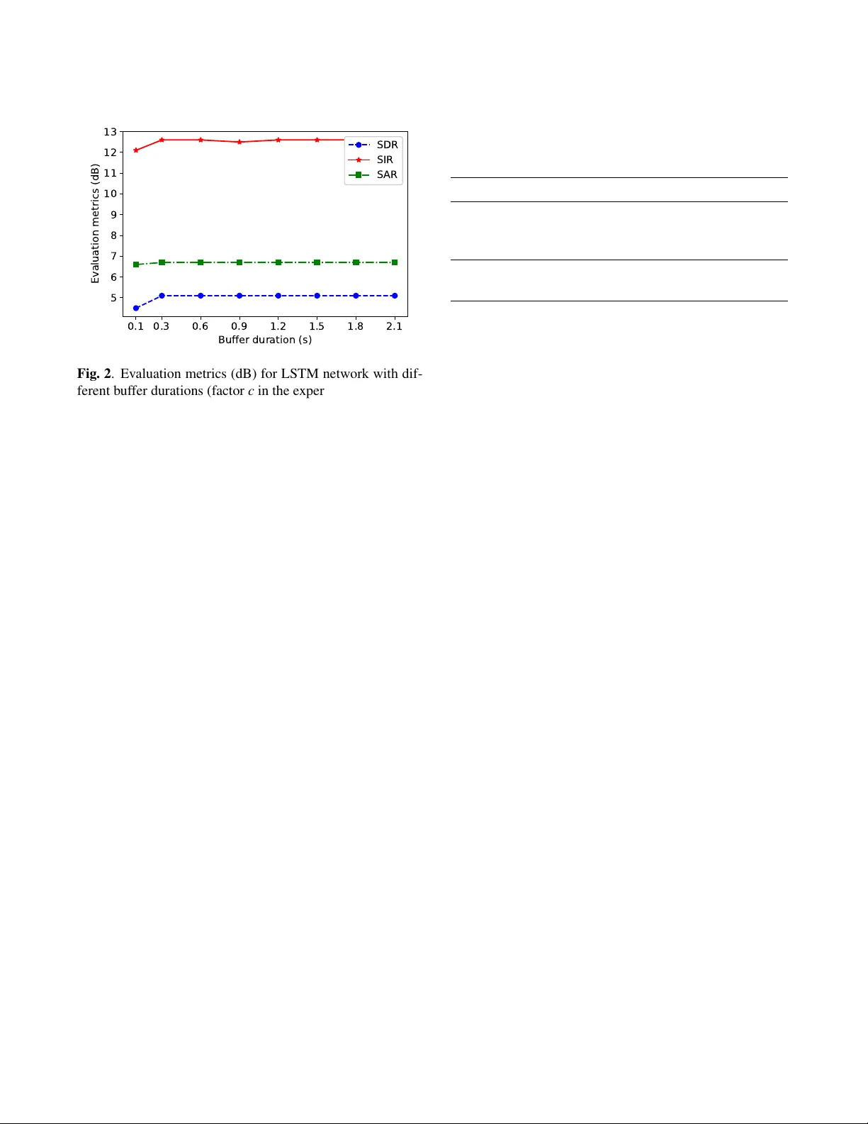
LO W -LA TENCY DEEP CLUSTERING FOR SPEECH SEP ARA TION Shanshan W ang , Gaurav Naithani, T uomas V irtanen Laboratory of Signal Processing, T ampere Uni versity of T echnology , T ampere, Finland Email: { shanshan.2.wang, gaura v .naithani, tuomas.virtanen } @tut.fi ABSTRA CT This paper proposes a low algorithmic latency adaptation of the deep clustering approach to speaker-independent speech separation. It consists of three parts: a) the usage of long- short-term-memory (LSTM) networks instead of their bidi- rectional v ariant used in the original work, b) using a short synthesis windo w (here 8 ms) required for lo w-latency oper - ation, and, c) using a b uffer in the be ginning of audio mixture to estimate cluster centres corresponding to constituent speak- ers which are then utilized to separate speakers within the rest of the signal. The buf fer duration would serve as an initial- ization phase after which the system is capable of operating with 8 ms algorithmic latency . W e e v aluate our proposed approach on two-speaker mixtures from W all Street Journal (WSJ0) corpus. W e observ e that the use of LSTM yields around one dB lo wer SDR as compared to the baseline bidi- rectional LSTM in terms of source to distortion ratio (SDR). Moreov er , using an 8 ms synthesis windo w instead of 32 ms degrades the separation performance by around 2.1 dB as compared to the baseline. Finally , we also report separation performance with different buf fer durations noting that sepa- ration can be achie ved e ven for buf fer duration as low as 300 ms. Index T erms — Monaural speech separation, Low la- tency , Deep clustering. 1. INTR ODUCTION Single channel speech separation is the problem of recover - ing the constituent speech signals from an acoustic mixture signal when information from only a single microphone is av ailable [1]. In recent years, data-dri ven methods relying on deep neural networks (DNN) [2, 3] have yielded dramatic im- prov ements in performance in comparison to the previously used methods, e.g., model-based approaches [4]) and matrix factorization [5, 6]. In particular, speaker-independent speech separation has been addressed by approaches lik e deep clus- tering [7, 8], permutation in v ariant training [9], and more recently deep attractor networks [10] which is the current state-of-the-art. Improvements to the original deep clustering The authors wish to thank CSC-IT Centre of Science Ltd., Finland, for providing computational resources used in experiments reported in this paper . framew ork [7] ha ve been proposed in terms of, e.g., better objectiv e functions [11]; and, improv ed regularization and curriculum training [8]. These studies have considered of- fline separation scenario where the signal to be separated is av ailable at once. Low-latenc y processing is important when these DNN- based methods are applied to applications lik e hearing aids [12] and cochlear implants [13], In particular , for hearing aids, the latency requirements are quite restrictive as the sound is perceived by the listener via hearing aid as well as the direct path. Sev eral studies have documented the sub- jectiv e disturbance experienced by the listeners (e.g., [14]). Notably , Agne w et al . [15] found the delays abo ve 10 ms to be objectionable while delays as low as 3 to 5 ms to be noticeable by hearing-impaired listeners. For the above applications, the of fline DNN-based meth- ods run into two main problems. Firstly , we do not have access to the future temporal information hence DNN models like bidirectional long-short-term-memory netw orks (BLSTM), as used in [3, 16, 7, 8], cannot be used. Secondly , for short- time Fourier transform (STFT) based systems, the algorithmic latency is at least equal to the frame length of synthesis win- dow used for signal reconstruction. This limits us from using window sizes used in con ventional speech processing ( e.g., 20 -40 ms [17]). Speech separation methods with algorithmic latencies belo w 10 ms ha ve been reported, e.g., using non- negati ve matrix factorization [18], and DNNs [19, 20, 21]. In this paper , we in vestigate a lo w-latency adaption of the deep clustering frame work first introduced in [7]. The origi- nal frame work in volves using a BLSTM network to estimate high-dimensional embeddings for each time-frequency bin in the mixture STFT which is then partitioned into clusters cor - responding to the constituent speakers. Our focus in this w ork is three-fold: a) in vestigation of separation performance with LSTM instead of BLSTM to allow online processing, b) in- vestigation of separation performance for short synthesis win- dow (8 ms in this work) instead of longer 32 ms used in orig- inal work, and c) in vestigation of using a certain duration in the beginning of acoustic mixture to estimate the cluster cen- tres corresponding to the constituent sources. W e refer to this time duration as the b uffer . The estimation of cluster centres here thus serves as an initialization phase and the method is capable of doing online separation after the buf fer duration. W e e valuate separately the effect of the above three mod- ifications. W e observ e one dB lower SDR while using an LSTM instead of the BLSTM network as w as used in the original work [7]. The separation performance degrades by around 2.1 dB while shortening the window length from 32 ms to 8 ms as compared to the baseline. Moreover , we show that it is possible to estimate reasonably well cluster centres using just the beginning of the signal yielding good separation for the rest of the signal. The paper is structured as follo ws: Section 2 describes the baseline deep clustering approach proposed in [7]. Section 3 describes its lo w-latency adaptation. Section 4 describes the ev aluation procedure, experimental set up, and obtained results. Finally , Section 5 concludes the paper . 2. DEEP CLUSTERING FOR SPEAKER SEP ARA TION In this section, we summarize the deep clustering method pro- posed in [7, 8]. Deep clustering can be thought of as a com- bination of supervised learning and unsupervised learning. Unlike the traditional DNN-based speech separation methods that predict a time-frequency mask or separate speech spec- trum for the mixture input in a supervised manner [2, 3], it generates an embedding vector for each time-frequency bin and then uses the unsupervised learning approach such as k- means to cluster the embedding vectors in order to get the time-frequency masks. Giv en a mixture audio signal in the time domain x ( n ) , firstly , features are e xtracted by calculating its log magnitude short-time Fourier transform (STFT). The features are then inputted to a neural network that will output an embedding vector for each of the time-frequency points. In the original deep clustering frame work, BLSTM network was used [7], and therefore we choose it as the baseline here. The output of the neural networks is an embedding matrix V ∈ R T F × D , where T denotes the number of frames, F the number of fre- quency bins, and D the embedding dimension. Finally , k- means clustering is employed to partition the embedding vec- tors into clusters corresponding to different constituent speak- ers. Binary time-frequency masks for each speaker is then obtained using these cluster assignments by assigning 1 to all the time-frequency bins within the cluster of the speaker , and 0 to the rest of the bins. The neural network is trained to minimize the dif ference between the estimated affinity matrix VV T deriv ed from the embeddings V predicted by the neural network and the target affinity matrix YY T , where Y ∈ R T F × C is the ideal binary mask. C indicates the number of speakers in the mixture. The training loss function L is computed as, L =    VV T − YY T    F =   V T V   2 F − 2   V T Y   2 F +   Y T Y   2 F , (1) Mixed speech Binary mask Separated speech mask LSTM K-means iSTFT Embeddings STFT Buffer duration (e.g. the first1.5s) Embeddings of the rest of signal Fig. 1 . The block diagram of the proposed low-latenc y deep clustering method. where F denotes the Frobenius norm of the matrix. In or- der to remove the contribution of noisy/silent regions in the network training, a voice activ e detection (V AD) threshold is employed. Only the embeddings corresponding to time- frequency bins with magnitude greater than the V AD thresh- old (-40 dB below the maximum amplitude as in [7]) con- tribute to the abo ve loss calculation. It should be noted that at the test stage the k-means algo- rithm is employed to cluster the embeddings using the entire test signal, thus making the method unsuitable for low-latenc y processing. In the test stage, the estimated binary masks are applied to the complex spectrogram of the mixture hence mix- ture phase is utilized. In verse STFT and overlap-add process- ing is applied to obtain separated signals in the time domain. 3. LO W -LA TENCY DEEP CLUSTERING In order to make the deep clustering based separation oper- ate with low latency , there are three parts that need to be adapted: a) The topology of the neural network is changed from BLSTM as w as used in [7] to LSTM in order to produce embedding vectors in an online manner for each frame as the y are inputted to the netw ork; b) In the baseline method [7], 32 ms synthesis windo w length is used. The resulting latenc y may be prohibiti ve for certain applications, e.g., hearing aids [15] as w as e xplained in the introduction. Hence we shorten the windo w length to 8 ms; and; c) Instead of using the whole signal, we propose using only a certain length in the begin- ning of the mixture, which we refer as the buf fer , to get the cluster centres. These cluster centres can be then used to es- timate the masks for the rest of the mixture. Please note that since the first few seconds of the signal are used to estimate the cluster centres, the method is not able to separate sources during this initialization stage. Ho wever , after the b uf fer , the rest of the signal will be processed in an online manner . The process of the low-latenc y version of deep clustering method is depicted in Fig. 1 with a buf fer duration of 1.5 s. 4. EV ALU A TION 4.1. Acoustic material The e v aluation is done using synthetic two-speaker mixtures generated from W all Street Journal (WSJ0) corpus. The du- ration of mixtures is on av erage around 6 s. The training data set consists of 20,000 two-speaker mixtures created by ran- domly selecting utterances from 101 different speakers from WSJ0 si tr s that amounts to around 30 hours of training ma- terial. Similarly , for the validation data set, we create 5000 two-speaker mixtures that last for around 8 hours having the same speakers as in training data set. The test data is gen- erated from WSJ0 si dt 05 and si et 05 and consists of 3000 mixtures and lasts around 5 hours ha ving 18 dif ferent speak- ers. The test data has different speakers from training data and validation data for the purpose of ev aluating the separa- tion performance in open conditions as described in [7]. W e downsample the speech samples from 16 kHz to 8 kHz for reducing the computational requirements and to make the ev aluation setup similar to [7]. As the proposed approach (factor c ) relies on both the speakers being activ e during the buf fer duration, for a fair in vestigation of the ef fect of buf fer duration and comparison of offline deep clustering to its on- line counterpart, the same data should be used for e v aluation. Hence in the test set for ( c ) we firstly remo ve the silence from the beginning of both speech signals and sum them to form the mixture thus ensuring that both speakers are active during the buffer duration ( ≥ 100 ms in this w ork, i.e., all mixtures hav e both speakers activ e within at least 100 ms in the begin- ning). The longer speech signal is trimmed to the length of the shorter utterance before adding to form the mixture. It should also be noted that such test mixtures have a larger de gree of ov erlapped speech and are thus harder to separate. 4.2. Metrics W e use BSS-EV AL toolbox [22] for ev aluating the system performance. It consists of three metrics: signal-to-distortion- ratio (SDR), signal-to-interference-ratio (SIR), and signal-to- artifacts-ratio (SAR). The a verage SDR of test mixtures with- out any separation is 0.1 dB. 4.3. Experiment setup In order to analyze the effect of the following different fac- tors, namely , a) BLSTM vs LSTM networks, b) 32 ms vs 8 ms window length, and, c) different buf fer duration for lo w- latency process, we conduct separate experiment for each of these. The baseline framework is taken to be the one used in [7]. It consists of a BLSTM netw ork with four layers and 600 units in each layer follo wed by a time-distributed dense layer . The number of units in the time distributed dense layer is the prod- uct of the number of embedding dimensions and the number of ef fectiv e FFT points. Hyperbolic tangent (tanh) is used as the activ ation function in this layer . After the dense layer , L2 normalization is used to bound the embedding vectors to unit norm. The same parameters hav e been used for the LSTM network in order to analyze the effect of factor a) . T o compare the effect of dif ferent windo w length, the same LSTM net- work and a shorter windo w length of 8 ms for STFT feature extraction are used. For a fair comparison with the baseline, the network must be trained with the sequences ha ving the same time conte xt. The baseline BLSTM was trained on 100 frame sequences (800 ms). Here we reduce the hop length to 4 ms hence the sequence length is increased to 200 (800 ms). W e first train the network for 100 frame sequences and then after conv ergence continue training with 200 frame se- quences, known as curriculum learning used in [8] and first introduced in [23]. The idea is to pre-train a network on an easier task first improv es learning and generalization. Finally , c) is studied by v arying the buf fer duration using the network with the same LSTM network (four layers and 600 units in each layer) with 8 ms window length. The same FFT size (256) is used for both of fline (32 and 8 ms frame length) and online deep clustering (8 ms frame length) frame works, i.e., T able 1 . Feature and system parameters for offline and online deep clustering experiments. offline DC low-latenc y DC W indow length 32 ms 8 ms Hop length 8 ms 4 ms Sequence length 100 200 Network BLSTM LSTM W indow Hanning Sampling frequency 8 kHz FFT size 256 Number of layers 4 Number of LSTM units 600 Embedding dimension 40 0 . 1 0 . 3 0 . 6 0 . 9 1 . 2 1 . 5 1 . 8 2 . 1 Bu f f e r d u r a t i o n ( s) 5 6 7 8 9 1 0 1 1 1 2 1 3 E v a l u a t i o n m e t r i c s ( d B) S DR S I R S A R Fig. 2 . Ev aluation metrics (dB) for LSTM network with dif- ferent buf fer durations (factor c in the experimental set up.) zero padding is used wherev er required. During the training process, the ’Adam’ optimizer is uti- lized [24]. The Keras [25] and T ensorflo w [26] libraries are used for network training, and Librosa library [27] is used for feature e xtraction and signal reconstruction in this paper . In order to reduce overfitting, early stopping method is used [28] by monitoring the loss on validation data and stopping the training when no decrease in it is observed for 30 epochs. The embedding dimension is set to 40 and the V AD thres hold is 40 dB, similar to the original study [7]. The detailed de- scription of the parameters for the network can be found from T able 1. It should be noted that Fig. 1 depicts the real world use case where a buf fer duration in the beginning of an utterance is used for estimating clusters and the separation starts after that. This howe ver makes acoustic material used for ev alu- ation dependent upon the b uffer duration if the same utter- ance is used for both cluster estimation and e valuation. T o deal with this mismatch, for each test utterance, we randomly select another utterance (cluster utterance) belonging to the same speaker pair and use it to estimate clusters. Different buf fer lengths can thus be sampled from the beginning of this cluster utterance for the same test utterance in order to study the effect of factor c . Moreover , the V AD threshold is used during cluster estimation to exclude the ef fect of noisy time- frequency bins. 4.4. Results and discussion W e calculate the mean of ev aluation metrics, SDR, SIR, and SAR ov er all the test mixtures. All the test mixtures are formed such that both constituent speech signals are activ e within the lowest buf fer duration used in experiments (100 ms here). Hence they hav e a higher overlap between the con- stituent speech. As described in the previous section, we T able 2 . Evaluation metrics (dB) of dif ferent variants of the offline method and the online method with 1.5s buf fer . Here online refers to factor c in the experimental setup W indow length SDR SIR SAR BLSTM 32 ms 7.9 15.6 9.2 LSTM 32 ms 6.9 14.5 8.4 LSTM 8 ms 5.8 13.6 7.2 Online LSTM 8 ms 5.1 12.6 6.7 (1.5s buf fer) adopt the strategy of estimating clusters on dif ferent utter- ances than test utterances. Hence the same dataset can be used for ev aluation for both offline and online deep cluster- ing methods. The results with baseline offline case is shown in T able 2. Similarly , the ev aluation metrics corresponding to the LSTM network with 32 and 8 ms window lengths is shown as well. The online LSTM in T able 2 refers to low- latency LSTM with 8 ms window length and 1.5 s buf fer time. It can be observed that the separation performance is one dB lower in terms of SDR while replacing BLSTM to LSTM while k eeping the same window length. Moreo ver , by decreasing the window length to 8 ms, SDR degrades by about 2.1 dB as compared to the baseline. The effect of varying buf fer duration on performance met- rics is shown in Fig. 2. T wo interesting observations can be made from it: firstly , ev en with a short buf fer duration, e.g., 100 ms, relatively reasonable separation performance can still be achiev ed (4.5 dB); and secondly after a certain buffer length more information does not lead to a drastic improve- ment in separation performance. This means a small buf fer duration, ev en as low as 300 ms, can yield good separation provided both the constituent speakers are acti ve during it. 5. CONCLUSION The paper proposes a lo w-latency adaptation of deep clus- tering based speech separation. In particular, a buffer signal duration in the beginning of audio mixture is used for esti- mating cluster centres corresponding to the speakers present in the mixture. This duration serv es as an ’initialization’ pe- riod after which the rest of the speech mixture is processed in online manner . Moreover , separation performance of the method using an LSTM network and a short synthesis win- dow length of 8 ms, as required by real-time operation, has been studied. A degradation in SDR of about one dB is ob- served for the former and 2.1 dB for the latter as compared to the baseline. Finally , we inv estigate how the buf fer duration affects the separation result and observ e that e ven very short buf fer duration, e.g. 300 ms, is suf ficient to estimate clusters for reasonable separation. 6. REFERENCES [1] E. V incent, T . V irtanen, and S. Gannot, Audio sour ce separa- tion and speech enhancement . John W iley & Sons, 2018. [2] P . Huang, M. Kim, M. Hasega wa-Johnson, and P . Smaragdis, “Deep learning for monaural speech separation, ” in Proc. IEEE International Confer ence on Acoustics, Speech and Signal Pr o- cessing , 2014, pp. 1562–1566. [3] H. Erdogan, J. R. Hershey , S. W atanabe, and J. Le Roux, “Phase-sensitiv e and recognition-boosted speech separation using deep recurrent neural networks, ” in Proc. IEEE Interna- tional Conference on Acoustics, Speech and Signal Pr ocessing (ICASSP) , 2015, pp. 708–712. [4] S. T . Roweis, “One microphone source separation, ” in Pr oc. Advances in Neural Information Pr ocessing Systems (NIPS) , 2001, pp. 793–799. [5] T . V irtanen, “Monaural sound source separation by nonnega- tiv e matrix factorization with temporal continuity and sparse- ness criteria, ” IEEE T ransactions on A udio, Speech, and Lan- guage Pr ocessing , vol. 15, no. 3, pp. 1066–1074, 2007. [6] M. N. Schmidt and R. K. Olsson, “Single-channel speech separation using sparse non-ne gati ve matrix factorization, ” in Pr oc. International Conference on Spoken Language Pr ocess- ing , 2006. [7] J. R. Hershey , Z. Chen, J. Le Roux, and S. W atanabe, “Deep clustering: Discriminativ e embeddings for segmentation and separation, ” in Pr oc. IEEE International Conference on Acous- tics, Speech and Signal Pr ocessing (ICASSP) , 2016, pp. 31–35. [8] Y . Isik, J. L. Roux, Z. Chen, S. W atanabe, and J. R. Hershey , “Single-channel multi-speaker separation using deep clustering, ” in Pr oc. Interspeech , 2016, pp. 545–549. [Online]. A v ailable: http://dx.doi.or g/10.21437/Interspeech.2016- 1176 [9] D. Y u, M. Kolbæk, Z.-H. T an, and J. Jensen, “Permutation in- variant training of deep models for speak er-independent multi- talker speech separation, ” in Pr oc. IEEE International Confer- ence on Acoustics, Speech and Signal Pr ocessing (ICASSP) , 2017, pp. 241–245. [10] Z. Chen, Y . Luo, and N. Mesgarani, “Deep attractor network for single-microphone speak er separation, ” in Pr oc. IEEE In- ternational Confer ence on Acoustics, Speech and Signal Pr o- cessing (ICASSP) , 2017, pp. 246–250. [11] Z.-Q. W ang, J. Le Roux, and J. R. Hershey , “ Alternativ e ob- jectiv e functions for deep clustering, ” in Pr oc. IEEE Interna- tional Conference on Acoustics, Speech and Signal Pr ocessing (ICASSP) , 2018, pp. 686–690. [12] L. Bramsløw , “Preferred signal path delay and high-pass cut-off in open fittings, ” International Journal of Audiology , vol. 49, no. 9, pp. 634–644, 2010. [13] J. Hidalgo, “Low latency audio source separation for speech enhancement in cochlear implants, ” Master’ s thesis, Universi- tat Pompeu Fabra, 2012. [14] M. A. Stone, B. C. Moore, K. Meisenbacher , and R. P . Derleth, “T olerable hearing aid delays. V. estimation of limits for open canal fittings, ” Ear and Hearing , v ol. 29, no. 4, pp. 601–617, 2008. [15] J. Agnew and J. M. Thornton, “Just noticeable and objection- able group delays in digital hearing aids, ” J ournal of the Amer- ican Academy of Audiology , vol. 11, no. 6, pp. 330–336, 2000. [16] Z. Chen, S. W atanabe, H. Erdogan, and J. R. Hershe y , “Speech enhancement and recognition using multi-task learning of long short-term memory recurrent neural networks, ” in Pr oc. Inter- speech , 2015. [17] K. K. Paliwal, J. L yons, and K. W ojcicki, “Preference for 20-40 ms window duration in speech analysis, ” in Pr oc. International Confer ence on Signal Pr ocessing and Communication Systems (ICSPCS) , 2011, pp. 1 – 4. [18] T . Barker , T . V irtanen, and N. H. Pontoppidan, “Low-latency sound-source-separation using non-negati ve matrix factorisa- tion with coupled analysis and synthesis dictionaries, ” in Pr oc. IEEE International Conference on Acoustics, Speech and Sig- nal Pr ocessing (ICASSP) , 2015, pp. 241–245. [19] G. Naithani, T . Barker , G. Parascandolo, L. Bramsløw , N. H. Pontoppidan, and T . V irtanen, “Low latenc y sound source separation using conv olutional recurrent neural networks, ” in Pr oc. IEEE W orkshop on Applications of Signal Processing to Audio and Acoustics (W ASP AA) , 2017, pp. 71–75. [20] G. Naithani, G. Parascandolo, T . Barker, N. H. Pontoppidan, and T . V irtanen, “Low-latenc y sound source separation us- ing deep neural networks, ” in Pr oc. IEEE Global Confer ence on Signal and Information Processing (GlobalSIP) , 2016, pp. 272–276. [21] Y . Luo and N. Mesgarani, “T asNet: time-domain audio sepa- ration network for real-time single-channel speech separation, ” in Proc. IEEE International Confer ence on Acoustics, Speech and Signal Pr ocessing (ICASSP) , 2018, pp. 696–700. [22] E. V incent, R. Gribonv al, and C. F ´ evotte, “Performance mea- surement in blind audio source separation, ” IEEE T ransactions on Audio, Speec h, and Languag e Pr ocessing , v ol. 14, no. 4, pp. 1462–1469, 2006. [23] Y . Bengio, J. Louradour , R. Collobert, and J. W eston, “Curricu- lum learning, ” in Pr oc. International Conference on Machine Learning (ICML) , 2009, pp. 41–48. [24] D. Kingma and J. Ba, “ Adam: A method for stochastic opti- mization, ” in Pr oc. International Conference on Learning Rep- r esentations , 2014. [25] F . Chollet et al. , “K eras, ” 2015. [Online]. A vailable: https://github .com/fchollet/keras [26] M. Abadi et al. , “T ensorflow: A system for large-scale machine learning, ” in Pr oc. USENIX Symposium on Operating Systems Design and Implementation (OSDI) , 2016, pp. 265–283. [27] B. McFee et al. , “librosa 0.5.0, ” Feb . 2017. [Online]. A v ailable: https://doi.or g/10.5281/zenodo.293021 [28] R. Caruana, S. Lawrence, and L. Giles, “Ov erfitting in neu- ral nets: Backpropagation, conjugate gradient, and early stop- ping, ” in Proc. Advances in Neural Information Processing Systems (NIPS) , vol. 13, 2001, p. 402.