Randomly weighted CNNs for (music) audio classification

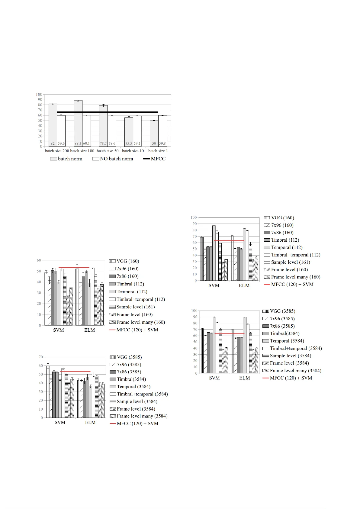
RANDOML Y WEIGHTED CNNs FOR (MUSIC) A UDIO CLASSIFICA TION Jordi P ons Music T echnology Group Uni versitat Pomepeu Fabra, Barcelona Xa vier Serra Music T echnology Group Uni versitat Pomepeu Fabra, Barcelona ABSTRA CT The computer vision literature shows that randomly weighted neural networks perform reasonably as feature extractors. Follo wing this idea, we study how non-trained (randomly weighted) con volutional neural networks per- form as feature extractors for (music) audio classification tasks. W e use features extracted from the embeddings of deep architectures as input to a classifier – with the goal to compare classification accuracies when using different ran- domly weighted architectures. By follo wing this method- ology , we run a comprehensive ev aluation of the current deep architectures for audio classification, and provide ev- idence that the architectures alone are an important piece for resolving (music) audio problems using deep neural networks. 1. MO TIV A TION – FR OM PREVIOUS WORKS Some intriguing properties of deep neural networks are pe- riodically sho wing up in the scientific literature. Examples of those are: (i) perceptually non-relev ant signal pertur- bations that dramatically affect the predictions of an im- age classifier [12, 49]; (ii) although there is no guaran- tee of con verging to a global minima that might general- ize, image classification models perform well with unseen data [14, 25]; or (iii) non-trained deep neural networks are able to perform reasonably well as image feature extrac- tors [41, 43, 51]. In this work, we exploit one of the abov e listed properties (iii) to ev aluate how discriminativ e deep audio architectures are before training. Previous works already explored the idea of empirically studying the qualities of non-trained (randomly weighted) networks, b ut mainly in the computer vision field: · Saxe et al. [43] studied how discriminativ e are the ar- chitectures themselv es by e valuating the classification per- formance of SVMs fed with features extracted from non- trained (random) CNNs. 1 They showed that a surprising fraction of the performance in deep image classifiers can be attributed to the architecture alone. Therefore, the key to good performance lies not only on improving the learn- ing algorithms but also in searching for the most suitable architectures. Further , the y sho wed that the (classification) 1 CNNs stands for Con volutional Neural Networks. c  Jordi Pons, Xavier Serra. Licensed under a Creativ e Commons Attrib ution 4.0 International License (CC BY 4.0). Attribu- tion: Jordi Pons, Xavier Serra. “Randomly weighted CNNs for (music) audio classification” performance deliv ered by random CNN features is corre- lated with the results of their end-to-end trained counter- parts – this result means, in practice, that one can bypass the time-consuming process of learning for ev aluating a giv en architecture. W e build on top of this result to ev alu- ate current CNN architectures for audio classification. · Rosenfeld and Tsotsos [41] fixed most of the model’ s weights to be random, and only allowed a small portion of them to be learned. By following this methodology , they showed a small decrease in image classification per- formance when these models were compared to their fully trained counterparts. Further, the performance of their non fully-trained models can be summarized as follows: DenseNet [17]  ResNet [15] > VGG [48]  AlexNet [25] What matches previous works reporting how these (fully trained) models perform [15, 17, 48], confirming the per- formance correlation between randomly weighted models and their trained counterparts found by Saxe et al. [43] · Adebayo et al. [1] empirically assessed the local ex- planations of deep image classifiers to find that randomly weighted models produce explanations similar to those produced by models with learned weights. They conclude that the architectures introduce a strong prior which af fects the learned (and not learned) representations. · Ulyanov et al. [51] also showed that the structure of a network (the non-trained architecture) is sufficient to cap- ture useful features for the tasks of image denoising, super- resolution and inpainting. They think of any designed ar- chitecture as a hand-crafted model where prior informa- tion is embedded in the structure of the network itself. This way of thinking resonates with the rationale behind the family of audio models designed considering domain knowledge (see section 2) – what denotes that in both audio and image fields it exists the interest of bringing together the end-to-end learning literature and previous research. Few related works exist in the audio field – and ev- ery randomly weighted neural network we found in the audio literature was a mere baseline [2, 7, 24]. Inspired by previous computer vision works, we study which au- dio architectures work the best via ev aluating how non- trained CNNs perform as feature extractors. T o this end, we use the CNNs’ embeddings to construct feature vec- tors for a classifier – with the goal to compare classifica- tion performances when different randomly weighted ar- chitectures are used to extract features. T o the best of our knowledge, this is the first comprehensiv e ev aluation of randomly weighted CNNs for (music) audio classification. Figure 1 . CNN front-ends for audio classification tasks – with examples of possible configurations for e very paradigm. Extreme learning machines (ELMs) [18, 32, 47] and echo state networks (ESNs) [19] are also closely related to our work. In short, ELMs are classification/regression models 2 that are based on a single-layer feed-forward neu- ral network with random weights. They work as follows: first, ELMs randomly project the input into a latent space; and then, learn ho w to predict the output via a least-square fit. More formally , we aim to predict: ˆ Y = W 2 σ ( W 1 X ) , where W 1 is the (randomly weighted) matrix of input-to- hidden-layer weights, σ is the non-linearity , W 2 is the ma- trix of hidden-to-output-layer weights, and X represents the input. The training algorithm is as follows: 1) set W 1 with random v alues; 2) estimate W 2 via a least-squares fit: W 2 = σ ( W 1 X ) + Y where + denotes the Moore-Penrose in verse. Since no iter- ativ e process is required for learning the weights, training is faster than stochastic gradient descent [18]. Provided that we process audio signals with randomly weighted CNNs, ELM-based classifiers are a natural choice for our study – so that all the pipeline (except the last layer) is based on random projections that are only constrained by the structure of the neural network. Although ELMs are not widely used by the audio community , they hav e been used for speech emotion recognition [13, 21], or for music audio classification [23, 29, 44]. ESNs differ from ELMs in that their random projections use recurrent connections. Giv en that the audio models we aim to study are not recur - rent, we lea ve for future work using ESNs – see [16, 45] for audio applications of ESNs. 2. ARCHITECTURES In this work we evaluate the most used deep learning archi- tectures for (music) audio classification. In order to facil- itate the discussion around these architectures, we divide 2 Support V ector Machines are also classification/re gression models. the deep learning pipeline into two parts: front-end and back-end, see Figure 2. The front-end is the part that inter- acts with the input signal in order to map it into a latent- space, and the back-end predicts the output giv en the rep- resentation obtained by the front-end. Note that one can in- terpret the front-end as a “feature extractor” and the back- end as a “classifier”. Giv en that we compare how several non-trained (random) CNNs perform as feature extractors, and we will use out-of-the-box classifiers to predict the classes: this literature revie w focuses in introducing the main deep learning front-ends for audio classification. Figure 2 . The deep learning pipeline. F ront-ends — These are generally conformed by CNNs [6, 9, 38, 39, 53], since these can encode ef ficient represen- tations by sharing weights 3 along the signal. Figure 1 de- picts six different CNN front-end paradigms, which can be divided into two groups depending on the used input sig- nal: wa veforms [9, 27, 53] or spectrograms [6, 38, 39]. Fur- ther , the design of the filters can be either based on domain knowledge or not. For example, one lev erages domain knowledge when the frame-level single-shape 4 front-end for wav eforms is designed so that the length of the filter is set to be the same as the window length in a STFT [9]. Or for a spectrogram front-end, it is used vertical filters to learn spectral representations [26] or horizontal filters to learn longer temporal cues [46]. Generally , a single fil- ter shape is used in the first CNN layer [6, 9, 26, 46], but some recent work reported performance gains when using sev eral filter shapes in the first layer [5, 34, 36, 38, 39, 53]. Using many filters promotes a more rich feature extrac- tion in the first layer , and facilitates leveraging domain knowledge for designing the filters’ shape. For exam- 3 Which constitute the (ev entually learnt) feature representations. 4 Italicized names correspond to the front-end types in Figure 1. ple: a frame-level many-shapes front-end for wav eforms can be motiv ated from a multi-resolution time-frequency transform 5 perspectiv e – with window sizes varying in- versely with frequenc y [53]; or since it is known that some patterns in spectrograms are occurring at different time- frequency scales, one can intuitively incorporate many ver- tical and/or horizontal filters to efficiently capture those in a spectrogram front-end [34, 36, 38, 39]. As seen, using domain knowledge when designing the models allows to naturally connect the deep learning literature with previ- ous relevant signal processing work. On the other hand, when domain knowledge is not used, it is common to em- ploy a deep stack of small filters, e.g.: 3 × 1 in the sample- level front-end used for wa veforms [27, 40, 52], or 3 × 3 in the small-rectangular filters front-end used for spectro- grams [6]. These VGG-like 6 models make minimal as- sumptions o ver the local stationarities of the signal, so that any structure can be learnt via hierarchically combining small-context representations. 3. METHOD Our goal is to study which CNN front-ends work best via ev aluating how non-trained models perform as feature ex- tractors. Our e v aluation is based on the traditional pipeline of featur es extraction + classifier . W e use the embed- dings of non-trained (random) CNNs as features: for e very audio clip, we compute the average of each feature map (in ev ery layer) and concatenate these values to construct a feature vector [7]. The baseline feature vector is con- structed from 20 MFCCs, their ∆ s and ∆∆ s. W e compute their mean and standard deviation through time, and the resulting feature vector is of size 120. W e set the widely used MFCCs + SVM setup as baseline. T o allo w a fair comparison with the baseline, CNN models hav e ≈ 120 feature maps – so that the resulting feature vectors hav e a similar size as the MFCCs vector . Further , we ev aluate an alternativ e configuration with more feature maps ( ≈ 3500) to show the potential of this approach. Model’ s descrip- tion omit the number of filters per layer for simplicity – full implementation details are accessible online. 8 3.1 Featur es: randomly weighted CNNs Except for the VGG model that uses ELUs as non- linearities [6, 8], the rest use ReLUs [10] – and we do not use batch normalization, see discussion in section 3.4. W e use wa veforms and spectrograms as input to our CNNs: W av eform inputs — are of ≈ 29sec (350,000 samples at 12kHz) and the following architectures are under study: · Sample-level: is based on a stack of 7 blocks that are composed by a 1D-CNN layer (filter length: 3, stride: 1) and a max-pool layer (size: 3, stride: 3) – with the excep- tion of the input block which has no max-pooling and its 1D-CNN layer has a stride of 3 [27]. A verages to construct the feature vector are computed after every pooling layer , except for the first layer that are computed after the CNN. 5 The Constant-Q T ransform [3] is an example of such transform. 6 VGG: a computer vision model based on a deep stack of 3 × 3 filters. · F rame-level many-shapes: consists of a 1D-CNN layer with five filter lengths: 512, 256, 128, 64, 32 [53]. Every filter’ s stride is of 32 and we use same padding – to easily concatenate feature maps of the same size. Note that out of this single 1D-CNN layer , five feature maps (result- ing of the different filter length conv olutions) are concate- nated. For that reason, e very feature map needs to ha ve the same (temporal) size. Since this model is single-layered and it might be in clear disadvantage when compared to the sample-level CNN, we increase its depth via adding three more 1D-CNN layers (length: 7, stride: 1) – where the last two layers hav e residual connections, and the penultimate layer’ s feature map is down-sampled by two (MP x2), see Figure 3. A verages to construct the feature vector are cal- culated for each feature map after ev ery 1D-CNN layer . · F rame-level: consists of a 1D-CNN layer with a filter of length 512 [9]. Stride is set to be 32 to allo w a fair com- parison with the frame-le vel many-shapes architecture. As in frame-level many-shapes , we increase the depth of the model via adding three more 1D-CNN layers – as in Fig- ure 3. A verages to construct the feature vector are calcu- lated for each feature map after ev ery 1D-CNN layer . Figure 3 . Additional layers for the frame-level & frame- level many-shapes architectures, similar as in [9, 37] – where MP stands for max pooling. Spectrogram inputs — are set to be log-mel spectrograms (spectrograms size: 1376 × 96 7 , being ≈ 29sec of signal). Differently from waveform models, spectrogram architec- tures use no additional layers to deepen single-layered CNNs because these already deliv er a reasonable classi- fication performance. Unless we state the contrary , every CNN layer used for processing spectrograms is set to ha ve stride 1. As for the frame-level many-shapes model, we use same padding when ma ny filter shapes are used in the same layer . The following spectrogram models are studied: · 7 × 96 : consists of a single 1D-CNN layer with filters of length 7 that con volve through the time axis [9]. As a result: CNN filters are vertical and of shape 7 × 96. There- fore, these filters can encode spectral (timbral) representa- tions. A verages to construct the feature vector are calcu- lated for each feature map after the 1D-CNN layer . · 7 × 86 : consists of a single 2D-CNN layer with verti- cal filters of shape 7 × 86 [36, 39]. Since its vertical shape is smaller than the input (86 < 96), filters can also con volv e through the frequency axis – what can be seen as “pitch shifting” the filter . Consequently , 7 × 86 filters can encode pitch-in variant timbral representations [36, 39]. Further , since the resulting activ ations can carry pitch-related in- formation, we max-pool the frequency axis to get pitch- in variant features (max-pool shape: 1 × 11). A verages to construct the feature vector are calculated for each feature map after the max-pool layer . 7 STFT parameters: window size = 512 , hop size=256 , and fs=12kHz . · T imbral : consists of a single 2D-CNN layer with many vertical filters of shapes: 7 × 86, 3 × 86, 1 × 86, 7 × 38, 3 × 38, 1 × 38, see Figure 4 (top) [11, 35, 39]. These filters can also con volv e through the frequency axis and there- fore, these can encode pitch-inv ariant representations. Sev- eral filter shapes are used to ef ficiently capture different timbrically relev ant time-frequency patterns, e.g.: kick- drums (can be captured with 7 × 38 filters representing sub- band information for a short period of time), or string en- semble instruments (can be captured with 1 × 86 filters rep- resenting spectral patterns spread in the frequency axis). Further , since the resulting activ ations can carry pitch- related information, we max-pool the frequenc y axis to get pitch-in variant features (max-pool shapes: 1 × 11 or 1 × 59). A verages to construct the feature vector are calculated for each feature map after the max-pool layer . · T empor al : sev eral 1D-CNN filters (of lengths: 165, 128, 64, 32) operate over an energy env elope obtained via mean-pooling the frequency-axis of the spectrogram, see Figure 4 (bottom). By computing the energy env elope in that way , we are considering high and low frequencies to- gether while minimizing the computations of the model. Observe that this single-layered 1D-CNN is not operating ov er a 2D spectrogram, but over a 1D energy env elope – therefore no vertical con volutions are performed, only 1D (temporal) con volutions are computed. As seen, domain knowledge can also pro vide guidance to (ef fectiv ely) mini- mize the computations of the model. A verages to construct the feature vector are calculated for each feature map after the CNN layer . · T imbral+temporal : combines both timbral and tem- poral CNNs in a single (b ut wide) layer , see Figure 4 [37]. A verages to construct the feature vector are calculated in the same way as for timbral and tempor al architectures. · VGG : is a computer vision model based on a stack of 5 blocks combining 2D-CNN layers (with small rectangular filters of 3 × 3) and max-pooling (of shapes: 4 × 2, 4 × 3, 5 × 2, 4 × 2, 4 × 4, respectively) [6]. A verages to construct the feature vector are computed after every pooling layer . Figure 4 . T imbral+tempor al architecture. MP: max-pool. As seen, studied architectures are representative of the au- dio classification state-of-the-art – introduced in section 2. For further details about the models under study: the code is accessible online 8 , and a graphical conceptualization of the models is av ailable in Figures 1, 3 and 4. 8 https://github.com/jordipons/elmarc 3.2 Classifiers: SVM and ELM W e study ho w sev eral feature vectors (computed consider - ing different CNNs) perform for a giv en set of classifiers: SVMs and ELMs. W e discarded the use of other clas- sifiers since their performance was not competitiv e when compared to those. SVMs and ELMs are hyper-parameter sensitiv e, for that reason we perform a grid search: · SVM hyper-parameters: we consider both linear and rbf kernels. For the rbf kernel, we set γ to: 2 − 3 , 2 − 5 , 2 − 7 , 2 − 9 , 2 − 11 , 2 − 13 , #featur es − 1 ; and for ev ery kernel configuration, we try several C ’ s (penalty parameter): 0.1, 2, 8, 32. W e use scikit-learn’ s SVM implementation [33]. · ELM ’ s main hyper-parameter is the number of hidden units: 100, 250, 500, 1200, 1800, 2500. W e use ReLUs as non-linearity , and we use a public ELM implementation. 9 3.3 Datasets: music and acoustic events · GTZAN fault-filtered version [22, 50]. T raining songs: 443, validation songs: 197, and test songs: 290 – divided in 10 classes. W e use this dataset to study how randomly weighted CNNs perform for music genre classification. · Extended Ballr oom [4, 30] – 4,180 songs divided in 13 classes; 10 stratified folds are randomly generated for cross-validation. W e use this dataset to study how ran- domly weighted CNNs classify rhythm/tempo classes. · Urban Sound 8K [42] – 8732 acoustic events divided in 10 classes; 10 folds are already defined by the dataset au- thors for cross-validation. Since urban sounds are shorter than 4 seconds and our models accepts ≈ 29sec inputs, the signal is repeated to create inputs of the same length. W e use this dataset to study how randomly weighted CNNs perform to classify natural (non-music) sounds. 3.4 Reproducing f ormer results to discuss our method Choi et al. [7] used random CNN features as baseline for their work, and found that (in most cases) these random CNN features perform better than MFCCs. Moti vated by this result, we pursue this idea for studying how differ - ent deep architectures perform when resolving audio prob- lems. T o start, we first reproduce one of their experiments using random CNNs – under the same conditions 10 : the GTZAN dataset is split in 10 stratified folds used for cross- validation 11 , a VGG architecture with batch normaliza- tion is employed, and the classifier is an SVM. W e found that results can vary depending on the batch size if, when computing the feature vectors, layers are normalized with the statistics of current batch (batch normalization). F or example: if audio-features of the same genre are batch- normalized by the same factor , one can create an artifi- cial genr e cue that might affect the results. One can ob- serve this phenomena in Figure 5, where the best results are achieved when all songs of the same genre fill a full batch (batch size of 100). 12 W e also observe that small batch sizes are harming the model’ s performance – see 9 https://github.com/zygmuntz/Python- ELM 10 https://github.com/keunwoochoi/transfer_ learning_music/ (more information is available in issue #2) 11 Our work does not use this split, we use the fault-filtered v ersion. 12 The GTZAN has 10 genres with 100 audios each, one can fill batches of 100 with audios of the same genre via sorting the data by genres. in Figure 5 when batch sizes are set to 1 and 10. And finally , when batch normalization is not used, no mat- ter what batch size we use that the results remain the same – ANO V A test with H 0 being that av erages are equal ( p-value=0.491 ). Since it is not desirable that performance depends on the batch size, and that the feature vector of an audio depends on other audios (that are present in the batch): we decided not to use batch normalization. Figure 5 . Random CNN features behavior when using (or not) batch normalization. Dataset : GTZAN, 10-fold cross- validation. P erformance metric (%) : av erage accuracies (and standard deviations) across 3 runs. Classifier : SVM. 4. RESUL TS Figures show average accuracies across 3 runs for ev ery feature type (listed on the right with the length of the fea- ture vector in parenthesis). W e use a t-test to rev eal which models are performing the best – H 0 : av erages are equal. 4.1 GTZAN: music genre r ecognition Figure 6 . Accuracy (%) results for the GTZAN dataset with random CNN feature vectors of length ≈ 120. Figure 7 . Accuracy (%) results for the GTZAN dataset with random CNN feature vectors of length ≈ 3500. The sample-level wav eform model always performs better than frame-le vel many-shapes (t-test: p-value  0.05). The two best performing spectrogram-based models are: tim- bral+tempor al and VGG – with a remarkable performance of the timbral model alone. The timbral+temporal CNN performs better than VGG when using the ELM ( ≈ 3500) classifier (t-test: p-value=0.017); but in other cases, both models perform equi valently (t-test: p-value > 0.05). Moreov er , the 7x86 model performs better than 7x96 when using SVMs (t-test: p-value < 0.05), but when us- ing ELMs: 7x96 and 7x86 perform equiv alently (t-test: p- value  0.05). The best VGG and timbral+temporal mod- els achieve the following (av erage) accuracies: 59.65% and 56.89%, respectiv ely – both with an SVM ( ≈ 3500) classifier . Both models outperform the MFCCs baseline: 53.44% (t-test: p-value < 0.05), but these random CNNs perform worse than a CNN pre-trained with the Million Song Dataset: 82.1% [28]. Finally , note that although timbral and timbral+temporal models are single-layered, these are able to achieve remarkable performances – sho w- ing that single-layered spectrogram front-ends (attending to musically relev ant contexts) can do a reasonable job without paying the cost of going deep [36, 39]. Thus mean- ing, e.g., that the saved capacity can now be employed by the back-end to learn (some more) representations. 4.2 Extended Ballroom: rhythm/tempo classification Figure 8 . Accuracy (%) results for the Extended Ballroom dataset with random CNN feature vectors of length ≈ 120. Figure 9 . Accuracy (%) results for the Extended Ballroom dataset with random CNN feature vectors of length ≈ 3500 The sample-level wa veform model always performs bet- ter than frame-le vel many-shapes (t-test: p-value  0.05). The two best performing spectrogram-based models are: temporal and timbral+temporal , b ut the tempo- ral model performs better than timbral+temporal in all cases (t-test: p-value  0.05) – denoting that spec- tral cues can be a confounding factor for this dataset. Moreov er , the 7x86 model performs better than 7x96 in all cases (t-test: p-value < 0.05). The best (av er- age) accuracy score is obtained using temporal models and SVMs ( ≈ 3500): 89.82%. Note that the temporal model clearly outperforms the MFCCs baseline: 63.25% (t-test: p-value  0.05) and, interestingly , it performs slightly w orse than a trained CNN: 93.7% [20]. This result confirms that the architectures (alone) introduce a strong prior which can significantly affect the performance of an audio model. Thus meaning that, besides learning, de- signing effecti ve architectures might be key for resolving (music) audio tasks with deep learning. In line with that, note that the temporal architecture is designed consider- ing musical domain knowledge – in this case: how tempo & rhythm are expressed in spectrograms. Hence, its good performance also validates the design strategy of using mu- sically motiv ated architectures as a way to intuitiv ely nav- igate through the network parameters space [36, 38, 39]. 4.3 Urban Sounds 8K: acoustic event detection For these experiments we do not use the temporal model (with 1D-CNNs of length 165, 128, 64, 32). Instead, we study the temporal+time model – where time follows the same design as temporal but with filters of length: 64, 32, 16, 8. This change is moti vated by the fact that temporal cues in (natural) sounds are shorter and less important than temporal cues in music (i.e., rhythm or tempo). Figure 10 . Accuracy (%) results for the Urban Sounds 8k dataset with random CNN feature vectors of length ≈ 120. Figure 11 . Accuracy (%) results for the Urban Sounds 8k dataset with random CNN feature vectors of length ≈ 3500 The sample-level wa veform model always performs bet- ter than frame-le vel many-shapes (t-test: p-value  0.05). The two best performing spectrogram-based models are: VGG and timbral+time – but VGG performs better than timbral+time in all cases (t-test: p-value  0.05). Also, the 7x86 model performs better than 7x96 in all cases (t-test: p-value < 0.075). The best (av erage) accu- racy score is obtained using VGG and SVMs ( ≈ 3500): 70.74% – outperforming the MFCCs baseline: 65.49% (t-test: p-value < 0.05), and performing slightly worse than a trained CNN: 73% 13 [28]. Finally , note that VGG s achiev ed remarkable results when recognizing genres and detecting acoustic e vents – tasks where timbre is an impor- tant cue. As a result: one could argue that VGG s are good at representing spectral features. Hence, these might be of utility for tasks where spectral cues are relev ant. 5. CONCLUSIONS This study builds on top of prior works sho wing that the (classification) performance deliv ered by random CNN features is correlated with the results of their end-to-end trained counterparts [41, 43]. W e use this property to run a comprehensive ev aluation of current deep architectures for (music) audio. Our method is as follows: first, we extract a feature vector from the embeddings of a ran- domly weighted CNN; and then, we input these features to a classifier – which can be an SVM or an ELM. Our goal is to compare the obtained classification accuracies when using different CNN architectures. The results we obtain are far from random , since: (i) randomly weighted CNNs are (in some cases) close to match the accuracies obtained by trained CNNs; and (ii) these are able to out- perform MFCCs. This result denotes that the architectures alone are an important piece of the deep learning solution and therefore, searching for efficient architectures capable to encode the specificities of (music) audio signals might help advancing the state of our field. In line with that, we hav e sho wn that (musical) priors embedded in the structure of the model can facilitate capturing useful (temporal) cues for classifying rhythm/tempo classes. Besides, we show that for wav eform front-ends: sample-level  frame-level many-shapes > frame-level – as noted in the (trained) lit- erature [27, 52, 53]. The differential aspect of the sample- level front-end is that its representational power is con- structed via hierarchically combining small-context repre- sentations, not by exploiting prior knowledge about wav e- forms. Further , we show that for spectrogram front-ends: 7x96 < 7x86 – as shown in prior (trained) works [31, 36]. By allowing the filters to conv olve through the frequency axis, the architecture itself facilitates capturing pitch- in variant timbral representations. Finally: timbral ( +tem- poral/time ) and VGG spectrogram front-ends achiev e re- markable results for tasks where timbre is important – as previously noted in the (trained) literature [39]. Their respectiv e advantages being that: (i) timbral ( +tempo- ral/time ) architectures are single-layered front-ends which explicitly capture acoustically relev ant receptiv e fields – which can be known via exploiting prior knowledge about the task; and (ii) VGG front-ends require no prior domain knowledge about the task for its design. Although our main conclusions are backed by additional results in the (trained) literature, we leave for future work consolidating those via doing a similar study considering trained models. 13 The same CNN achiev es 79% when trained with data augmentation. 6. A CKNO WLEDGMENTS This work was partially supported by the Maria de Maeztu Units of Excellence Programme (MDM-2015-0502) – and we are grateful for the GPUs donated by NV idia. 7. REFERENCES [1] Julius Adebayo, Justin Gilmer, Ian Goodfellow , and Been Kim. Local explanation methods for deep neu- ral networks lack sensitivity to parameter values. In International Confer ence on Learning Repr esentations W orkshop (ICLR) , 2018. [2] Relja Arandjelovic and Andrew Zisserman. Look, lis- ten and learn. In IEEE International Conference on Computer V ision (ICCV) , pages 609–617. IEEE, 2017. [3] Judith C Bro wn. Calculation of a constant q spectral transform. The Journal of the Acoustical Society of America , 89(1):425–434, 1991. [4] Pedro Cano, Emilia G ´ omez, Fabien Gouyon, Per- fecto Herrera, Markus Koppenber ger , Beesuan Ong, Xavier Serra, Sebastian Streich, and Nicolas W ack. IS- MIR 2004 audio description contest. Music T echnology Gr oup of the Universitat P ompeu F abra, T echnical Re- port , 2006. [5] Ning Chen and Shijun W ang. High-le vel music de- scriptor extraction algorithm based on combination of multi-channel cnns and lstm. In International Society for Music Information Retrieval Conference (ISMIR) , 2017. [6] Keunwoo Choi, George Fazekas, and Mark Sandler . Automatic tagging using deep conv olutional neural networks. International Society for Music Information Retrieval Confer ence (ISMIR) , 2016. [7] Keunwoo Choi, Gy ¨ orgy Fazekas, Mark Sandler , and Kyungh yun Cho. Transfer learning for music clas- sification and regression tasks. International Society for Music Information Retrieval Conference (ISMIR) , 2017. [8] Djork-Arn ´ e Clev ert, Thomas Unterthiner, and Sepp Hochreiter . Fast and accurate deep network learn- ing by exponential linear units (elus). arXiv preprint arXiv:1511.07289 , 2015. [9] Sander Dieleman and Benjamin Schrauwen. End-to- end learning for music audio. In IEEE International Confer ence on Acoustics, Speech and Signal Pr ocess- ing (ICASSP) , 2014. [10] Xavier Glorot, Antoine Bordes, and Y oshua Bengio. Deep sparse rectifier neural networks. In International Confer ence on Artificial Intelligence and Statistics , pages 315–323, 2011. [11] Rong Gong, Jordi Pons, and Xavier Serra. Audio to score matching by combining phonetic and duration in- formation. International Society for Music Information Retrieval Confer ence (ISMIR) , 2017. [12] Ian J Goodfello w , Jonathon Shlens, and Christian Szegedy . Explaining and harnessing adversarial exam- ples. arXiv pr eprint arXiv:1412.6572 , 2014. [13] Kun Han, Dong Y u, and Ivan T ashev . Speech emotion recognition using deep neural network and extreme learning machine. In Annual Confer ence of the Inter- national Speech Communication Association , 2014. [14] Kaiming He, Xiangyu Zhang, Shaoqing Ren, and Jian Sun. Delving deep into rectifiers: Surpassing human- lev el performance on imagenet classification. In IEEE International Confer ence on Computer V ision (ICCV) , pages 1026–1034, 2015. [15] Kaiming He, Xiangyu Zhang, Shaoqing Ren, and Jian Sun. Deep residual learning for image recognition. In IEEE confer ence on Computer V ision and P attern Recognition (CVPR) , pages 770–778, 2016. [16] Georg Holzmann. Reservoir computing: A powerful black-box frame work for nonlinear audio processing. In International Conference on Digital Audio Effect (D AFx) , 2009. [17] Gao Huang, Zhuang Liu, Kilian Q W einberger , and Laurens van der Maaten. Densely connected con vo- lutional networks. In IEEE confer ence on Computer V ision and P attern Recognition (CVPR) , volume 1, page 3, 2017. [18] Guang-Bin Huang, Qin-Y u Zhu, and Chee-Kheong Siew . Extreme learning machine: theory and applica- tions. Neur ocomputing , 70(1-3):489–501, 2006. [19] Herbert Jaeger . The echo state approach to analysing and training recurrent neural networks-with an erratum note. German National Resear ch Center for Informa- tion T echnology , T echnical Report , 148(34):13, 2001. [20] Y eonwoo Jeong, Keunwoo Choi, and Hosan Jeong. Dlr: T oward a deep learned rhythmic represen- tation for music content analysis. arXiv pr eprint arXiv:1712.05119 , 2017. [21] Heysem Kaya and Albert Ali Salah. Combining modality-specific extreme learning machines for emo- tion recognition in the wild. Journal on Multimodal User Interfaces , 10(2):139–149, 2016. [22] Corey K ereliuk, Bob L Sturm, and Jan Larsen. Deep learning and music adversaries. IEEE T ransactions on Multimedia , 17(11):2059–2071, 2015. [23] Suisin Khoo, Zhihong Man, and Zhenwei Cao. Au- tomatic han chinese folk song classification using ex- treme learning machines. In Austr alasian J oint Confer - ence on Artificial Intelligence , pages 49–60. Springer, 2012. [24] Jaehun Kim, Juli ´ an Urbano, Cynthia Liem, and Alan Hanjalic. One deep music representation to rule them all?: A comparativ e analysis of dif ferent representation learning strategies. arXiv preprint , 2018. [25] Alex Krizhevsky , Ilya Sutskev er , and Geoffre y E Hin- ton. Imagenet classification with deep con volutional neural networks. In Advances in Neural Information Pr ocessing Systems (NIPS) , pages 1097–1105, 2012. [26] Honglak Lee, Peter Pham, Y an Largman, and An- drew Y Ng. Unsupervised feature learning for au- dio classification using con volutional deep belief net- works. In Advances in Neural Information Processing Systems (NIPS) , 2009. [27] Jongpil Lee, Jiyoung Park, K eunhyoung Luke Kim, and Juhan Nam. Sample-lev el deep conv olutional neural networks for music auto-tagging using raw wa veforms. Sound and Music Computing Confer ence (SMC) , 2017. [28] Jongpil Lee, Jiyoung Park, K eunhyoung Luke Kim, and Juhan Nam. Samplecnn: End-to-end deep con volu- tional neural networks using very small filters for mu- sic classification. Applied Sciences , 8(1):150, 2018. [29] Qi-Jun Benedict Loh and Sabu Emmanuel. Elm for the classification of music genres. In International Con- fer ence on Contr ol, A utomation, Robotics and V ision , pages 1–6. IEEE, 2006. [30] Ugo Marchand and Geoffro y Peeters. Scale and shift in variant time/frequency representation using auditory statistics: Application to rhythm description. In Inter- national W orkshop on Machine Learning for Signal Pr ocessing , pages 1–6. IEEE, 2016. [31] Sergio Oramas, Oriol Nieto, Francesco Barbieri, and Xavier Serra. Multi-label music genre classification from audio, te xt, and images using deep features. Inter- national Society for Music Information Retrieval Con- fer ence (ISMIR) , 2017. [32] Y oh-Han Pao, Gwang-Hoon Park, and Dejan J Soba- jic. Learning and generalization characteristics of the random vector functional-link net. Neur ocomputing , 6(2):163–180, 1994. [33] F . Pedregosa, G. V aroquaux, A. Gramfort, V . Michel, B. Thirion, O. Grisel, M. Blondel, P . Prettenhofer, R. W eiss, V . Dubourg, J. V anderplas, A. Passos, D. Cournapeau, M. Brucher, M. Perrot, and E. Duches- nay . Scikit-learn: Machine learning in Python. J ournal of Machine Learning Resear ch , 12:2825–2830, 2011. [34] Huy Phan, Lars Hertel, Marco Maass, and Alfred Mertins. Robust audio ev ent recognition with 1-max pooling con volutional neural networks. arXiv pr eprint arXiv:1604.06338 , 2016. [35] Jordi Pons, Rong Gong, and Xavier Serra. Score- informed syllable segmentation for a cappella singing voice with conv olutional neural networks. Interna- tional Society for Music Information Retrie val Confer- ence (ISMIR) , 2017. [36] Jordi Pons, Thomas Lidy , and Xavier Serra. Experi- menting with musically motiv ated con volutional neu- ral networks. In International W orkshop on Content- Based Multimedia Indexing (CBMI) , pages 1–6. IEEE, 2016. [37] Jordi Pons, Oriol Nieto, Matthew Prockup, Erik M Schmidt, Andreas F Ehmann, and Xavier Serra. End- to-end learning for music audio tagging at scale. W ork- shop on Machine Learning for Audio Signal Pr ocess- ing (ML4Audio) at NIPS , 2017. [38] Jordi Pons and Xa vier Serra. Designing ef ficient archi- tectures for modeling temporal features with con vo- lutional neural networks. In IEEE International Con- fer ence on Acoustics, Speech and Signal Pr ocessing (ICASSP) , 2017. [39] Jordi Pons, Olga Slizovskaia, Rong Gong, Emilia G ´ omez, and Xavier Serra. T imbre analysis of music au- dio signals with conv olutional neural networks. Eur o- pean Signal Pr ocessing Conference (EUSIPCO) , 2017. [40] Dario Rethage, Jordi Pons, and Xa vier Serra. A W avenet for speech denoising. IEEE International Confer ence on Acoustics, Speech and Signal Pr ocess- ing (ICASSP) , 2018. [41] Amir Rosenfeld and John K Tsotsos. Intriguing prop- erties of randomly weighted networks: Generaliz- ing while learning ne xt to nothing. arXiv preprint arXiv:1802.00844 , 2018. [42] J. Salamon, C. Jacoby , and J. P . Bello. A dataset and taxonomy for urban sound research. In ACM Interna- tional Confer ence on Multimedia , Orlando, FL, USA, Nov . 2014. [43] Andrew M Saxe, Pang W ei K oh, Zhenghao Chen, Ma- neesh Bhand, Bipin Suresh, and Andrew Y Ng. On ran- dom weights and unsupervised feature learning. In In- ternational Conference on Machine Learning (ICML) , pages 1089–1096, 2011. [44] Simone Scardapane, Danilo Comminiello, Michele Scarpiniti, and Aurelio Uncini. Music classification us- ing extreme learning machines. In International Sym- posium on Image and Signal Pr ocessing and Analysis (ISP A) , pages 377–381. IEEE, 2013. [45] Simone Scardapane and Aurelio Uncini. Semi- supervised echo state networks for audio classification. Cognitive Computation , 9(1):125–135, 2017. [46] Jan Schluter and Sebastian Bock. Improv ed musical onset detection with conv olutional neural networks. In IEEE International Conference on Acoustics, Speech and Signal Pr ocessing (ICASSP) , 2014. [47] W outer F Schmidt, Martin A Kraaijveld, and Robert PW Duin. Feedforward neural networks with random weights. In International Confer ence on P at- tern Recognition , pages 1–4. IEEE, 1992. [48] Karen Simonyan and Andrew Zisserman. V ery deep con volutional networks for large-scale image recogni- tion. arXiv pr eprint arXiv:1409.1556 , 2014. [49] Christian Szegedy , W ojciech Zaremba, Ilya Sutskev er , Joan Bruna, Dumitru Erhan, Ian Goodfellow , and Rob Fergus. Intriguing properties of neural networks. arXiv pr eprint arXiv:1312.6199 , 2013. [50] George Tzanetakis and Perry Cook. Musical genre classification of audio signals. IEEE T ransactions on speech and audio pr ocessing , 10(5):293–302, 2002. [51] Dmitry Ulyanov , Andrea V edaldi, and V ictor Lempitsky . Deep image prior . arXiv preprint arXiv:1711.10925 , 2017. [52] Aaron V an Den Oord, Sander Dieleman, Heiga Zen, Karen Simonyan, Oriol V inyals, Alex Grav es, Nal Kalchbrenner , Andrew Senior , and Koray Kavukcuoglu. W av enet: A generativ e model for raw audio. arXiv pr eprint arXiv:1609.03499 , 2016. [53] Zhenyao Zhu, Jesse H Engel, and A wni Hannun. Learning multiscale features directly from waveforms. arXiv pr eprint arXiv:1603.09509 , 2016.