OEDIPUS: An Experiment Design Framework for Sparsity-Constrained MRI

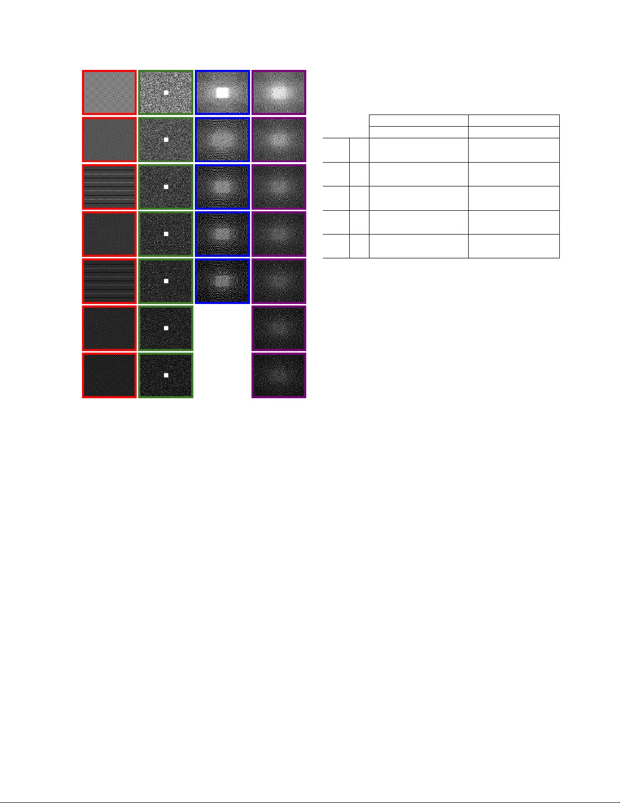
1 OEDIPUS: An Experiment Design Frame work for Sparsity-Constrained MRI Justin P . Haldar , Senior Member , IEEE, and Daeun Kim, Student Member , IEEE Abstract —This paper introduces a new estimation-theoretic framework for experiment design in the context of MR image reconstruction under sparsity constraints. The new framework is called OEDIPUS (Oracle-based Experiment Design for Imaging Parsimoniously Under Sparsity constraints), and is based on combining the constrained Cram ´ er -Rao bound with classical experiment design techniques. Compared to popular random sampling approaches, OEDIPUS is fully deterministic and au- tomatically tailors the sampling pattern to the speciﬁc imaging context of interest (i.e., accounting f or coil geometry , anatomy , image contrast, etc.). OEDIPUS-based experiment designs are evaluated using retrospectiv ely subsampled in vivo MRI data in several differ ent contexts. Results demonstrate that OEDIPUS- based experiment designs have some desirable characteristics relati ve to con ventional MRI sampling approaches. Index T erms —Experiment Design; Constrained MRI Recon- struction; Sparsity Constraints; Compressed Sensing; I . I N T RO D U C T I O N Slow data acquisition speed is a natural consequence of acquiring MRI data with high signal-to-noise ratio (SNR), high spatial resolution, and desirable image contrast characteristics. Slow acquisitions are problematic because they are expensiv e, limit scanner throughput and temporal resolution, and can be uncomfortable for scan subjects. In practice, these concerns lead to the use of shorter-duration experiments that represent undesirable trade-offs between image resolution and contrast when data is sampled according to the con ventional sampling theorem [1]. T o mitigate this problem, the research community has been working for decades to develop image reconstruction methods that enable conv entional sampling requirements to be relaxed [2]. While many such image reconstruction methods hav e been proposed ov er the years, this paper focuses on a popular and widely-used class of methods based on sparsity constraints [3]. While successful applications of sparsity-constrained MRI are widespread throughout the literature, the optimal design of sampling patterns remains a longstanding open problem. Because there is already a large amount of literature on this topic, it w ould be impractical for us to comprehensiv ely revie w ev ery contribution. Instead, our literature revie w focuses only on what we believ e is the most relev ant previous work. J. Haldar and D. Kim are with the Signal and Image Processing Institute, Ming Hsieh Department of Electrical Engineering, Univ ersity of Southern California, Los Angeles, CA, 90089, USA. This work was supported in part by the National Science Foundation (NSF) under CAREER award CCF-1350563 and the National Institutes of Health (NIH) under grants NIH-R21-EB022951, NIH-R01-MH116173, NIH-R01-NS074980, and NIH-R01-NS089212. Computation for some of the work described in this paper was supported by the Uni versity of Southern California’ s Center for High-Performance Computing (http://hpcc.usc.edu/). Some of the earliest sparsity-based methods sample low- resolution data at the con ventional Nyquist rate, and use spar- sity constraints to recov er the unsampled high-frequency data and enable super-resolution reconstruction [4]. More recently , insight pro vided by compressed sensing theory has inspired the emergence and popularity of pseudo-random Fourier sampling schemes [5]. Random Fourier sampling for MRI has often been moti vated by theoretical performance guarantees for random sampling that depend on mathematical concepts of incoherence and/or restricted isometry [6], [7]. Within the MRI community , a fairly common misconception is that random sampling is required for good sparsity-constrained MRI. In reality , random Fourier sampling is neither necessary nor sufﬁcient for good performance [5], [8], [9], particularly in the case of multi- channel imaging for which the reconstruction problem is often not actually underdetermined (and is instead just ill-posed). Most modern approaches have come to rely on heuristic vari- ations of random F ourier sampling that are often tuned for each new application context based on extensi ve empirical trial- and-error testing [5], [10]–[12]. While these kinds of random sampling v ariations often work adequately well, their good performance is not guaranteed from a theoretical perspecti ve [8], empirical tuning of random sampling characteristics is often onerous, and it remains unclear whether the results are near-optimal. This paper describes a principled method called OEDIPUS (Oracle-based Experiment Design for Imaging Parsimoniously Under Sparsity constraints) for designing sampling patterns for sparsity-constrained MRI. Compared to randomization-based approaches, OEDIPUS is fully deterministic and automatically tailors the sampling pattern to the speciﬁc imaging context (ac- counting for coil geometry , anatomy , image contrast, etc.) of interest without the need for manual interaction. A preliminary description of this work was previously presented in [13]. The OEDIPUS framew ork is inspired by classical ex- periment design approaches. Experiment design is a well- dev eloped subﬁeld of statistics [14]–[16], and experiment de- sign tools hav e been previously used to improv e the ef ﬁciency of a wide variety of MRI experiments. These methods are perhaps most visible within the MRI literature in the context of selecting ﬂip angles, repetition times, echo times, and related pulse sequence parameters that inﬂuence image contrast. Such methods hav e already had a major impact in the context of quantitativ e MRI parameter estimation for applications such as spectroscopy [17], water-f at separation [18], dynamic contrast enhanced imaging [19], diffusion MRI [20], relaxometry [21], and multi-parametric mapping [22], among many others. Howe ver , the use of experiment design techniques to op- 2 timize k-space sampling patterns (as done in OEDIPUS) has not been as widely explored, in part due to the computational complexity of applying experiment design techniques to image reconstruction problems (which are often substantially larger in scale than MRI parameter estimation problems). There are a few notable e xceptions. Marseille et al. [23] performed optimization of phase encoding positions in 1D under a heuristic surrogate model of an MR image. Reev es et al. [24]– [28] optimized phase encoding positions in 2D assuming that the image had limited support in the spatial domain, with perfect a priori knowledge of the image support, while later authors explored a similar approach in the context of dynamic imaging [29]. Xu et al. [30] performed optimization of phase encoding positions in 1D for the case of parallel imaging using the SENSE model [31]. Samsonov [32] optimized the projection angles for radial imaging under the SENSE model. Haldar et al. [33] compared different spatiotemporal (k- t) sampling patterns for parameter mapping in the presence of prior kno wledge of the image contrast model. Levine and Hargreav es [34] optimized 2D sampling patterns under support constraints and parallel imaging constraints with the SENSE model. Importantly , none of these approaches directly incorporated transform domain sparsity constraints into the experiment design problem. The only previous sparsity-based MR experiment design work we are aware of is by Seeger et al. [35]. While this work has the strongest similarity to OEDIPUS among existing methods from the literature, it also has substantial differences, including being de veloped with a completely different context in mind. In particular , the approach described by Seeger et al. is intended for real-time adaptive sampling design, in which each subsequent k-space sampling location is chosen greedily on-the-ﬂy using real-time feedback from the data that has already been acquired for that scan. In contrast, OEDIPUS is a non-adaptiv e and subject-independent approach to experiment design, which enables ofﬂine prior computation of the sampling pattern and reuse of the same sampling scheme for different subjects. Another major difference is that Seeger et al. assume a Bayesian formulation in which the sparse image coefﬁcients are modeled using the Laplace distribution as a statistical prior , while OEDIPUS is a non- Bayesian approach that does not use any statistical priors. Instead, OEDIPUS takes a deterministic approach based on the constrained Cram ´ er-Rao bound (CRB) [36], [37]. The rest of this paper is organized as follows. Section II introduces notation, revie ws the CRB for linear inv erse prob- lems with Gaussian noise, and revie ws optimal experiment design approaches that aim to minimize the CRB. Section III describes the general OEDIPUS framework as an extension of the methods from Section II. This section also describes the speciﬁc OEDIPUS implementation choices we have used in the remainder of the paper . Section IV describes empirical ev aluations of OEDIPUS with comparisons against other com- mon k-space sampling methods from the literature. Discussion and conclusions are presented in Section V. I I . R E V I E W O F “ C L A S S I C A L ” E X P E R I M E N T D E S I G N A. Linear Inver se Pr oblems with Gaussian Noise The data acquisition process in MRI is often formulated using a standard ﬁnite-dimensional linear model [38] d = Af + n , (1) where f ∈ C N are the coefﬁcients of a ﬁnite-dimensional representation of the image, d ∈ C M is the vector of measured data samples, the system matrix A ∈ C M × N provides a linear model of the MRI data acquisition physics (e.g., potentially including Fourier encoding, sensitivity encoding, and physical effects like ﬁeld inhomogeneity), and n ∈ C M is modeled as zero-mean circularly-symmetric complex Gaussian noise. W ithout loss of generality , we will assume that noise whitening has been applied such that the entries of n are assumed to be independent and identically distributed with v ariance σ 2 = 1 . The objectiv e of MRI reconstruction methods is to estimate the original image f based only on the noisy measured data d and prior knowledge of the noise statistics and imaging model A . W e will denote such an estimator as ˆ f ( d ) . B. The Cram ´ er-Rao Bound for the Linear Model The CRB is a theoretical lower bound on the covariance of an unbiased estimator [39]. Assume for no w that data has been acquired according to Eq. (1), that A has full-column rank, and that we ha ve an unbiased estimator ˆ f ( d ) , i.e., E [ ˆ f ( d )] = f , where E [ · ] denotes statistical expectation. The CRB says that co v( ˆ f ( d ))  ( A H A ) − 1 , (2) where cov( ˆ f ( d )) ∈ C N × N is the cov ariance matrix of the estimator ˆ f ( d ) , and the  symbol is used to signify an inequality relationship with respect to the Loewner ordering of positiv e semideﬁnite matrices [16]. T o be precise, Eq. (2) signiﬁes that cov( ˆ f ( d )) − ( A H A ) − 1 will always be a positiv e semideﬁnite matrix. As a result, the CRB matrix ( A H A ) − 1 represents the smallest possible cov ariance matrix that can be achiev ed using an unbiased estimator, since we must always hav e that u H co v( ˆ f ( d )) u ≥ u H ( A H A ) − 1 u for e very possible choice of u ∈ C N . T o illustrate the importance of this relationship, consider the case where we select u to be the j th canonical basis vector for C N , i.e., the j th entry of u is [ u ] j = 1 , with [ u ] n = 0 for all n 6 = j . This implies that v ar  [ ˆ f ( d )] j  ≥  ( A H A ) − 1  j j , where v ar([ ˆ f ( d )] j ) is the scalar v ariance of the estimator for the j th entry of f . Note that, because we ha ve chosen j arbitrarily in this illustration, we hav e that the N diagonal elements of the CRB matrix each provide a fundamental lo wer bound on the v ariance for the corresponding N entries of the unbiased estimator ˆ f ( d ) . Importantly , the CRB is a function of the matrix A , which means that it can be possible to use the CRB to compare the SNR-efﬁcienc y of dif ferent e xperiments. For readers familiar with the parallel MRI literature, it is worth mentioning that in the case of SENSE reconstruction, the CRB is an unnormal- ized version of the SENSE g-factor [31], [40], which is already well kno wn and widely used for its usefulness in comparing different k-space sampling strategies in parallel MRI. 3 In addition, the CRB is a reconstruction-agnostic lo wer bound, in the sense that it is completely independent from the actual method used to estimate f . Howe ver , it should also be noted that the CRB is only valid for unbiased estimators, while different estimation-theoretic tools are necessary to characterize biased estimators. This fact is particularly rele vant to this paper, since most sparsity-constrained reconstruction methods use some form of regularization procedure, and regularized image reconstruction will generally produce biased results [41]. Nev ertheless, minimizing the CRB can still be a useful approach to experiment design e ven if a biased estimator will ultimately be used for reconstruction. In some sense, minimizing the CRB ensures that the data acquisition procedure represented by the matrix A will encode as much information as possible about f . C. Optimal Experiment Design using the CRB Methods for minimizing the CRB have been studied for many years in both statistics [14]–[16] and signal processing [42], [43]. There are generally two classes of popular exper- iment design approaches: continuous approaches and discrete approaches. Optimal continuous designs are often easier to compute than optimal discrete designs, but are approximate in nature and do not translate easily to the constraints of practical MRI experiments because they do not account for the fact that real experiments acquire a ﬁnite, integer number of samples. As a result, we will focus on discrete designs in this paper . The discrete version of optimal experiment design is often formulated as follows: gi ven a set of P candidate measure- ments (with P > M ), choose a subset of M measurements in a way that minimizes the CRB. Formally , let a p ∈ C 1 × N for p = 1 , . . . , P represent the P potential rows of the optimal A matrix from Eq. (1). Giv en the corresponding set of potential measurement indices Γ = { 1 , . . . , P } , the optimal design problem is to select a subset Ω ⊂ Γ of cardinality M to ensure that the resulting CRB is as small as possible. This leads to the optimal design problem Ω ∗ = arg min Ω ⊂ Γ | Ω | = M J   X m ∈ Ω a H m a m ! − 1   , (3) where J ( · ) : C N × N → R is a user-selected functional used to measure the size of the CRB. An ideal choice of J ( · ) would ensure that for arbitrary positiv e semideﬁnite matrices C ∈ C N × N and D ∈ C N × N , having J ( C ) ≥ J ( D ) would imply that C  D , and therefore that D is uniformly smaller than C . Unfortunately , the Loe wner ordering is only a partial ordering, and not all positiv e semideﬁnite matrices are comparable. This means that there are generally no univ ersally-optimal experiment designs, and it is necessary to choose J ( · ) subjectiv ely [16]. Out of many options [16], one of the most popular choices is the averag e variance criterion (also known as A-optimality ): J   X m ∈ Ω a H m a m ! − 1   , T race   X m ∈ Ω a H m a m ! − 1   , (4) which takes its name from the fact that the cost function is a lower bound on the sum of elementwise variances, i.e., T race   X m ∈ Ω a H m a m ! − 1   ≤ N X n =1 v ar([ ˆ f ( d )] n ) (5) for every possible unbiased estimator ˆ f ( d ) . Since the mean- squared error (MSE) is proportional to the sum of elementwise variances for any unbiased estimator , Eq. (5) also provides a CRB-based lower bound for the MSE. For the sake of concreteness and without loss of generality , we will focus on the A-optimality criterion in this paper , though note that OEDIPUS can also easily be used with some of the other cost functionals that are popular in the experiment design literature. Giv en this choice of J ( · ) , the optimization problem from Eq. (3) is still nontrivial to solve because it is a noncon ve x integer programming problem, and global optimality may re- quire exhausti ve search through the set of candidate solutions. This is generally infeasible from a practical computational per- spectiv e. Speciﬁcally , there are P -choose- M possible designs Ω , and this will be a very large number in most scenarios of interest. As a result, Eq. (3) is often minimized using heuristic algorithms that can provide high-quality solutions, but which cannot guarantee global optimality . Popular heuristics include the use of Monte Carlo methods (which randomly construct potential sampling pattern candidates for e valuation) or greedy algorithms (which add, subtract, or exchange candidate mea- surements to/from the current design in a sequential greedy fashion) [14], [15], [42], [43]. While these kinds of algorithms hav e been used previously for k-space trajectory design in se veral image reconstruction contexts [24]–[28], [30], certain computational problems arise when the CRB is applied to con ventional image reconstruction approaches (without sparsity constraints). In particular, the CRB matrix is of size N × N , which can be very large if N is chosen equal to the number of voxels in a reasonably-sized image. For example, for a 256 × 256 image, the CRB matrix will hav e nearly 4 . 3 × 10 9 entries, which will occupy more than 34 GB of memory if each entry is stored in a standard double precision ﬂoating point number format. While storing a matrix of this size in memory is feasible on modern high-end computers, other computations (e.g., inv erting the matrix) are generally prohibitively expensi ve. Another problem is that the assumptions underlying the CRB will be violated whenever N > M , which means that traditional experiment design approaches are not straightforward to apply for the design of undersampled experiments. These issues are mitigated within the OEDIPUS framew ork as described in the sequel. I I I . O R A CL E - B A S E D E X P E R I M E N T D E S I G N F O R I M AG I N G P A R S I M O N I O U S L Y U N D E R S PA R S I T Y C O N S T R A I N T S A. Theoretical components of OEDIPUS The previous section considered CRB-based design under the standard unconstrained linear model, but modiﬁcations are necessary to inform experiment design under sparsity constraints. T o describe OEDIPUS, we will assume that it is known in advance that the image vector f possesses a 4 certain lev el of sparsity in a known transform domain, i.e., k Ψf k 0 ≤ S where Ψ ∈ C Q × N is a kno wn sparsifying transform, S is the known sparsity le vel, and the ` 0 -“norm” k · k 0 counts the number of nonzero entries of its vector argument. It should be noted that the assumptions that the signal is strictly sparse and that the v alue of S is known in advance are not conv entional in sparsity-constrained MRI reconstruction, though we need them to construct the CRB for this case. In this work, we will make the additional assumption that Ψ is left-in vertible such that f = Ψ † Ψf for all f ∈ C N , where † is used to denote the matrix pseudoinv erse. In the presence of sparsity constraints, this allows us to rewrite Eq. (1) in terms of the vector of transform coefﬁcients c = Ψf ∈ C Q as: d = AΨ † c + n . (6) Recently , Ben-Haim and Eldar [37] derived a version of the constrained CRB that is applicable to Eq. (6) under the constraint that k c k 0 = S . In particular , they deriv ed that the CRB in this case is equal to the CRB of the oracle estimator , i.e., the estimator that is additionally bestowed with perfect knowledge of which of the S entries of c are non-zero. The oracle-based version of the problem can be viewed as a simple unconstrained linear model, and thus ﬁts directly within the framework described in the previous section. In particular, let ˜ c ∈ C S denote the vector of nonzero entries from the c vector , with the two vectors related through c = U ˜ c , where U ∈ R Q × S is a matrix formed by concatenating the S columns of the Q × Q identity matrix corresponding to the non-zero entries of c . This matrix can be viewed as performing a simple zero-ﬁlling operation (i.e., putting the nonzero entries of ˜ c in their correct corresponding positions and lea ving the remaining entries equal to zero). Giv en this notation, the oracle-based version of the problem is then written as d = AΨ † U ˜ c + n . (7) From here, we can use the results of the previous section to easily deriv e the oracle-based CRB for ˆ ˜ c ( d ) : co v( ˆ ˜ c ( d ))   U H  Ψ †  H A H AΨ † U  − 1 , (8) such that the oracle-based CRB for ˆ c ( d ) = U ˆ ˜ c ( d ) is: co v( ˆ c ( d ))  U  U H  Ψ †  H A H AΨ † U  − 1 U H , (9) and the oracle-based CRB for ˆ f ( d ) = Ψ † ˆ c ( d ) is: co v( ˆ f ( d ))  Ψ † U  U H  Ψ †  H A H AΨ † U  − 1 U H  Ψ †  H . (10) Giv en these sparsity-constrained CRBs, it is easy to formulate and solve an experiment design problem using exactly the same design methods described for the linear model in the previous section. The CRB expressions gi ven abov e will be valid whene ver the M × S matrix AΨ † U has full column rank, which is still feasible for undersampled experiments where M < N (though we still need to satisfy S ≤ M ). In addition to enabling the use of sparsity constraints and undersampling in experiment design, the expressions in Eqs. (8)-(10) are generally also substantially easier to work with from a computational point of view . In particular, it should be noted that the matrices being in verted in these expressions are only of size S × S , rather than the N × N matrices that needed to be in verted in the pre vious case. This can lead to massive computational comple xity advantages since we usually hav e S  N . F or example, for a 256 × 256 image with S = 0 . 15 N , the matrix to be inv erted in this case would have roughly 2.25% the memory footprint of the matrix to be in verted in the N × N case. In this example, this is the difference between a 0.8 GB matrix and a 34 GB matrix. Even though the ﬁnal CRB matrices in Eqs. (9) and (10) are generally larger (respectively of size Q × Q and N × N ) than the S × S matrix being inv erted in Eq. (8), it is not hard to show that the matrices in Eqs. (8) and (9) always hav e the same trace value. In addition, the trace value for the matrix from Eq. (10) will also hav e this same trace value if Ψ is a unitary transform (e.g., an orthonormal wavelet transform) and will be proportional to this same trace v alue if Ψ corresponds to a tight frame representation [44] (e.g., the undecimated Haar wa velet transform [45] or the discrete curvelet transform [46]). As a result, it often suf ﬁces to work directly with the small S × S matrix from Eq. (8) when performing experiment design using the A-optimality design criterion. B. Practical Implementation for MRI Applications 1) Constructing the OEDIPUS optimization problem: For the sake of concreteness and without loss of generality , we will describe our implementation of OEDIPUS assuming that we are applying the A-optimality design criterion to the sparsity- constrained CRB from Eq. (8). Giv en an application context, there are sev eral ingredients we need to select prior to the experiment design process. The ﬁrst choice that needs to be made is the sparsifying transform Ψ . While some groups have explored the use of data-dependent sparsifying transforms (e.g., [47], [48]), it is by far more common for the sparsifying transform to be chosen in advance based on past empirical experience with a giv en MRI application. Our description will focus on the conv entional case where Ψ is ﬁxed and provided in advance. The second choice we need to make relates to the set of candidate measurement vectors a p ∈ C 1 × N for p = 1 , . . . , P . This choice is relativ ely straightforward in the case of ideal single-channel Fourier encoding. Given a ﬁeld-of-vie w (FO V) size and the number of vox els within the FO V (which we assume are ﬁxed, and dictated by the speciﬁc application context of interest), the candidate measurement vectors will often have entries (assuming an N -dimensional voxel-based ﬁnite series expansion of the image [38]) of the form: [ a p ] 1 n = b pn exp( − i 2 π k p · r n ) , (11) where b pn is a weighting coefﬁcient that depends on the speciﬁc choice of voxel basis function (common choices are to use either a Dirac delta vox el function in which b pn = 1 or a rectangular voxel basis function in which case b pn takes the 5 form of a sinc function in k-space [38]), r n is the spatial coordinate vector specifying the center position of the n th vox el (the common choice is to choose the voxel centers to lie on a rectilinear grid), and k p is the p th candidate k- space measurement position. The parameters b pn and r n are parameters of the image model that are generally chosen in advance, and which will be in variant to dif ferent experiment design choices. As a result, selection of the full set of the candidate measurements reduces to selection of the set of k p k-space sampling locations. The set of candidate k-space sampling locations will be sequence dependent, but typical choices might include the set of all possible k-space sampling locations from a “fully-sampled” Cartesian grid, a “fully- sampled” radial trajectory , a “fully-sampled” spiral trajectory , etc. In each of these cases, we can deﬁne “full-sampling” either based on the con ventional Nyquist rate, or we can also consider schemes that sample more densely than the Nyquist rate if we want to consider a larger range of possibilities. There is a trade-off here – the more options we consider, the better our optimized schemes can be, though this comes at the expense of increased computational comple xity . Some additional considerations are required if the model is designed to incorporate sensiti vity encoding, ﬁeld inhomo- geneity , radiofrequency encoding, or other similar ef fects. For illustration, in the case of parallel imaging with the SENSE model [31], the measurements take the more general form: [ a p ] 1 n = c p ( r n ) b pn exp( − i 2 π k p · r n ) , (12) where c p ( r n ) is the v alue of the sensitivity proﬁle at spatial location r n for the coil used in the p th measurement. 1 The main complication in applying OEDIPUS to the SENSE model is that, while the Fourier encoding model is independent of the person or object being imaged, the coil sensitivity proﬁles often vary slightly from subject to subject, and this means that ideally we should design optimal experiments on a subject-by-subject basis. Howe ver , subject-by-subject design is not conducive to the kind of ofﬂine subject-independent experiment design that we would like to use OEDIPUS to address. Similar complications exist because of subject- dependent effects for other advanced modeling schemes that account for B 0 inhomogeneity , transmit B 1 inohomogeneity , etc. T o mitigate the issue of subject-dependent observations, our formulation for the SENSE case (and similarly for other subject-dependent acquisition models) will assume that we hav e a set of T different representati ve sensitivity maps that are appropriate for the given application context, i.e., [ a t p ] 1 n = c t p ( r n ) b pn exp( − i 2 π k p · r n ) , (13) for t = 1 , . . . , T , and will optimize the experiment design with respect to the ensemble of these representative cases. W e will formalize this approach mathematically later in this section. The remaining ingredients that need to be chosen are the sparsity lev el S and the matrix U that speciﬁes the transform- domain positions of the non-zero coefﬁcients. Howe ver , real 1 In parallel MRI, the same k-space location is measured simultaneously through all of the coils that are present in the receiv er array . W e have adopted a notation in which each individual measurement is indexed by a separate p value, even if some measurements are required to be sampled simultaneously . MRI images are only approximately sparse rather than exactly sparse, and the locations of the signiﬁcant transform-domain coefﬁcients will generally vary from subject to subject. T o address these issues and enable subject-independent experi- ment design, we will assume that we are giv en a set of K ex emplar images acquired from a giv en imaging context, and similar to the pre vious case, will identify S k and U k values for k = 1 , . . . , K that are appropriate for each case. Ultimately , we will attempt to ﬁnd a design that is optimal with respect to the ensemble of exemplars. In this context, we ﬁrst apply the sparsifying transform Ψ to each exemplar , and explore sparse approximation quality by hard-thresholding the transform do- main coefﬁcients with different choices of S k . The value of S k is then chosen as the smallest value that gi ves adequate sparse approximation quality for that exemplar . Note that “adequate quality” is necessarily subjective and application dependent. Giv en the choice of S k for each ex emplar image, we can obtain corresponding U k ∈ R Q × S k matrices by identifying the locations of the S k largest transform coefﬁcients. W e are now almost ready to perform experiment design, except that we have not speciﬁed how to handle optimization with respect to the ensemble of T different measurement models and K different ex emplar sparsity constraints. There are a few dif ferent options for obtaining a uniﬁed treatment. One typical approach would be to minimize the average-case CRB across each of these different conditions, which results in the following optimization problem: Ω ∗ = arg min Ω ⊂ Γ | Ω | = M K X k =1 T X t =1 T race [ C kt (Ω)] , (14) where C kt (Ω) , X m ∈ Ω U H k  Ψ †  H ( a t m ) H a t m Ψ † U k ! − 1 . (15) Another typical choice would be to optimize the worst-case CRB, which leads to the following minimax optimization problem: Ω ∗ = arg min Ω ⊂ Γ | Ω | = M max ( k,t ) T race [ C kt (Ω)] . (16) Many other choices are also possible and may be preferable in certain contexts, though we lea ve such an exploration for future work. The choice between minimizing the av erage-case and the worst-case in e xperiment design is subjecti ve in nature, and will depend on context-dependent factors. For example, in a large population study with a neuroscientiﬁc objectiv e, experimenters may be able to tolerate the situation where a few subjects hav e low-quality images if the average image quality for the remaining subjects is very high on av erage. On the other hand, in an emergency medical situation, it may be preferable that every individual image meets certain quality standards, ev en if that means that the average-case image quality is lower as a result. In the case where K = T = 1 , both Eq. (14) and (16) lead to identical optimization problems. 6 2) Solving the OEDIPUS optimization pr oblem: Giv en a choice of objective function, it remains to ﬁnd an experiment design that is as close to optimal as possible. While there are many potential ways to minimize these cost functionals, the implementation we hav e used for this paper is based on a modiﬁed sequential backward-selection (SBS) procedure. The standard SBS procedure [42], [43] starts with a hypothetical experiment that collects all P candidate measurements, and then identiﬁes the individual measurement that is the least important to the CRB and deletes it in a greedy fashion. This procedure is then iterated, deleting candidate measurements one-by-one until only M measurement vectors remain. SBS is greedy and will not generally ﬁnd the globally optimal solu- tion, b ut it is a simple deterministic algorithm that typically ob- tains local minima that compare very well in ultimate quality compared to alternativ e optimization approaches. Additional theoretical comments about the characteristics of SBS can be found in [42], and methods that ha ve the potential to improve on SBS results are discussed in [43]. While the con ventional SBS approach may be well-suited to certain applications, it is not immediately applicable to many MRI contexts in which sets of measurements must be acquired simultaneously . For example, in parallel imaging, it does not make any sense to delete a k-space measurement made with one coil without also deleting the same k-space measurement from the remaining coils. Similarly , it would not make sense to delete one k-space measurement from a giv en readout without also deleting the other measurements from the same readout. As a result, it is important to be able to adapt SBS to consider sets of candidate measurements rather than individual candidate measurements. Speciﬁcally (and similar to [27], [28], [30]), we will assume that our set of P measurements is grouped into L disjoint subsets Ξ ` for ` = 1 , . . . , L , and that all measurements within a giv en subset Ξ ` must either be acquired simultaneously or not acquired at all. W e will further assume the practical scenario in which all of these measurement sets have the same cardinality , i.e., | Ξ ` | = C for some integer C . This leads to the follo wing modiﬁed SBS procedure for OEDIPUS: 1) For k = 1 , . . . , K and t = 1 , . . . , T , construct the sparsity-constrained CRB matrix corresponding to the use of all P candidate measurements: C full kt = P X p =1 U H k  Ψ †  H ( a t p ) H a t p Ψ † U k ! − 1 . (17) As noted in Sec. III-A, this matrix is often not very large (i.e., of size S × S ), and will therefore ﬁt easily within the memory capacities of most modern computers if S is chosen suitably small. 2) For each ` = 1 , . . . , L , compute the cost-function value (e.g., the average-case cost from Eq. (14) or the worst- case cost from Eq. (16)) for an experiment that uses all P measurements except the C candidate measurements included in Ξ ` . 3) The cost-function v alues are compared for each choice of ` , and the measurement set whose remov al causes the smallest degradation in the cost function v alue is then remov ed from the set of measurement candidates. Speciﬁcally , if i is the index for the removed set of mea- surement candidates, set Γ = Γ \ Ξ i , and correspondingly set P = P − C . Similarly , remov e Ξ i from the set of measurement candidates such that L = L − 1 . 4) Repeat Steps 1-3 until the desired number of measure- ments is achiev ed, i.e., stop when | Γ | = M . The main computational complexity associated with this modiﬁed SBS approach is that Step 2 requires T LK matrix in versions at each iteration. Howe ver , as thoroughly discussed by [42], it should be noted that it is easy and computationally- efﬁcient to use the Sherman-Morrison-W oodbury matrix in- version lemma [49] to use the matrix from Step 1 to quickly compute the matrices needed for Step 2. Speciﬁcally , if we use B `t ∈ C C × N to denote the matrix formed by stacking together the potential rows associated with Ξ ` for the t th acquisition model and let ˜ B k `t = B `t Ψ † U k ∈ C C × S , then the CRB matrix C full \ Ξ ` kt that would be obtained by keeping all P measurements except those from Ξ ` can be written as C full \ Ξ ` kt =     P X p =1 p / ∈ Ξ ` U H k  Ψ †  H ( a t p ) H a t p Ψ † U k     − 1 = C full kt + G k `t  I C − ˜ B k `t G k `t  − 1  G k `t  H , (18) where I C is the C × C identity matrix and G k `t = C full kt  ˜ B k `t  H . Note that this ﬁnal expression only requires the in version of a C × C matrix, which is a much faster computation than inv erting an S × S matrix if C  S (which it usually will be). In addition, it should be noted that e xcept for the ﬁrst time that C full kt is computed using Eq. (17) in Step 1, all subsequent computations of C full kt for Step 1 can be performed recursively from the previous value using Eq. (18). Further computational simpliﬁcations are possible by noting that the trace v alues required for computing Step 2 are also easily ev aluated in a recursi ve fashion: T race h C full \ Ξ ` kt i = T race  C full kt  + T race  G k `t  I C − ˜ B k `t G k `t  − 1  G k `t  H  . (19) I V . E M P I R I C A L E V A L U A T I O N S A N D C O M P A R I S O N S In the following subsections, we illustrate the performance and ﬂexibility of OEDIPUS relativ e to traditional sampling design methods in sev eral settings. A. 2D T2-weighted Br ain Imaging In a ﬁrst set of ev aluations, we designed sampling patterns for the context of 2D T2-weighted brain imaging, based on an acquisition protocol that is routinely used at our neuroscience imaging center . Data was acquired on the same scanner from sev en different healthy volunteers on different days. All acquisition parameters were identical for all subjects. Imaging data was acquired with a TSE pulse sequence on a 7 (a) Magnitude (b) Phase (c) W avelet Fig. 1. Gold standard reference images for the 2D T2-weighted brain imaging experiment. The top row shows data from the ﬁrst subject, while the bottom row shows data from the second subject. 3T scanner using a 12-channel receiver coil. W e used a fully- sampled 256 × 160 Nyquist-rate Fourier acquisition matrix, corresponding to a 210mm × 131mm FO V , with a 3.5mm slice thickness. Other parameters include TE=88ms and TR=10sec. This data was whitened using standard methods [50], and re- ceiv er coil sensitivity maps were obtained using a smoothness- regularized estimation formulation [51]. Gold standard refer- ence images were obtained by applying SENSE reconstruction [31], [50] to the fully sampled data. These gold standard images for two subjects are shown in Fig. 1(a,b). Sampling patterns were designed using OEDIPUS for two different imaging scenarios: single-channel imaging (a sim- ple Fourier transform with no sensitivity encoding) and 12- channel imaging (including coil sensitivity maps). In both cases, the design was performed with respect to a single slice for simplicity , although it would ha ve been straightforward to use volumetric training data (or , to reduce computational complexity , perhaps a small number of selected slices rep- resenting the range of expected v ariations across the volume of interest) for cases where broader volume coverage may be desired. W e denote the OEDIPUS sampling patterns designed for the single-channel and multi-channel cases as SCO and MCO, respectively . Since this is a 2D imaging scenario, OEDIPUS was constrained so that all samples from the same readout line must be sampled simultaneously , meaning that undersampling was only performed in 1D along the phase encoding dimension. For illustration (and without loss of generality), we show OEDIPUS sampling patterns that were designed for a single examplar (i.e., K = 1 ), and in the multi-channel case, for a single set of sensitivity maps (i.e., T = 1 ). Speciﬁcally , OEDIPUS was performed based on the transform-domain sparsity pattern and sensitivity maps estimated from the ﬁrst subject. Sparse approximation of this dataset was obtained by keeping the top 15% largest-magnitude transform coefﬁcients (i.e., S = 0 . 15 N ). The sparsifying transform Ψ was chosen to be the 3-le vel wav elet decomposition using a Daubechies- 4 wav elet ﬁlter, whose transform coefﬁcients are shown for the ﬁrst two subjects in Fig. 1(c). As can be seen, while the images and the exact distributions of wavelet coefﬁcients are distinct for each of the two datasets, the wav elet-domain support patterns for both images still have strong qualitative similarities to one another . This similarity is one of the key assumptions that enables OEDIPUS to design sampling patterns based on exemplar data instead of requiring subject- speciﬁc optimization. MCO sampling patterns were designed for the acceleration factors of R = 2 , 3, and 4, and an SCO sampling pattern was designed for R = 2 . W e also attempted to design SCO sampling patterns for the acceleration factors of R = 3 and 4, but did not obtain meaningful OEDIPUS results because the matrix inv ersions needed for computing the CRB became numerically unstable. This instability occured because the matrices became nearly-singular , which is an indication that acceleration factors of 3 or 4 may be too aggressi ve for unbiased estimation in this particular scenario. Speciﬁcally , near-singularity implies that unbiased estimators would have very large v ariance for certain parameters of interest (i.e., a singular matrix is associated with inﬁnite variance [52]). This is consistent with our empirical results (not sho wn due to space constraints) for which R = 3 or 4 yields unacceptably poor results in this scenario for every case we attempted. For comparison against SCO and MCO, we also consid- ered tw o classical undersampling patterns: uniform under- sampling and random undersampling. Uniform undersampling is a deterministic sampling pattern that is frequently used in parallel imaging [31], and obtains phase encoding lines that are uniformly spaced on a re gular lattice in k-space. Random sampling is often advocated for sparsity-constrained reconstruction [5], [8], [10]–[12]. In this case, we used a common approach in which the central 16 lines of k-space were fully sampled, and the remaining portions of k-space were acquired with uniform Poisson disc random sampling [53]. It is worth mentioning that both the uniform and random sampling schemes considered in this work are expected to be better-suited to multi-channel scenarios than they are to single- channel cases. In particular , uniform undersampling is not usually advocated in single-channel settings due to the well- known coherent aliasing associated with lattice sampling, and single-channel random undersampling usually employs a more gradual variation in sampling density rather than the abrupt binary change in sampling density that we’ ve implemented. Nev ertheless, due to the lar ge number of subjects and scenarios we consider in this paper and the effort associated with manually tuning more nuanced sampling density variations by trial-and-error , we have opted for the sake of simplicity to utilize the same type of simple random sampling design for both single- and multi-channel cases. T o av oid the possibility of getting a particularly bad random design, we created ten independently generated realizations of Poisson disc sampling, and report the best quantitative results. The sampling patterns we obtained are shown in Fig. 2, and demonstrate some interesting features. In particular , we observe that both SCO and MCO generate variable density 8 Uniform Random SCO MCO R = 2 R = 3 R = 4 Fig. 2. Sampling patterns for the 2D T2-weighted brain imaging experiment. sampling patterns, which is consistent with the popularity of variable density sampling approaches in the literature [5], [8], [10]–[12]. Howe ver , unlike standard randomization-based variable density approaches, we observe that OEDIPUS auto- matically tailors the sampling pattern to the speciﬁc imaging context, without the need for manual interaction. This can be observed from the fact that OEDIPUS automatically produces different sampling density variations for single-channel and multi-channel contexts, with SCO sampling the center of k- space more densely than MCO. T o ev aluate these different sampling patterns in a prac- tical reconstruction context, we also performed sparsity- constrained reconstructions of retrospectively-undersampled single-channel and multi-channel datasets derived from the gold standard reference images. W e might expect to see especially good empirical reconstruction results for OEDIPUS for the ﬁrst subject, since the SCO and MCO sampling patterns were designed based on the characteristics of that data. In this case, we are testing on the same data that we trained on, and our results may be ov erly optimistic due to the common problem of overﬁtting. On the other hand, the empirical results from the other subjects may be more interesting, since these will demonstrate the capability to design sampling patterns that generalize beyond the training data. W e performed two different types of sparsity-constrained reconstruction. In the ﬁrst case, we applied standard ` 1 - regularized reconstruction [5] according to ˆ f = arg min f ∈ C N k Af − d k 2 2 + λ k Ψf k 1 . (20) This formulation will encourage sparsity in the 3-level Daubechies-4 wavelet decomposition of the image. The reg- ularization parameter λ was set to a small number (i.e., T ABLE I T A B L E O F N R MS E V A L U ES F O R R EC O N S TR UC T E D S I NG L E - C H A N N EL 2 D T 2 - W E I G HT E D B R A IN DAT A . R E SU LT S A RE S H OW N F O R W A V E L E T ( W A V ) A N D T O T A L V A R I A T I ON ( T V) R E C ON S T RU C TI O N A P P ROAC H E S , A N D F O R U N IF O R M ( U N I ) , R A N D OM ( R A N D ) , A N D O E DI P U S S A M P LI N G PA T T E RN S . First Subject (T raining) Second Subject Uni Rand SCO MCO Uni Rand SCO MCO R = 2 W av 0.792 0.178 0.126 0.310 0.855 0.204 0.143 0.339 TV 0.801 0.114 0.095 0.185 0.801 0.155 0.114 0.305 λ = 0 . 01 ) to promote data consistency . W e might expect OEDIPUS to perform particularly well in this case, because the sparsifying transform used to design SCO and MCO sampling patterns is matched to the sparsifying transform being used for reconstruction. While MR images are known to posses wa velet sparsity , it has also been observed that wav elet-based sparse regulariza- tion often results in undesirable high-frequency oscillation arti- facts. As a result, many authors (e.g., [5], [8]) have advocated the use of total variation (TV) regularization [54] to either augment or replace wa velet re gularization. TV regularization is designed to impose sparsity constraints on the ﬁnite differ- ences of a reconstructed image. Unfortunately , our OEDIPUS formulation is not easy to apply to TV regularization, because TV is not associated with a left-in vertible transform. Howe ver , some authors hav e postulated that CRB-based experiment design may still be beneﬁcial ev en in cases where the model used to compute the CRB is different from the model used for image reconstruction [23], as long as both models capture the beha vior of similar image features of interest. T o test this, we also performed TV -regularized reconstruction. Speciﬁcally , we solved the same optimization problem as in Eq. (20), but replacing the ` 1 -norm with a TV penalty while leaving the regularization parameter λ the same. In both cases, optimization was performed using a multi- plicativ e half-quadratic algorithm [55], [56] (also kno wn as “It- erativ ely Reweighted Least Squares” or “Lagged Diffusi vity”). Reconstruction quality was measured quantitati vely using the normalized root-mean-squared error (NRMSE), deﬁned as NRMSE = k ˆ f − f ∗ k 2 / k f ∗ k 2 , where f ∗ is the gold standard. The empirical NRMSE results for the reconstruction of single-channel data for the ﬁrst two subjects are shown in T a- ble I and for the remaining subjects in Supplementary T able SI, with illustrativ e reconstructed images shown in Supplementary Fig. S1, 2 while NRMSE results for the reconstruction of multi- channel data are shown for the ﬁrst two subjects in T able II and for the remaining subjects in Supplementary T able SII, with illustrativ e reconstructed images shown in Supplementary Fig. S2. For single-channel data, the SCO sampling pattern worked the best for both wavelet- and TV -based reconstruction. The differences in NRMSE between SCO and the other approaches were often substantial, with random sampling being the next best approach. Uniform undersampling had very poor per- 2 This paper has supplementary downloadable material provided by the authors, av ailable at http://ieeexplore.ieee.org in the supplementary ﬁles/multimedia tab. 9 T ABLE II T A B L E O F N R MS E V A L U ES F O R R EC O N S TR UC T E D M U L T I -C H A N NE L 2 D T 2 - W E I G HT E D B R A IN DAT A . R E SU LT S A RE S H OW N F O R W A V E LE T ( W AV ) A N D T O T A L V A R I A T I ON ( T V) R E C ON S T RU C TI O N A P P ROAC H E S , A N D F O R U N IF O R M ( U N I ) , R A N D OM ( R A N D ) , A N D O E DI P U S S A M P LI N G PA T T E RN S . First Subject (T raining) Second Subject Uni Rand SCO MCO Uni Rand SCO MCO R = 2 W av 0.046 0.051 0.056 0.049 0.053 0.061 0.065 0.056 TV 0.043 0.046 0.052 0.046 0.050 0.055 0.060 0.053 R = 3 W av 0.087 0.090 0.072 0.105 0.110 0.084 TV 0.071 0.076 0.064 0.085 0.092 0.075 R = 4 W av 0.160 0.149 0.096 0.194 0.176 0.113 TV 0.126 0.117 0.082 0.145 0.144 0.097 formance in this case, although this is unsuprising because uniform undersampling is known to be a poor choice for sparsity-constrained reconstruction of single-channel data [5]. In the multi-channel case, the MCO sampling worked the best for both wav elet- and TV -based reconstruction at high acceleration factors (i.e., R = 3 and 4). W e observed that uniform random sampling worked the best with R = 2 , although MCO follows close behind and all four sampling schemes work similarly well at this low acceleration rate. The good performance of uniform undersampling for multi-channel data at low-acceleration rates occurs despite the fact that it had a slightly worse CRB than MCO, although is consistent with theoretical g-factor arguments from the parallel imaging literature [31], [50]. W e also observe that the SCO pattern seems to work better with single-channel data and MCO works better with multi- channel data, as should be expected. In addition, our results show that the OEDIPUS sampling patterns designed for one subject generally yielded good performance when applied to similar data from other subjects. B. 3D T1-weighted Br ain Imaging In a second set of e valuations, we designed sampling patterns for the context of 3D T1-weighted brain imaging, also based on an acquisition protocol that is routinely used at our neuroscience imaging center . Data was acquired on the same scanner from one healthy volunteer and one subject with a chronic stroke lesion. The healthy volunteer was scanned more than 13 months after the stroke subject. Most acquisition parameters were identical for both sub- jects. Imaging data was acquired with an MPRA GE pulse sequence on a 3T scanner using a 12-channel receiv er coil. Along the two phase-encoding dimensions, we used a fully- sampled 156 × 192 Fourier acquisition matrix, corresponding to a 208mm × 256mm FO V . Because this FO V is much larger than necessary along the left-right dimension, all image reconstruc- tions and experiment designs were performed with respect to a 156 × 126 vox el grid corresponding to a smaller 208 mm × 168 mm FO V . The third (readout) dimension was reconstructed with 1mm resolution, and we extracted one slice along this dimension to be used in our sampling inv estigation. Other parameters include TI=800ms, TE=3.09ms, TR=2530ms, and ﬂip angle = 10 ◦ . (a) Magnitude (b) Phase (c) W avelet Fig. 3. Gold standard reference images for the 3D T1-weighted brain imaging experiment. The top ro w shows data from the healthy subject, while the bottom row shows data from the stroke subject. The slice we’ ve chosen for the stroke subject includes both a stroke lesion and a ﬁducial marker , both of which are absent in the image for the healthy subject. The ﬁducial marker appears as a white circle on the top left side of the image, while the lesion appears as a dark spot in the white matter near the middle of the brain on the left side of the image. While both datasets were acquired using the same 12- channel array coil, the data for the stroke subject had been hardware-compressed by the scanner do wn to 4 virtual chan- nels, while we had access to the original 12-channels of data for the healthy subject. T o reduce the differences in sensitivity encoding information content between the two datasets, we used standard software coil-compression methods [57], [58] to reduce the data for the healthy subject to 5 virtual channels. From the coil-compressed data, we obtained receiv er coil sensitivity maps and gold standard reference images following the same procedures as described in the pre vious section. These gold standard images are shown in Fig. 3. Similar to the previous case, we used OEDIPUS to design sampling patterns for both single-channel imaging and multi- channel imaging. Since this is a 3D imaging scenario, we ga ve OEDIPUS the freedom to undersample in 2D along both phase encoding dimensions. For illustration (and without loss of generality), OEDIPUS sampling patterns were designed using the same approach described in the previous section (i.e., K = 1 , T = 1 , S = 0 . 15 N , and using the 3-le vel Daubechies- 4 wav elet decomposition) based on the single-slice from the healthy subject. The wa velet coefﬁcients for both reference images are shown in Fig. 3(c). As before, we observ e strong qualitativ e similarities in the wa velet-domain support patterns for both images, despite the presence of a lesion in one image but not in the other . MCO and SCO sampling patterns were both designed for sev eral acceleration factors between R = 2 and 8. Compared to the previous case, the use of 2D undersampling instead of 1D undersampling enables higher acceleration factors for SCO, although high ill-posedness still prevented us from computing meaningful SCO results for R = 7 and 8. Similar to the previous case, we compared SCO and MCO sampling designs against uniform and random sampling. For uniform undersampling, we used CAIPI-type uniform lattice sampling designs that are kno wn to hav e good parallel imaging 10 Uniform Random SCO MCO R = 2 R = 3 R = 4 R = 5 R = 6 R = 7 R = 8 Fig. 4. Sampling patterns for the 3D T1-weighted brain imaging experiment. characteristics [59]. For random sampling, we used a standard approach in which the central 16 × 16 re gion of k-space was fully sampled, and the remaining portions of k-space were acquired with uniform Poisson disc random sampling. As before, we created ten independently generated realizations of Poisson disc sampling, and report the best results. The sampling patterns we obtained are sho wn in Fig. 4. Sim- ilar to the pre vious case, we observe that both SCO and MCO generate variable density sampling patterns, but that SCO and MCO ha ve v ery different sampling density characteristics from one another . In particular, SCO frequently samples the center of k-space more densely than MCO does, while MCO samples peripheral k-space more densely than SCO. Interestingly , we observe that SCO with R = 2 performs full sampling of central k-space. Because the k-space acquisition grid was designed for a larger FO V while reconstruction is performed ov er a smaller FO V , this corresponds to oversampling the center of k-space (i.e., at a rate higher than the conv entional Nyquist rate). On the other hand, at higher acceleration factors, we observe that both the SCO and MCO approaches sample the center of k-space less densely than conv entional variable- density random sampling schemes (where the center of k- space is frequently sampled at the Nyquist rate) that are popular for sparsity-constrained MRI. In addition, the SCO pattern visually appears to have more structure than is typical in random designs. This illustrates the fact that not only is T ABLE III T A B L E O F N R MS E V A L U ES F O R R EC O N S TR UC T E D S I NG L E - C H A N N EL 3 D T 1 - W E I G HT E D B R A IN DAT A . R E SU LT S A RE S H OW N F O R W A V E L E T ( W A V ) A N D T O T A L V A R I A T I ON ( T V) R E C ON S T RU C TI O N A P P ROAC H E S , A N D F O R U N IF O R M ( U N I ) , R A N D OM ( R A N D ) , A N D O E DI P U S S A M P LI N G PA T T E RN S . Healthy Subject (T raining) Stroke Subject Uni Rand SCO MCO Uni Rand SCO MCO R = 2 W av 0.470 0.153 0.117 0.118 0.413 0.122 0.085 0.086 TV 0.325 0.141 0.104 0.105 0.238 0.114 0.075 0.076 R = 3 W av 0.601 0.249 0.199 0.166 0.616 0.217 0.136 0.135 TV 0.512 0.203 0.145 0.141 0.427 0.178 0.110 0.112 R = 4 W av 0.831 0.324 0.270 0.650 0.856 0.295 0.210 0.613 TV 0.748 0.246 0.182 0.289 0.867 0.233 0.140 0.253 R = 5 W av 0.815 0.389 0.324 0.735 0.913 0.354 0.273 0.699 TV 0.732 0.288 0.213 0.376 0.869 0.272 0.177 0.371 R = 6 W av 0.820 0.439 0.402 0.767 0.896 0.383 0.330 0.763 TV 0.787 0.317 0.264 0.535 0.889 0.297 0.248 0.600 OEDIPUS adaptiv e to the imaging context, but it can also explore a broader range of sampling patterns than traditional sampling design techniques. Similar to before, single-slice images were reconstructed from retrospectively undersampled data in both single-channel and multi-channel reconstruction contexts using either ` 1 - regularization of the wavelet transform coefﬁcients or TV reg- ularization. The empirical NRMSE results for the reconstruc- tion of single-channel data are shown in T able III with illus- trativ e reconstructed images shown in Supplementary Fig. S3, while NRMSE results for the reconstruction of multi-channel data are shown in T able IV with illustrative reconstructed images shown in Supplementary Fig. S4. Although the use of 2D undersampling admits the use of higher acceleration factors than were achieved in the previous case, our observations are still largely consistent with the observations from Section IV -A. In particular, we observe that SCO generally yields the best performance in the single- channel case for both wav elet and TV -regularization, and for both the healthy subject (which OEDIPUS was trained for) and the stroke subject (which was not used for training). Similarly , MCO generally yields the best performance in the multi-channel case in all of these different scenarios. There are some exceptions to these general rules, e.g., MCO slightly outperforms SCO in many of the cases with R = 3 and single- channel data, while MCO is outperformed by uniform (CAIPI) sampling in the multi-channel case with lower acceleration factors (despite having slightly better CRB values). This result is not necessarily surprising, since we have no guarantees that the OEDIPUS sampling design will yield optimal results for an y gi ven dataset. Howe ver , it is note worthy that in each of these cases where the most relev ant OEDIPUS strategy was outperformed by an alternativ e approach, the OEDIPUS design is not far behind the leader . In addition, at higher and higher acceleration factors, we observe that the most relev ant OEDIPUS strategy consistently yields the best performance (by wider margins as acceleration increases). The sampling patterns we’ ve shown were optimized for a single slice near the center of the brain, although it’ s 11 T ABLE IV T A B L E O F N R MS E V A L U ES F O R R EC O N S TR UC T E D M U L T I -C H A N NE L 3 D T 1 - W E I G HT E D B R A IN DAT A . R E SU LT S A RE S H OW N F O R W A V E LE T ( W AV ) A N D T O T A L V A R I A T I ON ( T V) R E C ON S T RU C TI O N A P P ROAC H E S , A N D F O R U N IF O R M ( U N I ) , R A N D OM ( R A N D ) , A N D O E DI P U S S A M P LI N G PA T T E RN S . Healthy Subject (T raining) Stroke Subject Uni Rand SCO MCO Uni Rand SCO MCO R = 2 W av 0.070 0.074 0.074 0.073 0.053 0.056 0.055 0.054 TV 0.069 0.071 0.071 0.069 0.052 0.054 0.052 0.052 R = 3 W av 0.092 0.095 0.103 0.096 0.070 0.072 0.074 0.071 TV 0.088 0.089 0.092 0.089 0.067 0.068 0.069 0.067 R = 4 W av 0.112 0.114 0.126 0.114 0.087 0.089 0.090 0.086 TV 0.103 0.105 0.109 0.103 0.080 0.082 0.082 0.079 R = 5 W av 0.122 0.129 0.142 0.129 0.104 0.107 0.105 0.098 TV 0.112 0.117 0.121 0.113 0.089 0.095 0.093 0.089 R = 6 W av 0.144 0.145 0.154 0.141 0.161 0.126 0.117 0.111 TV 0.128 0.129 0.130 0.122 0.105 0.109 0.102 0.098 R = 7 W av 0.181 0.161 0.153 0.316 0.151 0.122 TV 0.143 0.140 0.130 0.146 0.128 0.106 R = 8 W av 0.194 0.178 0.162 0.336 0.177 0.135 TV 0.156 0.152 0.138 0.164 0.145 0.114 reasonable to expect that the sampling patterns will still be reasonably good for the neighboring slices from the v olume that hav e similar image features and coil sensitivity charac- teristics. Reconstruction quality performance across the 3D volume is shown for dif ferent sampling patterns in Supple- mentary Figs. S5 and S6, and match our expectations. In particular , performance is very consistent for the slices that are in a similar region to the slice used for training, although performance sometimes has lar ger deviations in farther slices that have more distinct characteristics (e.g., image regions that hav e very different support characteristics, or which hav e different textural features, etc.). Note that ev en though our results generalize relati vely well across the volume, we still do not recommend using single-slice training data if volumetric reconstruction is ultimately of interest, as this would likely lead to suboptimal results that are biased towards one anatom- ical region more than others. W e believe that it would be much preferred to optimize sampling across exemplar volumes, or at least across a few representativ e slices reﬂecting the variations across the v olume. The general principal of OEDIPUS is that the training data should be relatively well-matched to the anatomical regions that are of highest importance to the speciﬁc application for which the sampling pattern is designed. V . D I S C U S S I O N A N D C O N C L U S I O N S This paper introduced the OEDIPUS framework to design- ing sampling patterns for sparsity-constrained MRI. Unlike standard randomization based approaches (which hav e some major theoretical shortcomings [8]), our proposed approach is guided by estimation theory , is deterministic, and automati- cally tailors itself to the given imaging context at hand. OEDIPUS was ev aluated empirically at many different acceleration factors in sev eral very different imaging contexts. While these empirical ev aluations were limited in scope and should not be overinterpreted, our results were very consistent in each case, and suggest se veral potential conclusions. First, results seem to conﬁrm that the OEDIPUS-deri ved sampling patterns can be used to design good sampling patterns that outperform some of the classical sampling approaches. While it may be possible to manually tune a variable density random sampling pattern that achieves similar or ev en better perfor- mance to the OEDIPUS patterns, OEDIPUS has the advantage that the sampling density is deterministic and automatically tailored to the speciﬁc scenario of interest, without the need for the user to exhausti vely explore a range of dif ferent ran- dom sampling distributions or realizations. Second, sampling patterns designed based on data from one subject appear to generalize well to other subjects. This kind of generalization capability is important, since it would mean that it is not necessary to create unique sampling patterns for each subject, and that of ﬂine sampling pattern design may indeed be a viable strategy . And ﬁnally , results suggest that OEDIPUS sampling schemes designed based on wa velet sparsity may generalize well to the case of TV reconstruction. Given these results, we believ e that OEDIPUS has the potential to be a powerful tool for sampling design across a range of different applications. The OEDIPUS framework is based on the constrained CRB, which is an estimation theoretic measure for the amount of information provided by a gi ven experiment design. It should be noted that other metrics have also previously been used to measure the expected “goodness” of a sampling design in sparse MRI reconstruction, including mutual incoherence and restricted isometry constants [5], [8]. These other metrics have been previously considered because, when these mathematical constants are good enough, it is possible to guarantee the performance of sparsity-based reconstruction methods [6], [7], and these guarantees will hold for arbitrary sparse images, regardless of their transform domain support characteristics. In this sense, these are measures that can be used to char- acterize performance for the “worst-case” transform domain support patterns. Howe ver , unlike OEDIPUS, these measures are agnostic to “typical” realizations of the in verse problem. Designing for the worst case is likely to sacriﬁce performance in typical cases. In addition, the conditions under which these kinds of metrics could be used to provide strong performance guarantees are often not met in practical MRI applications [8]. While the implementation described in this paper made use of the greedy SBS method for simplicity , we expect that ev en better OEDIPUS performance could be further enhanced using appropriate exchange algorithms [43]. W ith good initializa- tions (e.g., initializing with CAIPI), these kinds of algorithms could also be used to decrease computation time and increase the chances of ﬁnding good local optima relative to SBS. Since OEDIPUS is intended for ofﬂine use (i.e., experiment designs only need to be computed once for a giv en imaging context and can then be reused ad inﬁnitum), its associated computation time is perhaps less important than for other kinds of optimization procedures. Nevertheless, it is worth noting that the computation time can be relatively mild or relativ ely b urdensome depending on the imaging context. At least for the SBS algorithm, the number of candidate sampling subsets L has a very big impact on computation time. For example, in the 2D T2-weighted illustration, we started with 12 a relativ ely small number of candidates to consider ( L = 160 ) and optimization completed in a few hours on a standard desktop computer . On the other hand, we started with a much larger number of candidates in the 3D T1-weighted illustration ( L = 19 , 656 ), and optimization in this case can require many days of computation. The problem of large L is not new in the experiment design literature, and v arious approaches ha ve been suggested to reduce L . F or example, in a dif ferent context, Gao and Ree ves [27] have suggested the use of simpler classes of sampling patterns (e.g., periodic nonuniform sampling) with fewer candidates to consider . This improves computational complexity though sacriﬁces optimality . While our results were shown in the context of static MRI imaging, our approach generalizes in natural ways to other imaging contexts where sparsity constraints may be useful. For example, this approach has the potential to be useful in MRI parameter mapping with sparsity constraints, for which CRBs hav e already been described [60], and we hav e performed some initial inv estigations of OEDIPUS-like sampling [61] in the context of high-dimensional diffusion- relaxation correlation spectroscopic imaging [62], [63]. Although OEDIPUS was formulated to address sparsity constraints, there are natural generalizations to other imaging constraints that are recently popular in the literature. For example, CRBs have been deriv ed for low-rank matrix recov- ery [64], structured lo w-rank matrix reco very [65], and low- rank tensor reco very [66], and it would be straightforward in principle to adapt the OEDIPUS approach to design sampling patterns for popular recent MRI reconstruction methods that lev erage such lo w-rank modeling assumptions [67]–[74]. This promises to be an interesting direction for further research. The OEDIPUS formulation we used in this work was designed to minimize the av erage variance, which is a pa- rameter related to NRMSE. Since NRMSE has some well- known limitations [75], the exploration of alternativ e criteria appears w orthwhile. 3 W e belie ve that focused application- speciﬁc testing is especially important, since the characteristics of nonlinear methods can be hard to generalize from one context to the next [8], and because important context-speciﬁc image features may not correlate with NRMSE. As a ﬁnal note, we belie ve it is worth reiterating that, despite common misconceptions, sparsity-constrained MRI generally does not enjoy any meaningful theoretical performance guar - antees [8]. OEDIPUS is no exception, and while OEDIPUS was observed to work well in several practical scenarios, we make no claim that OEDIPUS will alw ays be optimal. R E F E R E N C E S [1] W . A. Edelstein, M. Mahesh, and J. A. Carrino, “MRI: Time is dose–and money and versatility , ” J. Am. Coll. Radiol. , vol. 7, pp. 650–652, 2010. [2] Z.-P . Liang, F . Boada, T . Constable, E. M. Haacke, P . C. Lauterbur , and M. R. Smith, “Constrained reconstruction methods in MR imaging, ” Rev . Magn. Reson. Med. , vol. 4, pp. 67–185, 1992. 3 During the revie w of this paper and after public dissemination of OEDI- PUS [13], [76], a preprint appeared that describes an alternati ve method for optimizing k-space sampling patterns based on exemplar data [77]. This approach has many similarities to OEDIPUS but is able to address other error metrics besides NRMSE, at the cost of higher computational complexity . [3] M. Lustig, D. L. Donoho, J. M. Santos, and J. M. Pauly , “Compressed sensing MRI, ” IEEE Signal Pr ocess. Mag. , vol. 25, pp. 72–82, 2008. [4] Z.-P . Liang, E. M. Haacke, and C. W . Thomas, “High-resolution in- version of ﬁnite Fourier transform data through a localised polynomial approximation, ” In verse Pr obl. , vol. 5, pp. 831–847, 1989. [5] M. Lustig, D. Donoho, and J. M. Pauly , “Sparse MRI: The application of compressed sensing for rapid MR imaging, ” Magn. Reson. Med. , v ol. 58, pp. 1182–1195, 2007. [6] D. L. Donoho, M. Elad, and V . N. T emlyakov , “Stable recovery of sparse overcomplete representations in the presence of noise, ” IEEE T rans. Inf. Theory , vol. 52, pp. 6–18, 2006. [7] E. J. Cand ` es, “The restricted isometry property and its implications for compressed sensing, ” C. R. Acad. Sci. P aris, Ser . I , vol. 346, pp. 589– 592, 2008. [8] J. P . Haldar, D. Hernando, and Z.-P . Liang, “Compressed-sensing MRI with random encoding, ” IEEE T rans. Med. Imag. , vol. 30, pp. 893–903, 2011. [9] B. Adcock, A. C. Hansen, C. Poon, and B. Roman, “Breaking the coherence barrier: A new theory for compressed sensing, ” F orum Math. Sigma , vol. 5, p. e4, 2017. [10] Z. W ang and G. R. Arce, “V ariable density compressed image sampling, ” IEEE Tr ans. Image Pr ocess. , vol. 19, pp. 264–270, 2010. [11] F . Knoll, C. Clason, C. Diwoky , and R. Stollberger , “ Adapted random sampling patterns for accelerated MRI, ” Magn. Reson. Mater . Phy . , vol. 24, pp. 43–50, 2011. [12] F . Zijlstra, M. A. V iergever , and P . R. Seevinck, “Evaluation of variable density and data-driven k-space undersampling for compressed sensing magnetic resonance imaging, ” In vest. Radiol. , vol. 51, pp. 410–419, 2016. [13] J. P . Haldar and D. Kim, “OEDIPUS: T owards optimal deterministic k- space sampling for sparsity-constrained MRI, ” in Proc. Int. Soc. Magn. Reson. Med. , 2017, p. 3877. [14] V . V . Federov , Theory of Optimal Experiments . New Y ork: Academic Press, 1972. [15] S. D. Silvey , Optimal Design: An Intr oduction to the Theory for P arameter Estimation . New Y ork: Chapman and Hall, 1980. [16] F . Pukelsheim, Optimal Design of Experiments . New Y ork: John Wiley & Sons, 1993. [17] S. Cavassila, S. Dev al, C. Huegen, D. van Ormondt, and D. Graveron- Demilly , “Cram ´ er-Rao bounds: an ev aluation tool for quantitation, ” NMR Biomed. , vol. 14, pp. 278–283, 2001. [18] A. R. Pineda, S. B. Reeder, Z. W en, and N. J. Pelc, “Cram ´ er-Rao bounds for three-point decomposition of water and fat, ” Magn. Reson. Med. , vol. 54, pp. 625–635, 2005. [19] D. De Naeyer, Y . De Deene, W . P . Ceelen, P . Segers, and P . V erdonck, “Precision analysis of kinetic modelling estimates in dynamic contrast enhanced MRI, ” Magn. Reson. Mater . Phy. , vol. 24, pp. 51–66, 2011. [20] D. C. Alexander , “ A general framew ork for experiment design in diffu- sion MRI and its application in measuring direct tissue-microstructure features, ” Magn. Reson. Med. , vol. 60, pp. 439–448, 2008. [21] J. A. Jones, P . Hodgkinson, A. L. Barker, and P . J. Hore, “Optimal sampling strategies for the measurement of spin-spin relaxation times, ” J. Magn. Reson. B , vol. 113, pp. 25–34, 1996. [22] B. Zhao, J. P . Haldar, C. Liao, D. Ma, M. A. Griswold, K. Setsompop, and L. L. W ald, “Optimal experiment design for magnetic resonance ﬁngerprinting: Cramer-Rao bound meets spin dynamics, ” Preprint , 2017, [23] G. J. Marseille, M. Fuderer, R. de Beer, A. F . Mehlkopf, and D. van Or- mondt, “Reduction of MRI scan time through nonuniform sampling and edge-distribution modeling, ” J. Magn. Reson. B , vol. 103, pp. 292–295, 1994. [24] S. J. Reeves, “Selection of k-space samples in localized MR spec- troscopy of arbitrary volumes of interest, ” J. Magn. Reson. Imag. , vol. 5, pp. 245–247, 1995. [25] Y . Gao and S. J. Reeves, “Optimal k-space sampling in MRSI for images with a limited region of support, ” IEEE T rans. Med. Imag. , vol. 19, pp. 1168–1178, 2000. [26] Y . Gao and S. J. Reev es, “Efﬁcient backward selection of k-space samples in MRI on a hexagonal grid, ” Circuits Systems Signal Pr ocess. , vol. 19, pp. 267–278, 2000. [27] Y . Gao and S. J. Reeves, “Fast k-space sample selection in MRSI with a limited region of support, ” IEEE Tr ans. Med. Imag. , vol. 20, pp. 868– 876, 2001. [28] Y . Gao, S. M. Stakowski, S. J. Reeves, H. P . Hetherington, W .-J. Chu, and J.-H. Lee, “Fast spectroscopic imaging using online optimal sparse k-space acquisition and projections onto con vex sets reconstruction, ” Magn. Reson. Med. , vol. 55, pp. 1265–1271, 2006. 13 [29] B. Sharif, J. A. Derbyshire, A. Z. Faranesh, and Y . Bresler, “Patient- adaptiv e reconstruction and acquisition in dynamic imaging with sen- sitivity encoding (P ARADISE), ” Magn. Reson. Med. , vol. 64, pp. 501– 513, 2010. [30] D. Xu, M. Jacob, and Z.-P . Liang, “Optimal sampling of k-space with Cartesian grids for parallel MR imaging, ” in Pr oc. Int. Soc. Magn. Reson. Med. , 2005, p. 2450. [31] K. P . Pruessmann, M. W eiger, M. B. Scheide gger, and P . Boesiger , “SENSE: Sensitivity encoding for fast MRI, ” Magn. Reson. Med. , vol. 42, pp. 952–962, 1999. [32] A. A. Samsonov , “ Automatic design of radial trjaectories for parallel MRI and anisotropic ﬁelds-of-view , ” in Pr oc. Int. Soc. Magn. Reson. Med. , 2009, p. 765. [33] J. P . Haldar, D. Hernando, and Z.-P . Liang, “Super-resolution reconstruc- tion of MR image sequences with contrast modeling, ” in Pr oc. IEEE Int. Symp. Biomed. Imag. , 2009, pp. 266–269. [34] E. Levine and B. Hargreav es, “On-the-ﬂy adaptive k -space sampling for linear MRI reconstruction using moment-based spectral analysis, ” IEEE T rans. Med. Imag. , vol. 37, pp. 557–567, 2018. [35] M. Seeger , H. Nickisch, R. Pohmann, and B. Sch ¨ olkopf, “Optimization of k -space trajectories for compressed sensing by Bayesian experimental design, ” Magn. Reson. Med. , vol. 63, pp. 116–126, 2010. [36] J. D. Gorman and A. O. Hero, “Lower bounds for parametric estimation with constraints, ” IEEE T rans. Inf. Theory , vol. 26, pp. 1285–1301, 1990. [37] Z. Ben-Haim and Y . C. Eldar , “The Cram ´ er-Rao bound for estimating a sparse parameter vector , ” IEEE T rans. Signal Process. , vol. 58, pp. 3384–3389, 2010. [38] J. A. Fessler , “Model-based image reconstruction for MRI, ” IEEE Signal Pr ocess. Mag. , vol. 27, pp. 81–89, 2010. [39] S. M. Kay , Fundamentals of Statistical Signal Pr ocessing, V olume I: Estimation Theory . Upper Saddle Riv er: Prentice Hall, 1993. [40] P . M. Robson, A. K. Grant, A. J. Madhuranthakam, R. Lattanzi, D. K. Sodickson, and C. A. McKenzie, “Comprehensiv e quantiﬁcation of signal-to-noise ratio and g-factor for image-based and k-space-based parallel imaging reconstructions, ” Magn. Reson. Med. , vol. 60, pp. 895– 907, 2008. [41] J. A. Fessler, “Mean and variance of implicitly deﬁned biased estimators (such as penalized maximum likelihood): Applications to tomography , ” IEEE Tr ans. Image Pr ocess. , vol. 5, pp. 493–506, 1996. [42] S. J. Reev es and Z. Zhe, “Sequential algorithms for observation selec- tion, ” IEEE T rans. Signal Pr ocess. , vol. 47, pp. 123–132, 1999. [43] R. Broughton, I. D. Coope, P . Renaud, and R. T appenden, “Determinant and exchange algorithms for observation subset selection, ” IEEE T rans. Image Pr ocess. , vol. 19, pp. 2437–2443, 2010. [44] J. K ov a ˇ cevi ´ c and A. Chebira, “Life beyond bases: The advent of frames (part I), ” IEEE Signal Pr ocess. Mag. , vol. 24, pp. 86–104, 2007. [45] J.-L. Starck, J. Fadili, and F . Murtagh, “The undecimated wav elet decomposition and its reconstruction, ” IEEE T rans. Image Pr ocess. , vol. 16, pp. 297–309, 2007. [46] E. Cand ` es, L. Demanet, D. Donoho, and L. Ying, “Fast discrete curvelet transforms, ” Multiscale Model. Simul. , vol. 5, pp. 861–899, 2006. [47] S. Ravishankar and Y . Bresler , “MR image reconstruction from highly undersampled k-space data by dictionary learning, ” IEEE T rans. Med. Imag. , vol. 30, pp. 1028–1041, 2011. [48] S. G. Lingala and M. Jacob, “Blind compressive sensing dynamic MRI, ” IEEE Tr ans. Med. Imag. , vol. 32, pp. 1132–1145, 2013. [49] G. Golub and C. van Loan, Matrix Computations , 3rd ed. London: The Johns Hopkins Univ ersity Press, 1996. [50] K. P . Pruessmann, M. W eiger , P . B ¨ ornert, and P . Boesiger, “ Advances in sensitivity encoding with arbitrary k-space trajectories, ” Magn. Reson. Med. , vol. 46, pp. 638–651, 2001. [51] M. J. Allison, S. Ramani, and J. A. Fessler, “ Accelerated regularized es- timation of MR coil sensitivities using augmented Lagrangian methods, ” IEEE Tr ans. Med. Imag. , vol. 32, pp. 556–564, 2013. [52] P . Stoica and T . L. Marzetta, “Parameter estimation problems with singular information matrices, ” IEEE T rans. Signal Pr ocess. , vol. 49, pp. 87–90, 2001. [53] K. S. Nayak and D. G. Nishimura, “Randomized trajectories for reduced aliasing artifact, ” in Pr oc. Int. Soc. Magn. Reson. Med. , 1998, p. 670. [54] L. I. Rudin, S. Osher , and E. Fatemi, “Nonlinear total variation based noise removal algorithms, ” Physica D , vol. 60, pp. 259–268, 1992. [55] M. Nikolov a and M. K. Ng, “ Analysis of half-quadratic minimization methods for signal and image recovery , ” SIAM J. Sci. Comput. , vol. 27, pp. 937–966, 2005. [56] J. P . Haldar , “Constrained imaging: Denoising and sparse sampling, ” Ph.D. dissertation, University of Illinois at Urbana-Champaign, Urbana, IL, USA, 2011. [Online]. A vailable: http://hdl.handle.net/2142/24286 [57] M. Buehrer, K. P . Pruessmann, P . Boesiger, and S. Kozerk e, “ Array compression for MRI with large coil arrays, ” Magn. Reson. Med. , vol. 57, pp. 1131–1139, 2007. [58] F . Huang, S. V ijayakumar, Y . Li, S. Hertel, and G. R. Duensing, “ A software channel compression technique for faster reconstruction with many channels, ” Magn. Reson. Imag. , vol. 26, pp. 133–141, 2008. [59] F . A. Breuer , M. Blaimer, M. F . Mueller , N. Seiberlich, R. M. Hei- demann, M. A. Griswold, and P . M. Jakob, “Controlled aliasing in volumetric parallel imaging (2D CAIPIRINHA), ” Magn. Reson. Med. , vol. 55, pp. 549–556, 2006. [60] B. Zhao, F . Lam, and Z.-P . Liang, “Model-based MR parameter map- ping with sparsity constraints: Parameter estimation and performance bounds, ” IEEE T rans. Med. Imag. , vol. 33, pp. 1832–1844, 2014. [61] D. Kim, J. L. W isnowski, and J. P . Haldar, “Improved efﬁciency for microstructure imaging using high-dimensional MR correlation spectro- scopic imaging, ” in Proc. Asilomar , 2017, pp. 1264–1268. [62] D. Kim, E. K. Doyle, J. L. W isnowski, J. H. Kim, and J. P . Haldar , “Diffusion-relaxation correlation spectroscopic imaging: A multidimen- sional approach for probing microstructure, ” Magn. Reson. Med. , v ol. 78, pp. 2236–2249, 2017. [63] D. Kim, J. W isnowski, C. Nguyen, and J. P . Haldar , “Probing in viv o microstructure with T1-T2 relaxation correlation spectroscopic imaging, ” in Pr oc. IEEE Int. Symp. Biomed. Imag. , 2018, pp. 675–678. [64] G. T ang and A. Nehorai, “Lower bounds on the mean-squared error of low-rank matrix reconstruction, ” IEEE Tr ans. Signal Pr ocess. , vol. 59, pp. 4559–4571, 2011. [65] D. Zachariah, M. Sundin, M. Jansson, and S. Chatterjee, “ Alternating least-squares for low-rank matrix reconstruction, ” IEEE Signal Pr ocess. Lett. , vol. 19, pp. 231–234, 2012. [66] X. Liu and N. D. Sidiropoulos, “Cram ´ er-Rao lower bounds for lo w- rank decomposition of multidimensional arrays, ” IEEE T rans. Signal Pr ocess. , vol. 49, pp. 2074–2086, 2001. [67] J. P . Haldar and Z.-P . Liang, “Spatiotemporal imaging with partially separable functions: A matrix recovery approach, ” in Pr oc. IEEE Int. Symp. Biomed. Imag. , 2010, pp. 716–719. [68] S. G. Lingala, Y . Hu, E. DiBella, and M. Jacob, “ Accelerated dynamic MRI exploiting sparsity and low-rank structure: k-t SLR, ” IEEE Tr ans. Med. Imag. , vol. 30, pp. 1042–1054, 2011. [69] J. P . Haldar and Z.-P . Liang, “Low-rank approximations for dynamic imaging, ” in Pr oc. IEEE Int. Symp. Biomed. Imag. , 2011, pp. 1052– 1055. [70] P . J. Shin, P . E. Z. Larson, M. A. Ohliger, M. Elad, J. M. Pauly , D. B. V i- gneron, and M. Lustig, “Calibrationless parallel imaging reconstruction based on structured lo w-rank matrix completion, ” Magn. Reson. Med. , vol. 72, pp. 959–970, 2014. [71] J. P . Haldar, “Low-rank modeling of local k -space neighborhoods (LORAKS) for constrained MRI, ” IEEE T rans. Med. Imag. , v ol. 33, pp. 668–681, 2014. [72] J. P . Haldar and T . H. Kim, “Computational imaging with LORAKS: Reconstructing linearly predictable signals using low-rank matrix regu- larization, ” in Proc. Asilomar , 2017, pp. 1870–1874. [73] J. D. T rzasko and A. Manduca, “ A uniﬁed tensor regression framework for calibrationless dynamic, multi-channel MRI reconstruction, ” in Proc. Int. Soc. Magn. Reson. Med. , 2013, p. 603. [74] J. He, Q. Liu, A. G. Christodoulou, C. Ma, F . Lam, and Z.-P . Liang, “ Accelerated high-dimensional MR imaging with sparse sampling using low-rank tensors, ” IEEE Tr ans. Med. Imag. , 2016, In Press. [75] T . H. Kim and J. P . Haldar, “The Fourier radial error spectrum plot: A more nuanced quantitativ e ev aluation of image reconstruction quality , ” in Proc. IEEE Int. Symp. Biomed. Imag. , 2018, pp. 61–64. [76] J. P . Haldar and D. Kim, “OEDIPUS: An experiment design framework for sparsity-constrained MRI, ” Preprint , 2018, [77] B. Gozcu, R. K. Mahabadi, Y .-H. Li, E. Ilicak, T . Cukur, J. Scarlett, and V . Cevher , “Learning-based compressive MRI, ” Pr eprint , 2018, 1 Supplementary Material for “OEDIPUS: An Experiment Design Frame work for Sparsity-Constrained MRI” Justin P . Haldar , Senior Member , IEEE, and Daeun Kim, Student Member , IEEE T ABLE SI T A B L E O F N R MS E VAL U E S F O R R EC O N S TR UC T E D S I N GL E - C H A N N EL 2 D T 2 - WE I G H TE D B R A I N DAT A . R E S U L T S A RE S H OW N F O R W A V E LE T ( W AV ) A N D T OT A L V A R I A T I O N ( TV ) R E CO N S TR U CT I O N A P PR OAC H E S , A N D F O R U NI F O R M ( U NI ) , R A N DO M ( R A N D ) , A N D O E D I PU S S A M P LI N G PA T T E R NS . Third Subject Fourth Subject Fifth Subject Sixth Subject Seventh Subject Uni Rand SCO MCO Uni Rand SCO MCO Uni Rand SCO MCO Uni Rand SCO MCO Uni Rand SCO MCO R = 2 W av 0.873 0.154 0.120 0.337 0 865 0.181 0.129 0.316 0.882 0.157 0.127 0.344 0.853 0.203 0.147 0.337 0.859 0.181 0.131 0.327 TV 0.789 0.119 0.101 0.195 0.829 0.150 0.108 0.424 0.808 0.128 0.103 0.241 0.832 0.168 0.112 0.404 0.886 0.141 0.105 0.189 Uniform Random SCO MCO Fig. S1. Reconstruction results for wavelet-regularized single-channel 2D T2-weighted brain data with R = 2 . The top row shows results from the ﬁrst subject, while the bottom row shows results from the second. T ABLE SII T A B L E O F N R MS E VAL U E S F O R R EC O N S TR UC T E D M U L T I -C H A N NE L 2 D T 2- W E I GH T E D B R A IN DAT A . R ES U LTS A R E S H OW N F O R W A V E L E T ( W A V ) A N D T OT A L V A R I A T I O N ( TV ) R E CO N S TR U CT I O N A P PR OAC H E S , A N D F O R U NI F O R M ( U NI ) , R A N DO M ( R A N D ) , A N D O E D I PU S S A M P LI N G PA T T E R NS . Third Subject Fourth Subject Fifth Subject Sixth Subject Sev enth Subject Uni Rand SCO MCO Uni Rand SCO MCO Uni Rand SCO MCO Uni Rand SCO MCO Uni Rand SCO MCO R = 2 W av 0.048 0.051 0.057 0.050 0.055 0.059 0.063 0.057 0.048 0.053 0.059 0.052 0.050 0.057 0.062 0.054 0.051 0.055 0.059 0.052 TV 0.047 0.048 0.054 0.049 0.054 0.055 0.059 0.055 0.046 0.050 0.056 0.050 0.047 0.052 0.057 0.050 0.048 0.048 0.053 0.048 R = 3 W av 0.079 0.086 0.085 0.072 0.092 0.098 0.092 0.080 0.089 0.92 0.090 0.075 0.098 0.103 0.095 0.080 0.093 0.098 0.892 0.077 TV 0.068 0.076 0.079 0.067 0.078 0.085 0.086 0.074 0.072 0.082 0.084 0.069 0.080 0.089 0.086 0.071 0.076 0.081 0.082 0.069 R = 4 W av 0.124 0.140 0.106 0.093 0.148 0.150 0.111 0.101 0.157 0.140 0.111 0.098 0.195 0.167 0.119 0.109 0.187 0.158 0.112 0.102 TV 0.107 0.117 0.100 0.085 0.129 0.125 0.106 0.091 0.119 0.127 0.119 0.089 0.137 0.142 0.113 0.093 0.134 0.132 0.105 0.088 J. Haldar and D. Kim are with the Signal and Image Processing Institute, Ming Hsieh Department of Electrical Engineering, Univ ersity of Southern California, Los Angeles, CA, 90089, USA. 2 Uniform Random MCO Fig. S2. Reconstruction results for wav elet-regularized multi-channel 2D T2-weighted brain data with R = 4 . The top row shows results from the ﬁrst subject, while the bottom row shows results from the second. Uniform Random SCO MCO Fig. S3. Reconstruction results for wav elet-regularized single-channel 3D T1-weighted brain data with R = 4 . The top row shows results from the healthy subject, while the bottom row shows results from the stroke subject. Uniform Random MCO Fig. S4. Reconstruction results for TV -regularized multi-channel 3D T1-weighted brain data with R = 8 . The top row shows results from the healthy subject, while the bottom row shows results from the stroke subject. 3 . R = 2 . R = 4 . R = 6 50 100 150 200 -150 -100 -50 0 50 100 Slice position (mm) -20 -10 0 10 20 30 40 50 Slice position (mm) 0 0.1 0.2 0.3 0.4 0.5 0.6 0.7 0.8 0.9 1 NRMSE Uniform Random SCO MCO -20 -10 0 10 20 30 40 50 Slice position (mm) 0 0.1 0.2 0.3 0.4 0.5 0.6 0.7 0.8 0.9 1 NRMSE -20 -10 0 10 20 30 40 50 Slice position (mm) 0 0.1 0.2 0.3 0.4 0.5 0.6 0.7 0.8 0.9 1 NRMSE -20 -10 0 10 20 30 40 50 Slice position (mm) 0 0.05 0.1 0.15 0.2 0.25 0.3 NRMSE -20 -10 0 10 20 30 40 50 Slice position (mm) 0 0.05 0.1 0.15 0.2 0.25 0.3 NRMSE -20 -10 0 10 20 30 40 50 Slice position (mm) 0 0.05 0.1 0.15 0.2 0.25 0.3 NRMSE Fig. S5. V olumetric reconstruction results for wav elet-regularized 3D T1-weighted brain data from the healthy subject. Results are shown for both (top) single-channel and (bottom) multi-channel cases. The plots show NRMSE as a function of spatial position for different acceleration factors. W e also show a sagittal reference image, where the origin of the spatial coordinate system is deﬁned as the location of the single-slice shown in Fig. 3 from the main manuscript. . R = 2 . R = 4 . R = 6 50 100 150 200 -150 -100 -50 0 50 Slice position (mm) -20 -10 0 10 20 30 40 50 Slice position (mm) 0 0.1 0.2 0.3 0.4 0.5 0.6 0.7 0.8 0.9 1 NRMSE Uniform Random SCO MCO -20 -10 0 10 20 30 40 50 Slice position (mm) 0 0.1 0.2 0.3 0.4 0.5 0.6 0.7 0.8 0.9 1 NRMSE -20 -10 0 10 20 30 40 50 Slice position (mm) 0 0.1 0.2 0.3 0.4 0.5 0.6 0.7 0.8 0.9 1 NRMSE -20 -10 0 10 20 30 40 50 Slice position (mm) 0 0.05 0.1 0.15 0.2 0.25 0.3 NRMSE -20 -10 0 10 20 30 40 50 Slice position (mm) 0 0.05 0.1 0.15 0.2 0.25 0.3 NRMSE -20 -10 0 10 20 30 40 50 Slice position (mm) 0 0.05 0.1 0.15 0.2 0.25 0.3 NRMSE Fig. S6. V olumetric reconstruction results for wa velet-regularized 3D T1-weighted brain data from the stroke subject. Results are shown for both (top) single-channel and (bottom) multi-channel cases. The plots show NRMSE as a function of spatial position for different acceleration factors. W e also show a sagittal reference image, where the origin of the spatial coordinate system is deﬁned as the location of the single-slice shown in Fig. 3 from the main manuscript. .

OEDIPUS: An Experiment Design Framework for Sparsity-Constrained MRI

Original Paper

Comments & Academic Discussion

Leave a Comment

Original Paper

Related Papers

Comments & Academic Discussion

Leave a Comment