Towards End-to-End Acoustic Localization using Deep Learning: from Audio Signal to Source Position Coordinates

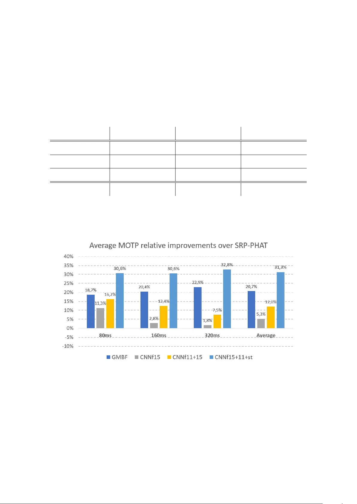
Article submitted for peer review to Sensors Journal on 2018/07/29 T owards End-to-End Acoustic Localization using Deep Learning: from Audio Signal to Source Position Coordinates Juan Manuel V era-Diaz, Daniel Pizarro ID and Javier Macias-Guarasa ID ∗ Department of Electronics, University of Alcalá, Campus Universitario s/n, 28805, Alcalá de Henar es, Madrid, Spain. manuel.vera@edu.uah.es, daniel.pizarro@uah.es, javier .maciasguarasa@uah.es * Correspondence: javier .maciasguarasa@uah.es; T el.: +34-91-885-6918 Academic Editor: name Received: date; Accepted: date; Published: date Abstract: This paper presents a novel appr oach for indoor acoustic source localization using microphone arrays and based on a Convolutional Neural Network (CNN). The pr oposed solution is, to the best of our knowledge, the first published work in which the CNN is designed to dir ectly estimate the three dimensional position of an acoustic source, using the raw audio signal as the input information avoiding the use of hand crafted audio features. Given the limited amount of available localization data, we propose in this paper a training strategy based on two steps. W e first train our network using semi-synthetic data, generated from close talk speech r ecordings, and wher e we simulate the time delays and distortion suffered in the signal that propagates from the source to the array of microphones. W e then fine tune this network using a small amount of real data. Our experimental results show that this strategy is able to produce networks that significantly impr ove existing localization methods based on SRP-PHA T strategies. In addition, our experiments show that our CNN method exhibits better resistance against varying gender of the speaker and differ ent window sizes compared with the other methods. Keywords: acoustic source localization; microphone arrays; deep learning; convolutional neural networks 1. Introduction The development and scientific research in advanced perceptual systems has notably grown during the last decades, and has experimented a tremendous rise in the last years due to the availability of increasingly sophisticated sensors, the use of computing nodes with higher and higher computational power , and the advent of powerful algorithmic strategies based on deep learning (all of them actually entering the mass consumer market). The aim of perceptual systems is to automatically analyze complex and rich information taken fr om differ ent sensors, in order to obtain refined information on the sensed envir onment and the activities being carried out within them. The scientific works in these environments, cover r esearch ar eas fr om basic sensor technologies, to signal processing and pattern recognition, and open the path to the idea of systems able to analyze human activities, providing them with advanced interaction capabilities and services.. In this context, localization of humans (being the most interesting element for perceptual systems) is a fundamental task that needs to be addr essed so that the systems can actually start to pr ovide higher level information on the activities being carried out. W ithout a precise localization, further advanced interaction between humans and their physical environment cannot be carried out successfully . The scientific community has devoted a huge amount of effort to build robust and reliable indoor localization systems, based on differ ent sensors [ 1 – 3 ]. Non-invasive technologies are preferr ed in this Sensors 2018 , xx , 1; doi:10.3390/sxx010001 www .mdpi.com/journal/sensors Sensors 2018 , xx , 1 2 of 18 context, so that no electronic or passive devices need to be carried by humans for localization. The two non-invasive technologies that have been mainly used in indoor localization are those based on video systems and acoustic sensors. This paper focuses on audio-based localization, with no previous assumptions on the acoustic signal characteristics nor in the physical environment, apart from the fact that unknown wide-band audio sources (e.g. human voice) are captur ed by a set of microphone arrays placed in known positions. The main objective of the paper is to directly use the signals captured by the microphone arrays to automatically obtain the position of the the acoustic source detected in the given envir onment. Even though ther e are a lot of proposals in this ar ea, Acoustic Source Localization (ASL) is still a hot resear ch topic. This paper proposes a convolutional neural network (CNN) architectur e that is trained end-to-end to solve the acoustic localization problem. T o our knowledge, this is the first work in the literatur e that does not pr ovide the network with featur e vectors extracted fr om the speech signals, but dir ectly uses the speech signal. A voiding hand crafted featur es has been pr oved to incr ease the accuracy of classification and regression methods based on convolutional neural networks in other fields, such as in computer vision [4,5]. Our proposal is evaluated using both semi-synthetic and real data, outperforming traditional solutions based on Steered Response Power ( SRP ) [ 6 ], that are still the basis of state-of-the-art systems [7 – 10]. The rest of the paper is organized as follows. In Section 2 a review study of the state-of-the-art in acoustic source localization with special emphasis on the use of deep learning appr oaches. Section 3 describes the CNN based proposal, with details on the training and fine tuning strategies. The experimental work is detailed in Section 4, and Section 5 summarizes the main conclusions and contributions of the paper and gives some ideas for future work. 2. State of the Art Many approaches exist in the literature to address the acoustic source localization (ASL) pr oblem. According to the classical literature review in this topic, these appr oaches can be br oadly divided in three categories [ 11 , 12 ]: time delay based, beamforming based, and high-resolution spectral-estimation based methods. This taxonomy relies in the fact that ASL has been traditionally considered a signal processing pr oblem based on the definition of a signal propagation model [ 11 – 19 ], but, more r ecently , the range of proposals in the literature also considered strategies based on exploiting optimization techniques and mathematical properties of related measurements [ 20 – 24 ], and also using machine learning strategies [ 25 – 27 ], aimed at obtaining a direct mapping from specific features to source locations [ 28 ], area in which deep learning approaches are starting to be applied and that will be further described later in this section. T ime delay based methods (also r eferred to as indirect methods ), compute the time dif ference of arrivals (TDOAs) across various combinations of pairs of spatially separated microphones, usually using the Generalized Corr elation Function (GCC) [ 13 ]. In a second step, the TDOAs ar e combined with knowledge of the microphones’ positions to generate a position estimation [11,29]. Beamforming based techniques [ 12 , 15 , 19 , 30 ] attempt to estimate the position of the source, optimizing a spatial statistic associated with each position, such as in the Steered Response Power ( SRP ) approach, in which the statistic is based on the signal power received when the microphone array is steered in the direction of a specific location. SRP-PHA T is a widely used algorithm for speaker localization based on beamforming that was first proposed in [ 6 ] 1 . It combines the robustness of the SRP approach with the Phase T ransform (PHA T) filtering, which increases the robustness of the algorithm to signal and room conditions, making it an ideal strategy for realistic speaker localization systems [ 16 , 17 , 32 – 34 ]. Other beamforming based methods such as the Minimum V ariance 1 Although the formulation is virtually identical to the Global Coherence Field (GCF) described in [31] Sensors 2018 , xx , 1 3 of 18 Distortionless Response (MVDR) [ 18 ], exhibits problems when facing reverberant environments, because it introduces a new trade-of f between dereverberation and noise r eduction. In what respect to spectral estimation based methods, the multiple signal classification algorithm (MUSIC) [ 35 ], has been widely used, but these methods, in general, tend to be less robust than beamforming methods [ 12 ], as they assume incoher ent signals and ar e very sensitive to small modeling errors. In the past few years, deep learning approaches [ 36 ] have taken the lead in differ ent signal processing and machine l earning fields, such as computer vision [ 37 , 38 ] and speech r ecognition [ 39 – 41 ], and, in general, in any area in which complex relationships between observed signals and the underlying processes generating them need to be discover ed. The idea of using neural networks for ASL is not new . Back in the early nineties and the first decade of the current century , works such as [ 25 , 42 , 43 ] proposed the use of neural network techniques in this area. However an evaluation on realistic and extensive data sets was not viable at this time, and the proposals wer e somehow limited in scope. W ith the advent and huge incr ease on applications of deep neural networks in all areas of machine learning, and mainly due to the sophisticated capabilities and more careful implementation details of network architectur es and the availability of advanced hardwar e architectur es with incr eased computational capacity , promising works have been pr oposed also for ASL [44 – 58]. The main differ ences between the different pr oposals using neural networks for ASL reside in the architectur es, input featur es, the network output (tar get), and the experimental setup (using r eal or simulated data). Regarding the information given to the neural network, we can find several works using features physically related to the ASL problem. Some of the proposals use features derived from the GCC or related functions, which actually make sense as these correlation function is closely related to the TDOAs which are used in traditional methods to generate position estimations. The published works use either the GCC coefficients directly [ 50 ], features derived from them [ 45 , 55 ] or from the correlation matrix [ 47 , 49 ], or even combined with others, such as cepstral coef ficients [ 53 ]. Other works are focused in exploiting binaural cues [ 44 , 46 ], features derived from convolving the spectrum with head related impulse responses [ 58 ] or even narr owband SRP values [ 56 ]. The latter approach goes one step further from corr elation related values, as the SRP function actually integrates multiple GCC estimations in such a way that acoustic energy maps can be easily generated fr om it. Opposed to the previously described works using refined featur es directly related to the localization problem, we can also find others using frequency domain features directly [ 48 , 52 ], in some cases generated from spectrograms of general time-frequency representations [ 51 , 54 ]. These approaches r epresent a step forwar d compar ed with the previous ones, as they give the network the responsibility of automatically learn the r elationship between spectral cues and the location related information [ 57 ] kind of combines both strategies, as they use spectral features but calculating them in a cross-spectral fashion, that is, combining the values from all the available microphones in the so-called Cross Spectral Map (CSM). In none of the r eferenced works, the authors try to make use of the raw acoustic signal dir ectly , and we ar e interested in evaluating the capabilities of CNN ar chitectur es in directly exploiting this raw input information. In what r espect to the estimation tar get, most of the works ar e oriented towar ds estimating the Direction of Arrival (DOA) of the acoustic sources [ 45 , 50 , 51 , 55 , 56 ], or DOA related measurements such as azimuth angle [ 44 , 46 , 48 ], elevation angle [ 58 ], or position bearing+range [ 53 ]. Some of the proposals pose the pr oblem not as a direct estimation (r egression) but as a classification problem among a predefined set of possible position related values [ 47 – 49 , 52 , 54 ] (azimuth, positions in a pr edefined grid, etc.). W orks with a very differ ent target try to estimate a clean acoustic sour ce map [ 57 ] or learn time-frequency masks as a pr eprocessing stage prior to ASL [59]. Sensors 2018 , xx , 1 4 of 18 In none of the refer enced works the authors try to dir ectly estimate the coordinate values of the acoustic sources, and, again, we ar e inter ested in evaluating the capabilities of CNN architectur es to directly generate this output information. Finally , in what respect to the experimental setup, most works use simulated data either for training or for training and testing [ 44 – 52 , 54 – 59 ], usually by convolving clean (anechoic) speech with impulse responses (room, head related, or DOA related (azimuth, elevation)). Only some of them actually face real recor dings [ 44 , 45 , 53 , 55 , 56 ], which in our opinion is a must to be able to assess the actual impact of the proposals in r eal conditions. So, in this paper we describe, for the first time in the literature to the best of our knowledge, a CNN architectur e in which we directly exploit the raw acoustic signal to be provided to the neural network, with the objective of directly estimating the three dimensional position of an acoustic source in a given environment. This is the reason why we refer to this strategy as end-to-end, considering the full coverage of the ASL problem. The proposal has been tested on both semi-synthetic and r eal data from a publicly available database. 3. System Description 3.1. Problem Statement Our system obtains the position of an acoustic source from the audio signals recor ded by an array of M microphones. Given a refer ence coordinate origin, the source position is defined with the 3D coordinate vector s =  s x s y s z  > . The microphones positions ar e known and they are defined with coordinate vectors m i =  m i , x m i , y m i , z  > with i = 1, . . . , M . The audio signal captured fr om the i th microphone is denoted by x i ( t ) . This signal is discretized with a sampling frequency f s and is defined with x i [ n ] . W e assume for simplicity that x i [ n ] is of finite-length with N samples. This corresponds to a small window of audio with duration w s = N / f s , which is a design parameter in our system. W e denote as x i the vector containing all time samples of the signal: x i =  x i [ 0 ] . . . x i [ N − 1 ]  > . (1) The problem we seek to solve is to find the following r egression function f : s = f ( x 1 , . . . , x N , m 1 , . . . , m M ) , (2) that obtains the speaker position given the signals recor ded from the micr ophones. In classical simplified approaches, f is found by assuming that signals received from dif ferent microphones mainly dif fer by a delay that depends on the relative position of the source with r espect to the microphones. However , this assumption breaks in environments wher e the signal suffers fr om random noise and distortion, such as multi-path signals or microphone non-linear r esponse. Due to the aforementioned effects, and the random nature of the audio signal, the regr ession function of equation (2) cannot be estimated analytically . W e present in this paper a learning approach for directly obtaining f using Deep Learning. W e represent f using a Convolutional Neural Network (CNN) which is learned end-to-end from the microphone signals. In our system we assume that microphones positions ar e fixed. W e thus drop the requir ement of knowing the microphone’s position from equation (2) which will be implicitly learned by our network with the following regr ession problem: s = f ne t ( x 1 , . . . , x M ) , (3) where f ne t denotes the function that we represent using the CNN and whose topology is described next. Sensors 2018 , xx , 1 5 of 18 3.2. Network T opology The topology of our neural network is shown in figure 1. It is composed of five convolutional blocks of one dimension and two fully connected blocks. Following equation (3), the network inputs are the set of windowed signals from the microphones and the network output is the estimated position of the acoustic source. Figure 1. Used network topology T able (1) shows the size and amount of convolutional filters in the proposed network. W e use filters of size 7 (layers 1 and 2), size 5 (layers 3 and 4) and size 3 (layer 5). The number of filters is 96 in the first two convolutional layers and 128 in the rest. As seen in figure 1, some of the layers are equipped with MaxPooling filters with the same pool size as their corresponding convolutional filters. The last two layers are fully-connected layers, one hidden with 500 nodes and the output layer . All layer ’s activation functions ar e “ReLUs” with the exception of the output layer . During training we include dropout with pr obability 0.5 in the fully-connected layers to prevent overfitting. T able 1. Network convolutional layers summary Block Filters Kernel Convolutional block 1 96 7 Convolutional block 2 96 7 Convolutional block 3 128 5 Convolutional block 4 128 5 Convolutional block 5 128 3 3.3. T raining Strategy The amount of available real data that we have in our experimental setup (see Section 4) will be, in general, limited for training a CNN model. T o cope with this problem we propose a training strategy comprising two steps: Step 1. T raining the network with semi-synthetic data: W e use close-talk speech recor dings and a set of randomly generated sour ce positions to generate simulated versions of the signals captured by a set of micr ophones that share the same geometry with the envir onment used in real data. Additional considerations on the acoustic behavior of the target environment (specific noise types, noise levels, etc.) is also taken into account to generate the data. This dataset can virtually be made as big as requir ed to train the network. Step 2. Fine tuning the network with real data: W e train the network on a reduced subset of the database captured in the target physical environment using the weights obtained in Step 1 as initialization. Sensors 2018 , xx , 1 6 of 18 3.3.1. Semi-Synthetic Dataset Generation In this step we extract audio signals from any available close-talk (anechoic) corpus, and use them to generate semi-synthetic data. There are many available datasets suitable for this task (freely of commercially distributed). Our semi-synthetic dataset can thus be made as big as required for training the CNN. For this task, we randomly generate position vectors q =  q x q y q z  > of the acoustic source using a uniform distribution that covers the physical space (room) that will be used. The loss function we use to train the network is the mean squar ed error between the estimated position given by the network ( s i ) and the target position vector ( q i ). It follows the expression: L ( Θ ) = 1 N N ∑ i = 1 | q i − s i | 2 , (4) where Θ repr esents the weights of the network. Equation (4) is minimized in function of the unknown weights using iterative optimization based on the Stochastic Gradient Descent (SGD) algorithm [ 60 ]. W e finally obtain the target weights θ ∈ Θ once a termination criterion is met in the optimization. More details are given in Section 4 about the training algorithm. In order to realistically simulate the signals received in the microphones from a given source position we have to consider two main issues: • Signal propagation considerations: This is affected by the impulse response of the target r oom. Differ ent alternatives can be used to simulate this effect, such as convolving the anechoic signals with real room impulse responses such as in [ 47 ], that can be difficult to acquire for general positions in big envir onments; or using r oom response simulation methods such as the image method [61] used in [62] for this purpose. • Acoustic noise conditions of the room and recording process conditions: These can be due to additional equipment (computers, fans, air conditioning systems, etc.) present in the room, and to problems in the signal acquisition setup. This can be addressed by assuming additive noise conditions, and selecting a noise type and acoustic effects that should be preferably estimated in the target r oom. In our case, and regarding the first issue, we used an initial simple approach, just taking into account the propagation delay fr om the source position to each of the micr ophones, that depends on their relative position and the sound speed in the r oom. W e denote the number of samples we have to shift a signal to simulate the arrival d elay suf fered at microphone i by N s i = f s d i c where f s is the sampling frequency of the signal, d i is the euclidean distance between the acoustic source and the i microphone and c is the sound speed in air ( c = 343 m / s in a room at 20 C o ). In general N s i is not an integer number . W e thus requir e a way to simulate sub-sample shifts in the signal. In order to implement the delay N s i on x pc (the windowed signal of N samples from the close-talk dataset) to obtain x i we use the following transformation: X pc = F { x pc } x i = A i  F − 1 { X pc D s i  , wi t h D s i =  1, e − j 2 π N s i N , e − j 4 π N s i N , · · · , e − j ( N − 1 ) 2 π N s i N  (5) where we first transform x pc into the fr equency domain X pc using the Discr ete Fourier T ransform operator F . W e then change its phase accor ding to N s i by the phase vector D s i and transform the signal back into time domain x i , using the Inverse Discrete Fourier T ransform operator F -1 . A i is an amplitude factor applied to the signal that follows a uniform random distribution, and it is different for each microphone, pr eventing the network from being affected by amplitude dif ferences between the signals captured in dif ferent micr ophones ( A i ∈ [ 0.01, 0.03 ] in the experimental setup described in Section 4). Regarding the second issue, we simulate noise and disturbances in the signals arriving to the microphones so that the signal-to-noise ratio and the spectral content of the signals ar e as similar as Sensors 2018 , xx , 1 7 of 18 possible to those found in the real data. In order to provide an example of the methodology we follow , we refer in this section to the particular case of the IDIAP room (see Section 4.1.1) that will be used in our real data experiments, and the Albayzin Phonetic Corpus (see Section 4.1.2) that will be used for synthetic data generation. In the IDIAP room, a spectrogram based analysis showed that the recor dings ar e contaminated with a tone at around 25 H z in the spectrum which does not appear in anechoic conditions, pr obably due to room equipment of electrical noise generated in the recor ding hardwar e setup. W e have determined that the frequency of this tone actually varies in a range between 20 H z and 30 H z . So, in the synthetic data generation pr ocess, we have contaminated the signals fr om the phonetic corpus with an additive tone of a random frequency in this established range, and we have also added white gaussian noise following the expression: x pc ne w [ n ] = x pc [ n ] + k s sin ( 2 π f 0 n / f s + φ 0 ) + k η η w gn [ n ] , (6) where k s is a scaling factor for the contaminating tone signal (similar to the tone amplitude found in the target room recor dings, 0.1 in our case), f 0 ∈ [ 20, 30 ] H z , φ 0 ∈ [ 0, π ] r a d , η w gn is a white gaussian noise signal, and k η is a noise scaling factor to generate signals with a SNR which is similar to that found in the target r oom recor dings. After this procedur e is applied, the semi-synthetic signal data set will be ready to be used in the neural network training procedur e. 3.3.2. Fine T uning Procedur e The previous step takes car e of repr oducing simple acoustic characteristics of the testing room such as the propagation effects and the presence of specific types and levels of additive noises, but there ar e other phenomena like multi-path and reverberation pr opagation which are more complex to simulate. In order to introduce these acoustic behaviors of the target physical environment, our proposal is to carry out a fine tuning procedure of the network model using a short amount of real recor ded data in the target r oom Although there ar e other methods such as the one proposed in [ 49 ], where an unsupervised DNN is implemented for the adaptation of parameters to unknown data, we believe that the fine tuning process implemented is adequate because, in the first place, it is a supervised pr ocess with which a better performance is expected to be obtained and, secondly , not all the sequences of the test data set are used, so that only a few ar e used for the fine tuning process, saving the r est for the test phase. 4. Experimental W ork In his section we describe the datasets used in both steps of the training strategy described in Section 3.3, and the details associated with it. W e then define the experimental setup general conditions, and the error metrics used for comparing our proposal with other state-of-the-art methods and finally present our experimental r esults, starting from the baseline performance we aim at impr oving. 4.1. Datasets 4.1.1. IDIAP A V16.3 Corpus: for testing and fine tuning W e have evaluated our proposal using the audio recor dings of the A V16.3 database [ 63 ], an audio-visual corpus r ecorded in the Smart Meeting Room of the IDIAP r esearch institute, in Switzerland. W e have also used the physical layout of this room for our semi-synthetic data generation process. The IDIAP Smart Meeting Room is a 3.6 m × 8.2 m × 2.4 m rectangular r oom with a rectangular table centrally located and measuring 4.8 m × 1.2 m . On the table’s surface there are two circular micr ophone arrays of 0.1 m radius, each of them composed by 8 regularly distributed microphones as shown in figure 2. The centers of both arrays are separated by a distance of 0.8 m . The middle point between Sensors 2018 , xx , 1 8 of 18 them is considered as the origin of the coordinate refer ence system. A detailed description of the meeting room can be found in [64]. The dataset is composed by several sequences of recor dings, synchronously sampled at 16 KHz, which a wide range of experimental conditions in the number of speakers involved and their activity . Some of the available audio sequences are assigned a corresponding annotation file containing the real ground truth positions (3D coordinates) of the speaker ’s mouth at every time frame in which that speaker was talking. The segmentation of acoustic frames with speech activity was first checked manually at certain time instances by a human operator in order to ensure its correctness, and later extended to cover the rest of recording time by means of interpolation techniques. The frame shift r esolution was defined to be 40 ms. The complete dataset is fully accessible on-line at [65]. (a) (b) (c) Figure 2. (a) Simplified top view of the IDIAP Smart Meeting Room , (b) A real picture of the room extracted from a video frame, (c) Micr ophone setup used in this proposal In this paper we will just focus on all the annotated sequences of this dataset featuring a single speaker , whose main characteristics are shown in T able 2. This allows us to directly compare our performance with the state-of-the-art method presented in [ 20 ]. Note that the firsts three sequences are performed by a speaker remaining static while speaking at differ ent positions, and the last two ones by a moving speaker , being all of the speakers dif ferent. W e will refer to these sequences as s0 1, s0 2, s0 3, s1 1 and s1 5 for brevity . Sensors 2018 , xx , 1 9 of 18 T able 2. IDIAP Smart Meeting Room used sequences. Sequence A verage speaker height (cm) ∗ Duration (seconds) Number of ground truth frames Description seq01-1p-0000 54.3 208 2248 A single male speaker , static while speaking, at each of 16 locations. The speaker is facing the microphone arrays. seq02-1p-0000 62.5 171 2411 A single female speaker , static while speaking, at each of 16 locations. The speaker is facing the microphone arrays. seq03-1p-0000 70.3 220 2636 A single male speaker , static while speaking, at each of 16 locations. The speaker is facing the microphone arrays. seq11-1p-0100 53.5 33 481 A single male speaker , making random movements while speaking, and facing the arrays. seq15-1p-0100 79.5 36 436 A single male speaker , walking around while alternating speech and long silences. No constraints ∗ The average speaker height is refer enced to the system coordinates and refers to the speaker ’s mouth height. 4.1.2. Albayzin Phonetic Corpus: for Semi-Synthetic Dataset Generation The Albayzin Phonetic Corpus [ 66 ] consists of 3 sub-corpora of 16 kHz 16 bits signals, recor ded by 304 Castilian Spanish speakers in a professional recording studio using high quality close talk microphones. W e use this dataset to generate semi-synthetic data as described in Section 3.3.1. Fr om the 3 sub-corpora, we will be only using the so-called phonetic corpus [ 67 ], composed of 6800 utterances of phonetically balanced sentences. This phonetical balance characteristic makes this dataset perfect for generating our semi-synthetic data, as it will cover all possible acoustic contexts. 4.2. T raining and Fine T uning Details In the semi-synthetic dataset generation procedur e, described in Section 3.3.1, we generate random positions q with uniformly distributed values in the following intervals: q x ∈ [ 0, 3.6 ] m , q y ∈ [ 0, 8.2 ] m and q z ∈ [ 0.92, 1.53 ] m , which correspond to the possible distribution of the speaker ’s mouth positions in the IDIAP room [63]. Regarding the optimization strategy for the loss function described by equation (4) we employ the ADAM [ 68 ] optimizer (variant of SGD with variable learning rate) along 200 epochs with a batch size of 100 samples. 7200 different frames of input data per epoch ar e randomly generated during the training phase and other 800 for validation. The experiments will be performed with three dif ferent window lengths (80 ms , 160 ms and 320 ms ), so the training phase will be run once per window length, obtaining three dif fer ent network models. In each training, 200 audio r ecordings are randomly chosen and 40 dif ferent windows ar e randomly extracted from each. In the same way , 200 acoustic sour ce position q vectors are randomly generated so that each position generates 40 windows of the same signal. For the fine tuning procedur e described in Section 3.3.2, we will be mainly using sequences s1 1 and s1 5, that features a speaker moving in the room while speaking, and also sequences s0 1, s0 2 and s0 3 in a final experiment. As it will be described in Section 4.6, we will also address experiments trying to assess the relevance of adding additional sequences s0 1, s0 2 and s0 3 to complement the fine tuning data provided by s1 1 and s1 5. W e will also refer to gender and height issues in the fine tuning and evaluation data. Sensors 2018 , xx , 1 10 of 18 4.3. Experimental Setup In our experiments, sequences s0 1, s0 2 and s0 3 are used for testing the performance of our network and, as explained above, to complement sequences s1 1 and s1 5 for fine tuning. In this work, we are using a simple microphone array configuration, aimed at evaluating our proposal in a r esour ce-restricted envir onment, as it was done in [ 20 ]. In order to do so, we ar e using 4 microphones (numbers 1, 5, 11 and 15, out of the 16 available in the A V16.3 data set), gr ouped in two microphone pairs. The selected microphone pairs configurations are shown in Figure 2.c, in which microphones with the same color are consider ed as belonging to the same microphone pair . W e provide r esults depending on the length of the acoustic frame, for 80 ms , 160 ms and 320 ms , to precisely assess to what extent the improvements ar e consistent with varying acoustic time resolutions. The main interest of our experimental work is assessing whether the end-to-end CNN based approach (that we will r efer to as CNN) is competitive as compared with state-of-the-art localization methods. W e will compare this CNN appr oach with the standard SRP-PHA T method, and the recent strategy proposed in [ 20 ] that we will refer to as GMBF . This GMBF method is based on fitting a generative model to the GCC-PHA T signals using sparse constraints, and it reported significant improvements over SRP-PHA T in the IDIAP dataset [20,69]. After providing baseline results comparing SRP-PHA T , GMBF and our proposal without fine tuning procedur e, we will then describe four experiments, that we briefly summarize here: • In the first experiment, we will evaluate the performance improvements when using a single sequence for the fine tuning procedur e. • In the second experiment, we will evaluate the dif ferences between the semi-synthetic training plus the fine tuning approach, versus just training the network fr om scratch. • In the third experiment, we will evaluate the impact of adding an additional fine tuning sequence. • In the last experiment, we will evaluate the final performance improvements when also adding static sequences to the refinement pr ocess. 4.4. Evaluation metrics Our CNN based approach yields a set of spatial coordinates s k =  s k , x s k , y s k , z  > that are estimations of the current speaker position as time instant k . These position estimates will be compar ed, by means of the Euclidean distance, to the ones labeled in a transcription file containing the real positions s k G T ( ground truth ), of the speaker . W e evaluate performance adopting the same metric used in [ 20 ] and developed under the CHIL project [70]. It is known as MOTP ( Multiple Object T racking Precision ) and is defined as: MO T P = N P ∑ k = 1 | s k G T − s k | 2 N P , (7) where N P denotes the total number of position estimations along time, s k the estimated position vector and s k G T the labeled ground tr uth position vector . W e will compare our experimental results, and that of the GMBF method, with that of SRP-PHA T , measuring the relative impr ovement in MOTP with method, that is defined as follows: ∆ MO T P r = 100 MO T P S R P − P H AT − MO T P pro p o sa l MO T P S R P − P H AT [ % ] (8) 4.5. Baseline Results The baseline r esults are shown in T able 3 for sequences s0 1, s0 2 and s0 3, and all the evaluated time window sizes (in all the tables showing results in this paper , bold font highlight the best ones for a given data sequence and window length). The T able shows the results achieved by the SRP-PHA T Sensors 2018 , xx , 1 11 of 18 standard algorithm strategy (columns SRP), the alternative described in [ 20 ] (columns GMBF), and the proposal in this paper without applying the fine-tuning procedure (columns CNN). W e also show the relative impr ovements of GMBF and CNN as compared with SRP-PHA T . T able 3. Baseline results for the SRP-PHA T strategy (columns SRP); the one in [ 20 ] (columns GMBF), and the CNN trained with synthetic data without applying the fine-tuning pr ocedure (columns CNN) for sequences s0 1, s0 2 and s0 3 for different window sizes. Relative improvements as compared to SRP-PHA T are shown below the MOTP values. 80 m s 160 m s 320 m s SRP GMBF CNN SRP GMBF CNN SRP GMBF CNN s0 1 MO T P ( m ) ∆ MO T P r 1.020 0 . 7 9 5 1.615 0.910 0.686 1.526 0.830 0 . 5 8 8 1.464 22 . 1 % − 58.3% 24 . 6 % − 67.7% 29 . 1 % − 76.4% s0 2 MO T P ( m ) ∆ MO T P r 0.960 0 . 8 6 4 2.124 0.840 0 . 7 5 9 1.508 0.770 0 . 6 94 1.318 10 . 0 % − 121.3% 9 . 6 % − 79.5% 9 . 9 % − 71.2% s0 3 MO T P ( m ) ∆ MO T P r 0.900 0 . 6 8 6 1.559 0.770 0 . 5 6 3 1.419 0.690 0 . 4 84 1.379 23 . 8 % − 73.2% 26 . 9 % − 84.3% 29 . 9 % − 99.9% A verage MO T P ( m ) ∆ MO T P r 0.957 0 . 7 7 8 1.763 0.836 0 . 6 6 6 1.481 0.760 0 . 5 85 1.385 18 . 7 % − 84.3% 20 . 4 % − 77.1% 22 . 9 % − 82.3% The main conclusions from the baseline r esults are: • Best MOTP values for the standard SRP-PHA T algorithm are around 69 cm , with averages between 76 cm and 96 cm . For the GMBF , best MOTP values are around 48 cm , with averages between 59 c m and 78 cm . • MOTP values improve as the frame size increases, as expected, given that better correlation values will be estimated for longer window signal lengths. • The GMBF strategy , as described in [ 20 ], achieves very relevant impr ovements as compared with SRP-PHA T , with average relative improvements ar ound 20%, and peak values of almost 30%. • Our CNN strategy , which at this point is only trained with semi-synthetic data, is very far from reaching the SRP-PHA T or GMBF in terms of performance. This r esult leads us to think that there are other ef fects only present in r eal data, such as reverberation, that ar e af fecting the network. Given the discussion above, we decided to apply the fine tuning strategy discussed in Section 3.3.2, with the experimental details described in Section 4.2. So, the results shown in T able 3 will be compar ed with those obtained by our CNN method, under dif ferent fine tuning (and training) conditions, and will be described below . 4.6. Results and Discussion The first experiment in which we applied the fine tuning pr ocedur e used s1 5 as the fine tuning subset. T able 4 shows the results obtained by GMBF (columns GMBF) and CNN with this fine tuning strategy (columns CNNf15 ). From the table results it can be seen that CNNf15 is, most of the times, better than the SRP-PHA T baseline (except in two cases for s0 3 in which there was a slight degradation). The average performance shows a consistent improvement of CNNf15 compared with SRP-PHA T , between 1.8% and 11.3%. However CNNf15 is still behind GMBF in all cases but one (for s0 2 and 80 m s ). Sensors 2018 , xx , 1 12 of 18 T able 4. Results for the stratgy in [ 20 ] (columns GMBF); and the CNN fine tuned with sequence s1 5 (columns CNNf15). 80 m s 160 m s 320 m s GMBF CNNf15 GMBF CNNf15 GMBF CNNf15 s0 1 MO T P ( m ) ∆ MO T P r 0 . 7 9 5 0.875 0 . 6 86 0.833 0 . 5 88 0.777 22 . 1 % 14.2% 2 4 . 6 % 8.5% 29 . 1 % 6.4% s0 2 MO T P ( m ) ∆ MO T P r 0.864 0 . 8 3 9 0 . 75 9 0.801 0 . 6 9 4 0.731 10.0% 1 2 . 6 % 9 . 6 % 4.6% 9 . 9 % 5.1% s0 3 MO T P ( m ) ∆ MO T P r 0 . 6 8 6 0.835 0 . 5 63 0.806 0 . 4 84 0.734 23 . 8 % 7.2% 26 . 9 % -4.7% 29 . 9 % -6.4% A verage MO T P ( m ) ∆ MO T P r 0 . 7 7 8 0.849 0 . 6 66 0.813 0 . 5 85 0.746 18 . 7 % 11.3% 2 0 . 4 % 2.8% 2 2 . 9 % 1.8% Our conclusion is that the fine tuning procedure is able to effectively complement the trained models from synthetic data, leading to results that outperform SRP-PHA T . This is specially relevant as: • The amount of fine tuning data is limited (only 36 seconds, corresponding to 436 frames, as shown in T able 2), thus opening the path to further improvements with a limited data recording effort. • The speaker used for fine tuning was mostly moving while speaking, while in the testing sequences the speakers are static while speaking. This means that the fine tuning material include far more active positions than in the testing sequences, and the network is able to extract the relevant information for the tested positions. • The speaker used for fine tuning is a male, and the obtained results for male speakers (sequences s0 1 and s0 3) and the female one (sequence s0 2) do not seem to show any gender-dependent bias, which means that the gender issue does not seem to play a role in the adequate adaptation of the network models. When comparing the results of T able 3 and T able 4, and given the large improvement when applying the fine tuning strategy , we could think that the effect of the initial training with semi-synthetic data is limited. From this argument, we r un an additional training experiment in which we just trained the network from scratch using s1 5, aiming at assessing the actual effect of semi-synthetic training+fine tuning versus just training with real r oom data. T able 5 shows the comparison between these two options: training from scratch using s1 5 (columns CNNt15) and semi-synthetic training+fine tuning with s1 5 (columns CNNf15). The average improvement of the latter approach varies between 1.8% and 11.3% with an average improvement over all window lengths of 5.3%, while the training from scratch average improvement varies between − 20.6% and 4.3% with an average value of − 7.0%. These differences show that the training+fine tuning proposal outperforms training the network fr om scratch, thus validating our methodology . T able 5. Results for the CNN proposal, either trained from scratch with sequence s1 5 (columns CNNt15) or fine tuned with sequence s1 5 (columns CNNf15). 80 m s 160 m s 320 m s CNNt15 CNNf15 CNNt15 CNNf15 CNNt15 CNNf15 s0 1 MO T P ( m ) ∆ MO T P r 1.009 0 . 8 7 5 0.949 0 . 8 33 1.0009 0 . 7 77 1.1% 14 . 2 % − 4.3% 8 . 5 % − 21.6% 6 . 4 % s0 2 MO T P ( m ) ∆ MO T P r 0 . 8 0 7 0.839 0 . 7 67 0.801 0.807 0 . 7 3 1 15 . 9 % 12.6% 8 . 7 % 4.6% − 4.8% 5 . 1 % s0 3 MO T P ( m ) ∆ MO T P r 0.935 0 . 8 3 5 0.911 0 . 8 06 0.936 0 . 7 34 − 3.9% 7 . 2 % − 18.3% − 4 . 7 % − 35.7% − 6 . 4 % A verage MO T P ( m ) ∆ MO T P r 0.915 0 . 8 4 9 0.875 0 . 8 13 0.916 0 . 7 46 4.3% 11 . 3 % − 4.6% 2 . 8 % − 20.6% 1 . 8 % Sensors 2018 , xx , 1 13 of 18 In spite of the r elevant improvements with the fine tuning appr oach, they are still far fr om making this suitable for further competitive exploitation in the ASL scenario (provided we have the GMBF alternative), so that we next aim at increasing the amount of fine tuning material. In our third experiment, we applied the fine tuning procedure using an additional moving speaker sequence, that is, including s1 5 and s1 1 in the fine tuning subset. T able 6 shows the results obtained by GMBF and CNN fine tuned with s1 5 and s1 1 (CNNf15+11 columns). In this case, we see additional improvements over using only s1 5 for fine tuning, and there is only one case in which CNNf15+11 does not outperforms SRP-PHA T (with a marginal degradation of − 0.3%). T able 6. Relative improvements over SRP-PHA T for the strategy in [ 20 ] (columns GMBF); and the CNN fine tuned with sequences s1 5 and s1 1 (columns CNNf15+11) 80 m s 160 m s 320 m s GMBF CNNf15+11 GMBF CNNf15+11 GMBF CNNf15+11 s0 1 MO T P ( m ) ∆ MO T P r 0 . 7 9 5 0.805 0 . 68 6 0.750 0 . 58 8 0.706 22 . 1 % 21.1% 2 4 . 6 % 17.6% 29 . 1 % 14.9% s0 2 MO T P ( m ) ∆ MO T P r 0.864 0 . 80 9 0.759 0 . 71 6 0 . 6 94 0.712 10.0% 15 . 7 % 9.6% 14 . 8 % 9.9% 7.5% s0 3 MO T P ( m ) ∆ MO T P r 0 . 6 8 6 0.792 0 . 56 3 0.732 0 . 48 4 0.692 23 . 8 % 12.0% 2 6 . 9 % 4.9% 2 9 . 9 % − 0.3% A verage MO T P ( m ) ∆ MO T P r 0 . 7 7 8 0.802 0 . 66 6 0.732 0 . 58 5 0.703 18 . 7 % 16.2% 2 0 . 4 % 12.4% 22 . 9 % 7.5% The CNN based approach shows again an average consistent improvement compared with SRP-PHA T between 7.5% and 16.2%. In this case, the newly added sequence ( s1 1, with a duration of only 33 seconds) for fine tuning corresponds to a randomly moving male speaker , and the results show that its addition contributes to further improvements in the CNN based proposal, but it is still behind GMBF in all cases but two, but with results getting closer . This suggests that a further increment in the fine tuning material should be considered. Our last experiment will consist of fine tuning the network including also additional static speaker sequences. T o assur e that the training (including fine tuning) and testing material are fully independent, we will fine tune with s1 5, s1 1 and with the static sequences that are not tested in each experiment run, as shown in T able 7. T able 7. Fine tuning material used in the experiment corresponding to T able 8 columns CNNf15+11+st. T est sequence Fine tuning sequences seq01 s1 5 + s1 1 + s0 2 + s0 3 seq02 s1 5 + s1 1 + s0 1 + s0 3 seq03 s1 5 + s1 1 + s0 1 + s0 2 T able 8 shows the results obtained for this fine tuning scenario, and the main conclusions are: • The CNN based method exhibits much better average behavior than GMBF for all window sizes. A verage absolute improvement against SRP-PHA T for the CNN is more than 10 points higher than for GMBF , reaching 31.3% in the CNN case and 20.7% for GMBF . • Considering individual sequences, CNN is significantly better than GMBF for sequences s0 1 and s0 2, and slightly worse for s0 3. • Considering the best individual result, maximum improvement for the CNN is 41.6% ( s0 1, 320 m s ), while the top result for GMBF is 29.9% ( s0 3, 320 m s ). • The effect of adding static sequences is beneficial, as expected, provided that the acoustic tuning examples will be generated fr om positions which are similar , but not identical, as the speakers Sensors 2018 , xx , 1 14 of 18 have varying heights and their position in the room is not strictly equal from sequence to sequence. • The improvements obtained are significant and come at the cost of additional fine tuning sequences. However , this extra cost is still reasonable, as the extra fine tuning material is of limited duration, around 400 seconds in average (6.65 minutes). T able 8. Relative improvements over SRP-PHA T for the strategy in [ 20 ] (columns GMBF); and the CNN fine tuned with the sequences described in T able 7 (columns CNNf15+11+st) 80 m s 160 m s 320 m s GMBF CNNf15+11+st GMBF CNNf15+11+st GMBF CNNf15+11+st s0 1 MO T P ( m ) ∆ MO T P r 0.795 0 . 6 0 7 0.686 0 . 5 40 0.588 0 . 4 85 22.1% 40 . 5 % 24.6% 4 0 . 7 % 29.1% 41 . 6 % s0 2 MO T P ( m ) ∆ MO T P r 0.864 0 . 6 6 9 0.759 0 . 5 79 0.694 0 . 5 45 10.0% 30 . 3 % 9.6% 31 . 1 % 9.9% 29 . 2 % s0 3 MO T P ( m ) ∆ MO T P r 0 . 6 8 6 0.707 0 . 5 63 0.617 0 . 4 84 0.501 23 . 8 % 21.4% 2 6 . 9 % 19.9% 29 . 9 % 27.4% A verage MO T P ( m ) ∆ MO T P r 0.778 0 . 6 6 4 0.666 0 . 5 81 0.585 0 . 5 11 18.7% 30 . 6 % 20.4% 3 0 . 6 % 22.9% 32 . 8 % Finally , to summarize, Figure 3 shows the average MOTP relative improvements over SRP-PHA T obtained by our CNN proposal using differ ent fine tuning subsets, and its comparison with the GMBF results, for all the signal window sizes. Figure 3. MOTP relative improvements over SRP-PHA T for GMBF and CNN using differ ent fine tuning subsets (for all window sizes). From the results obtained by our proposal, it is clear that the highest contribution to the improvements fr om the bar e CNN training is the fine tuning procedure with limited data (CNNf15, comparing T ables 3 and 4), while the addition of additional fine tuning material consistently improves the results (T ables 6, and 8). It is again worth noticing that these improvements are consistently independent of the gender of the considered speaker and whether there is a match or not between the static or dynamic activity of the speakers being used in the fine tuning subsets. This suggest that the network is actually learning the acoustic cues that ar e related to the localization pr oblem, so that we can conclude that our proposal is a suitable and pr omising strategy for solving the ASL task. Sensors 2018 , xx , 1 15 of 18 5. Conclusions W e have presented in this paper the first audio localization CNN that is trained end-to-end from the audio signals to the source position. W e show that this method is very promising, outperforming the state-of-the-art methods [ 20 , 69 ] and those using SRP-PHA T , given that suf ficient fine tuning data is available. In addition, our experiments show that the CNN method exhibits good r esistance against varying gender of the speaker and dif ferent window sizes compared with the baseline methods. Given that the amount of data recor dings for audio localization is limited at the moment, we have thus proposed in the paper to first train the network using semi-synthetic data followed by fine tuning using a small amount of real data. This has been a common strategy in other fields to prevent overfitting, and we show in the paper that it significantly improves the system performance as compared with training the network from scratch using r eal data. In a future line of work we plan to improve the generation of semi-synthetic data including reverberation effects and testing in detail the effects of gender and language in the system performance. In addition we plan to include more real data by developing a large corpus for audio localization, that will be made available to the scientific community for resear ch purposes. Also, an extensive evaluation will be carried out to asses the impact of the proposal with more complex acquisition scenarios (comprising a higher number of microphone pairs). Author Contributions: Conceptualization, Daniel Pizarro; Methodology , W riting - review & editing and visualization, Daniel Pizarr o, Juan Manuel V era-Diaz and Javier Macias-Guarasa; Investigation, Juan Manuel V era-Diaz; W riting - original draft, Juan Manuel V era-Diaz; Software, Daniel Pizarro and Juan Manuel V era-Diaz; Resources Javier Macias-Guarasa; Funding Acquisition, Daniel Pizarr o and Javier Macias-Guarasa Funding: Parts of this work were funded by the Spanish Ministry of Economy and Competitiveness under projects HEIMDAL (TIN2016-75982-C2-1-R), AR TEMISA (TIN2016-80939-R), and SP ACES-UAH (TIN2013-47630-C2-1-R), and by the University of Alcalá under projects CCGP2017/EXP-025 and CCG2016/EXP-010. Juan Manuel V era-Diaz is funded by Comunidad de Madrid and FEDER under contract reference number PEJD-2017-PRE/TIC-4626. Conflicts of Interest: The authors declare no conflict of interest. 1. T orres-Solis, J.; Falk, T .H.; Chau, T . A r eview of indoor localization technologies: towards navigational assistance for topographical disorientation. In Ambient Intelligence ; InT ech, 2010. 2. Ruiz-López, T .; Garrido, J.L.; Benghazi, K.; Chung, L. A survey on indoor positioning systems: foreseeing a quality design. In Distributed Computing and Artificial Intelligence ; Springer , 2010; pp. 373–380. 3. Mainetti, L.; Patrono, L.; Ser gi, I. A survey on indoor positioning systems. Software, T elecommunications and Computer Networks (SoftCOM), 2014 22nd International Conference on. IEEE, 2014, pp. 111–120. 4. Krizhevsky , A.; Sutskever , I.; Hinton, G.E. Imagenet classification with deep convolutional neural networks. Advances in neural information processing systems, 2012, pp. 1097–1105. 5. Simonyan, K.; Zisserman, A. V ery deep convolutional networks for large-scale image r ecognition. arXiv preprint arXiv:1409.1556 2014 . 6. DiBiase, J. A high-accuracy , low-latency technique for talker localization in reverberant environments using microphone arrays. PhD thesis, Brown University , 2000. 7. Nunes, L.O.; Martins, W .A.; Lima, M.V .; Biscainho, L.W .; Costa, M.V .; Goncalves, F .M.; Said, A.; Lee, B. A steered-r esponse power algorithm employing hierar chical search for acoustic source localization using microphone arrays. IEEE T ransactions on Signal Processing 2014 , 62 , 5171–5183. 8. Cobos, M.; García-Pineda, M.; Arevalillo-Herráez, M. Steered response power localization of acoustic passband signals. IEEE Signal Processing Letters 2017 , 24 , 717–721. 9. He, H.; W ang, X.; Zhou, Y .; Y ang, T . A steered r esponse power approach with trade-of f prewhitening for acoustic source localization. The Journal of the Acoustical Society of America 2018 , 143 , 1003–1007. 10. Salvati, D.; Drioli, C.; Foresti, G.L. Sensitivity-Based Region Selection in the Steered Response Power Algorithm. Signal Processing 2018 . Sensors 2018 , xx , 1 16 of 18 11. Brandstein, M.S.; Silverman, H.F . A practical methodology for speech source localization with microphone arrays. Computer Speech & Language 1997 , 11 , 91–126. doi:10.1006/csla.1996.0024. 12. DiBiase, J.; Silverman, H.; Brandstein, M. Robust localization in reverberant rooms. Microphone Arrays 2001 , pp. 157–180. 13. Knapp, C.; Carter , G. The generalized correlation method for estimation of time delay . Acoustics, Speech and Signal Processing, IEEE T ransactions on 1976 , 24 , 320 – 327. doi:10.1109/T ASSP .1976.1162830. 14. Zhang, C.; Florencio, D.; Zhang, Z. Why does PHA T work well in low noise, reverberative envir onments? Acoustics, Speech and Signal Processing, 2008. ICASSP 2008. IEEE International Conference on, 2008, pp. 2565 –2568. doi:10.1109/ICASSP .2008.4518172. 15. Dmochowski, J.P .; Benesty , J. Steered Beamforming Approaches for Acoustic Sour ce Localization. In Speech Processing in Modern Communication ; Cohen, I.; Benesty , J.; Gannot, S., Eds.; Springer Berlin Heidelberg, 2010; V ol. 3, Springer T opics in Signal Processing , pp. 307–337. 10.1007/978-3-642-11130-3_12. 16. Cobos, M.; Marti, A.; Lopez, J. A modified SRP-PHA T functional for robust real-time sound source localization with scalable spatial sampling. Signal Processing Letters, IEEE 2011 , 18 , 71–74. 17. Butko, T .; Gonzalez Pla, F .; Segura Perales, C.; Nadeu Camprubí, C.; Hernando Pericás, F .J. T wo-source acoustic event detection and localization: online implementation in a smart-r oom. Proceedings of the 17th European Signal Pr ocessing Conference (EUSIPCO’11), 2011, pp. 1317–1321. 18. Habets, E.A.P .; Benesty , J.; Gannot, S.; Cohen, I. The MVDR Beamformer for Speech Enhancement. In Speech Processing in Modern Communication ; Cohen, I.; Benesty , J.; Gannot, S., Eds.; Springer Berlin Heidelberg, 2010; V ol. 3, Springer T opics in Signal Processing , pp. 225–254. 10.1007/978-3-642-11130-3_9. 19. Marti, A.; Cobos, M.; Lopez, J.J.; Escolano, J. A steered response power iterative method for high-accuracy acoustic source localization. The Journal of the Acoustical Society of America 2013 , 134 , 2627–2630, [https://doi.org/10.1121/1.4820885]. doi:10.1121/1.4820885. 20. V elasco, J.; Pizarro, D.; Macias-Guarasa, J. Sour ce Localization with Acoustic Sensor Arrays Using Generative Model Based Fitting with Sparse Constraints. Sensors 2012 , 12 , 13781–13812. doi:10.3390/s121013781. 21. Padois, T .; Sgar d, F .; Doutres, O.; Berry , A. Comparison of acoustic source localization methods in time domain using sparsity constraints. 2015. cited By 0. 22. V elasco, J.; Pizarro, D.; Macias-Guarasa, J.; Asaei, A. TDOA Matrices: Algebraic Properties and Their Application to Robust Denoising W ith Missing Data. IEEE T ransactions on Signal Processing 2016 , 64 , 5242–5254. doi:10.1109/TSP .2016.2593690. 23. Compagnoni, M.; Pini, A.; Canclini, A.; Bestagini, P .; Antonacci, F .; T ubaro, S.; Sarti, A. A Geometrical-Statistical Approach to Outlier Removal for TDOA Measur ements. IEEE T ransactions on Signal Processing 2017 , 65 , 3960–3975. doi:10.1109/TSP .2017.2701311. 24. Salari, S.; Chan, F .; Chan, Y .T .; Read, W . TDOA Estimation W ith Compressive Sensing Measurements and Hadamard Matrix. IEEE T ransactions on Aerospace and Electronic Systems 2018 , pp. 1–1. doi:10.1109/T AES.2018.2826230. 25. Murray , J.C.; Erwin, H.R.; W ermter , S. Robotic sound-sour ce localisation ar chitecture using cr oss-correlation and recurr ent neural networks. Neural Networks 2009 , 22 , 173 – 189. What it Means to Communicate, doi:https://doi.org/10.1016/j.neunet.2009.01.013. 26. Deleforge, A. Acoustic Space Mapping: A Machine Learning Approach to Sound Source Separation and Localization. Theses, Université de Grenoble, 2013. 27. Salvati, D.; Drioli, C.; Foresti, G.L. On the use of machine learning in microphone array beamforming for far-field sound sour ce localization. 2016 IEEE 26th International W orkshop on Machine Learning for Signal Processing (MLSP), 2016, pp. 1–6. doi:10.1109/MLSP .2016.7738899. 28. Rascon, C.; Meza, I. Localization of sound sources in robotics: A review . Robotics and Autonomous Systems 2017 , 96 , 184 – 210. doi:https://doi.org/10.1016/j.robot.2017.07.011. 29. Stoica, P .; Li, J. Lecture Notes - Source Localization from Range-Differ ence Measurements. IEEE Signal Processing Magazine 2006 , 23 , 63–66. doi:10.1109/SP-M.2006.248717. 30. Cobos, M.; García-Pineda, M.; Arevalillo-Herráez, M. Steered Response Power Localization of Acoustic Passband Signals. IEEE Signal Processing Letters 2017 , 24 , 717–721. doi:10.1109/LSP .2017.2690306. 31. Omologo, M.; Svaizer , P . Use Of The Cr oss-Power-Spectrum Phase In Acoustic Event Location. IEEE T rans. on Speech and Audio Processing 1993 , 5 , 288–292. Sensors 2018 , xx , 1 17 of 18 32. Dmochowski, J.; Benesty , J.; Af fes, S. A Generalized Steer ed Response Power Method for Computationally V iable Source Localization. Audio, Speech, and Language Processing, IEEE T ransactions on 2007 , 15 , 2510 –2526. doi:10.1109/T ASL.2007.906694. 33. Badali, A.; V alin, J.M.; Michaud, F .; Aarabi, P . Evaluating real-time audio localization algorithms for artificial audition in r obotics. Intelligent Robots and Systems, 2009. IROS 2009. IEEE/RSJ International Conference on, 2009, pp. 2033 –2038. doi:10.1109/IROS.2009.5354308. 34. Do, H.; Silverman, H. SRP-PHA T methods of locating simultaneous multiple talkers using a frame of microphone array data. Acoustics Speech and Signal Processing (ICASSP), 2010 IEEE International Conference on, 2010, pp. 125 –128. doi:10.1109/ICASSP .2010.5496133. 35. Schmidt, R. Multiple emitter location and signal parameter estimation. Antennas and Propagation, IEEE T ransactions on 1986 , 34 , 276 – 280. doi:10.1109/T AP .1986.1143830. 36. Goodfellow , I.; Bengio, Y .; Courville, A.; Bengio, Y . Deep learning ; V ol. 1, MIT press Cambridge, 2016. 37. Krizhevsky , A.; Sutskever , I.; Hinton, G.E. Imagenet classification with deep convolutional neural networks. Advances in neural information processing systems, 2012, pp. 1097–1105. 38. He, K.; Zhang, X.; Ren, S.; Sun, J. Deep Residual Learning for Image Recognition. 2016 IEEE Conference on Computer V ision and Pattern Recognition (CVPR) 2016 , pp. 770–778. 39. Hinton, G.; Deng, L.; Y u, D.; Dahl, G.E.; Mohamed, A.r .; Jaitly , N.; Senior , A.; V anhoucke, V .; Nguyen, P .; Sainath, T .N.; others. Deep neural networks for acoustic modeling in speech recognition: The shar ed views of four resear ch groups. IEEE Signal processing magazine 2012 , 29 , 82–97. 40. Graves, A.; Jaitly , N. T owards end-to-end speech r ecognition with r ecurrent neural networks. International Conference on Machine Learning, 2014, pp. 1764–1772. 41. Deng, L.; Platt, J.C. Ensemble deep learning for speech recognition. INTERSPEECH, 2014. 42. Steinberg, B.Z.; Beran, M.J.; Chin, S.H.; Howar d, J.H. A neural network appr oach to source localization. The Journal of the Acoustical Society of America 1991 , 90 , 2081–2090, [https://doi.org/10.1121/1.401635]. doi:10.1121/1.401635. 43. Datum, M.S.; Palmieri, F .; Moiseff, A. An artificial neural network for sound localization using binaural cues. The Journal of the Acoustical Society of America 1996 , 100 , 372–383, [https://doi.org/10.1121/1.415854]. doi:10.1121/1.415854. 44. Y oussef, K.; Argentieri, S.; Zarader , J.L. A learning-based approach to r obust binaural sound localization. 2013 IEEE/RSJ International Conference on Intelligent Robots and Systems, 2013, pp. 2927–2932. doi:10.1109/IROS.2013.6696771. 45. Xiao, X.; Zhao, S.; Zhong, X.; Jones, D.L.; Siong, C.E.; Li, H. A learning-based approach to direction of arrival estimation in noisy and reverberant envir onments. 2015 IEEE International Conference on Acoustics, Speech and Signal Processing (ICASSP) 2015 , pp. 2814–2818. 46. Ma, N.; Br own, G.; May , T ., Exploiting deep neural networks and head movements for binaural localisation of multiple speakers in r everberant conditions. In Proceedings of Interspeech 2015 ; ISCA, 2015; pp. 3302–3306. 47. T akeda, R.; Komatani, K. Discriminative multiple sound source localization based on deep neural networks using independent location model. 2016 IEEE Spoken Language T echnology Workshop (SL T) 2016 , pp. 603–609. 48. T akeda, R.; Komatani, K. Sound source localization based on deep neural networks with directional activate function exploiting phase information. 2016 IEEE International Conference on Acoustics, Speech and Signal Processing (ICASSP) 2016 , pp. 405–409. 49. T akeda, R.; Komatani, K. Unsupervised adaptation of deep neural networks for sound source localization using entropy minimization. 2017 IEEE International Conference on Acoustics, Speech and Signal Processing (ICASSP), 2017, pp. 2217–2221. doi:10.1109/ICASSP .2017.7952550. 50. Sun, Y .; Chen, J.; Y uen, C.; Rahardja, S. Indoor Sound Source Localization W ith Probabilistic Neural Network. IEEE T ransactions on Industrial Electronics 2018 , 65 , 6403–6413. doi:10.1109/TIE.2017.2786219. 51. Chakrabarty , S.; Habets, E.A.P . Multi-Speaker Localization using Convolutional Neural Network T rained with Noise. ML4Audio W orkshop at NIPS, 2017. 52. Y alta, N.; Nakadai, K.; Ogata, T . Sound source localization using deep learning models. Journal of Robotics and Mechatronics 2017 , 29 , 37–48. doi:10.20965/jrm.2017.p0037. 53. Ferguson, E.L.; W illiams, S.B.; Jin, C.T . Sound Source Localization in a Multipath Environment Using Convolutional Neural Networks. CoRR 2017 , abs/1710.10948 , [1710.10948]. Sensors 2018 , xx , 1 18 of 18 54. Hirvonen, T . Classification of Spatial Audio Location and Content Using Convolutional Neural Networks. 138th Audio Engineering Society Convention 2015, 2015, V ol. 2. 55. He, W .; Motlícek, P .; Odobez, J. Deep Neural Networks for Multiple Speaker Detection and Localization. CoRR 2017 , abs/1711.11565 , [1711.11565]. 56. Salvati, D.; Drioli, C.; Foresti, G.L. Exploiting CNNs for Improving Acoustic Source Localization in Noisy and Reverberant Conditions. IEEE T ransactions on Emerging T opics in Computational Intelligence 2018 , 2 , 103–116. doi:10.1109/TETCI.2017.2775237. 57. Ma, W .; Liu, X. Phased Microphone Array for Sound Source Localization with Deep Learning. CoRR 2018 , abs/1802.04479 , [1802.04479]. 58. Thuillier , E.; Gamper , H.; T ashev , I. Spatial audio feature discovery with convolutional neural networks. Proc. IEEE International Conference on Acoustics, Speech and Signal Pr ocessing (ICASSP). IEEE, 2018. 59. Pertilä, P .; Cakir , E. Robust direction estimation with convolutional neural networks based steered r esponse power . 2017 IEEE International Confer ence on Acoustics, Speech and Signal Pr ocessing (ICASSP), 2017, pp. 6125–6129. doi:10.1109/ICASSP .2017.7953333. 60. Le, Q.V .; Ngiam, J.; Coates, A.; Lahiri, A.; Prochnow , B.; Ng, A.Y . On optimization methods for deep learning. Proceedings of the 28th International Conference on International Conference on Machine Learning. Omnipress, 2011, pp. 265–272. 61. Allen, J.B.; Berkley , D.A. Image method for efficiently simulating small-room acoustics. The Journal of the Acoustical Society of America 1979 , 65 , 943–950, [https://doi.org/10.1121/1.382599]. doi:10.1121/1.382599. 62. V elasco, J.; Martín-Arguedas, C.J.; Macias-Guarasa, J.; Pizarro, D.; Mazo, M. Proposal and validation of an analytical generative model of SRP-PHA T power maps in reverberant scenarios. Signal Processing 2016 , 119 , 209 – 228. doi:http://dx.doi.org/10.1016/j.sigpro.2015.08.003. 63. Lathoud, G.; Odobez, J.M.; Gatica-Perez, D. A V16.3: An Audio-V isual Corpus for Speaker Localization and T racking. Procceedings of the MLMI; Bengio, S.; Bourlar d, H., Eds. Springer-V erlag, 2004, V ol. 3361, Lecture Notes in Computer Science , pp. 182–195. 64. Moore, D.C. The IDIAP Smart Meeting Room. T echnical report, IDIAP Research Institute, Switzerland, 2004. 65. Lathoud, G. A V16.3 Dataset. http://www .idiap.ch/dataset/av16- 3/ (accessed on 11 october 2012), 2004. 66. Association, E.E.L.R. Albayzin corpus. http://catalogue.elra.info/en- us/repository/browse/albayzin- corpus/b50c9628a9dd11e7a093ac9e1701ca0253c876277d534e7ca4aca155a5611535/. 67. Moreno, A.; Poch, D.; Bonafonte, A.; Lleida, E.; Llisterri, J.; Mariño, J.B.; Nadeu, C. Albayzin speech database: design of the phonetic corpus. EUROSPEECH. ISCA, 1993. 68. Kingma, D.P .; Ba, J. Adam: A method for stochastic optimization. arXiv preprint arXiv:1412.6980 2014 . 69. V elasco-Cerpa, J.F . Mathematical Modelling and Optimization Strategies for Acoustic Sour ce Localization in Reverberant Environments. PhD thesis, Escuela Politécnica Superior . University of Alcalá (Spain), 2017. 70. Mostefa, D.; Garcia, M.; Bernardin, K.; Stiefelhagen, R.; McDonough, J.; V oit, M.; Omologo, M.; Marques, F .; Ekenel, H.; Pnevmatikakis, A. Clear evaluation plan, document CHIL-CLEAR-V1.1 2006-02-21. http: //www .clear- evaluation.org/clear06/downloads/chil- clear- v1.1- 2006- 02- 21.pdf (accessed on 11 october 2012), 2006. c  2018 by the authors. Licensee MDPI, Basel, Switzerland. This article is an open access article distributed under the terms and conditions of the Cr eative Commons Attribution (CC BY) license (http://creativecommons.or g/licenses/by/4.0/).